Finite-Width Effects in Top Quark Production at Hadron Colliders

Abstract

Production cross sections for $t\bar{t}$ and $t\bar{t}j$ events at hadron colliders are calculated, including finite width effects and off resonance contributions for the entire decay chain, $t\to bW\to b\ell\nu$, for both top quarks. Resulting background rates to Higgs search at the CERN LHC are updated for inclusive $H\to WW$ studies and for $H\to\tau\tau$ and $H\to WW$ decays in weak boson fusion events. Finite width effects are large, increasing $t\bar{t}(j)$ rates by 20% or more, after typical cuts which are employed for top-background rejection.

I Introduction

$t\bar{t}$ production [1] is a copious source of $W$-pairs and, hence, of isolated leptons at the Tevatron and the LHC. Top quark production will be intensely studied as a signal at these colliders. In addition, it constitutes an important background for many new particle searches. Examples include the leptonic signals for cascade decays of supersymmetric particles [2] or searches for $H\to W^{+}W^{-}$ [3, 4, 5, 6, 7, 8] and $H\to\tau\tau$ [5, 9, 10] decays.

Usually, $t\bar{t}$ production is considered in the narrow-width approximation (NWA), which effectively decouples top production and decay (see Fig. 1(a)). Whenever resonant top production dominates, this approximation is well motivated and it greatly simplifies matrix element evaluation and phase space generation. The NWA is also useful for single-resonant top production as shown in Fig. 1(b) [11, 12, 13, 14]. In some cases calculations have been further simplified by also treating the decaying $W$ bosons as on-shell particles.

FIG. 1.: Feynman diagrams contributing to $gg\to b\bar{b}e^{-}\bar{\nu}_{e}\mu^{+}\nu_{\mu}g$ in the narrow-width approximation: (a) on-shell $t\bar{t}$ production and (b) $Wt$ single top production. The double bars indicate heavy quark propagators which may be treated as on-shell particles in various approximations.

Naturally, the accuracy of these approximations needs to be tested, which requires a full calculation of off-shell effects. Restrictive selection cuts, as used for efficient suppression of $t\bar{t}$ backgrounds [6, 8], tend to be optimized against on-shell top production which may substantially enhance the relative importance of off-shell contributions. In applying the NWA, another problem inadvertently arises: the Feynman diagrams in Figs. 1(a) and 1(b) have identical initial and final states. When approximate cross sections, each specialized to a particular phase space region, are added up to obtain the total rate, double-counting can occur, and interference effects in overlap regions may not be properly accounted for. One thus needs a calculation which includes both resonant and non-resonant contributions, using finite width top-quark propagators, which correctly includes interference effects between the various contributions. The purpose of this paper is to present such a calculation for $t\bar{t}$ and $t\bar{t}j$ production. In addition to merging resonant and non-resonant effects for the top quarks, we also include finite width effects for the $W$ bosons, i.e. we consider general $b\bar{b}e^{-}\bar{\nu}_{e}\mu^{+}\nu_{\mu}(j)$ final states. Finite top width effects, at the level of $t\to bW$ decays, have been considered previously for $tWb$ production [12]. The complete set of Feynman graphs for $pp\to bW^{+}\bar{b}W^{-}$ processes has been generated as well [13]. However, the full treatment of lepton final states with spin correlations and off-shell contributions is new even for the $t\bar{t}$ case. To our knowledge, no previous calculation of finite width effects in $t\bar{t}j$ production exists.

The paper is organized as follows. In Section II we discuss various methods of including finite width effects and discuss their advantages and their practicality. We adopt the “overall factor scheme” and apply it in Section III to $b\bar{b}e^{-}\bar{\nu}_{e}\mu^{+}\nu_{\mu}$ production and the analogous process with one additional colored parton in the final state. While the matrix elements can, in principle, be generated with automated programs like MADGRAPH [15], the proper inclusion of finite widths, preservation of electroweak and strong gauge invariance, avoidance of double counting and of divergences in extraneous phase space regions requires manual intervention. In Section III we describe the content of our calculation, the various consistency tests, and other important features of the program which we have developed.

Our program has already been used to study backgrounds to $H\to WW$ decays at the LHC [7]. We expand on this analysis in Section IV and use $H\to WW$ and $H\to\tau\tau$ decays, more precisely the backgrounds produced by $t\bar{t}$ and $t\bar{t}j$ production, to exemplify the size of off-shell and on-shell contributions and compare our full simulations with previous background estimates. A summary and conclusions are given in Section V.

II Finite-width effects and gauge invariance

The inclusion of finite width effects is needed in order to avoid the singular behavior of the tree level propagators on mass-shell, $p^{2}-m^{2}=0$. An approach that is straightforward to implement and, hence, well suited for automatic code generators like MADGRAPH/HELAS [15, 16] is to use a Breit-Wigner-type propagator with fixed width for all top and $W$ propagators, making no distinction between time-like and space-like momenta. For massive fermions like the top quark one simply substitutes

$$S\hskip-6.70831pt\hbox to6.70831pt{\hss$/$\hss}(p)=\frac{i}{p\hskip-5.03125pt\hbox to5.03125pt{\hss$/$\hss}-m}=\frac{i(p\hskip-5.03125pt\hbox to5.03125pt{\hss$/$\hss}+m)}{p^{2}-m^{2}}\ \longrightarrow\ \frac{i(p\hskip-5.03125pt\hbox to5.03125pt{\hss$/$\hss}+m)}{p^{2}-m^{2}+im\Gamma}\;.$$ (1)

However, this technique, also referred to as fixed-width scheme, will lead to gauge-dependent matrix elements. Gauge invariance requires that the Ward identity

$$k_{\mu}V^{\mu}=-ig\;[iS\hskip-6.70831pt\hbox to6.70831pt{\hss$/$\hss}^{-1}(p_{1})-iS\hskip-6.70831pt\hbox to6.70831pt{\hss$/$\hss}^{-1}(p_{2})]$$ (2)

(with $p_{1}=k+p_{2}$) be satisfied, where $V^{\mu}=-ig\gamma^{\mu}$ is the gauge boson – fermion vertex. For the top-propagator of Eq. (1), the inverse, $S\hskip-6.70831pt\hbox to6.70831pt{\hss$/$\hss}^{-1}$, even diverges at $p^{2}=m^{2}$ and the Ward identity is violated. The naive use of Breit-Wigner propagators does not produce consistent matrix elements.

Calculating vertex functions and inverse propagators perturbatively, the Ward identity of Eq. (2) will be satisfied order by order. This is the basis of the so called fermion loop scheme for the $W$-propagator where, for a LO calculation, the imaginary part of the fermionic 1-loop corrections is included in both the vertex function and in the inverse propagator [17, 18, 19]. For the propagator this corresponds to the Dyson resummation of the imaginary part of the $W$ vacuum polarization.

FIG. 2.: Dyson resummation of the imaginary part of the $Wb$ contribution to the top self-energy. The resummed top propagator is represented by the cross-hatched blob.

A theory driven solution of the finite width problem for the top quark propagator would generalize this scheme. More specifically, a Dyson resummation of the imaginary parts of the 1-loop self-energy of the top quark, due to $bW$ intermediate states (see Fig. 2), results in the effective propagator

$$S\hskip-6.70831pt\hbox to6.70831pt{\hss$/$\hss}_{t}(p)=\frac{i}{p\hskip-5.03125pt\hbox to5.03125pt{\hss$/$\hss}-m_{t}+i\gamma(p^{2})p\hskip-5.03125pt\hbox to5.03125pt{\hss$/$\hss}P_{L}\;\theta(p^{2}-(m_{W}+m_{b})^{2})}$$ (3)

Here $P_{L}$ is the left-chiral projector and

$$\textstyle\gamma(p^{2})=\frac{1}{64\pi}\;\frac{g^{2}}{m_{W}^{2}}\;\sqrt{\left[1-\frac{(m_{W}+m_{b})^{2}}{p^{2}}\right]\left[1-\frac{(m_{W}-m_{b})^{2}}{p^{2}}\right]}\ \left[\left(1-\frac{m_{W}^{2}}{p^{2}}\right)(2m_{W}^{2}+p^{2})+\frac{m_{b}^{2}}{p^{2}}(m_{W}^{2}+m_{b}^{2}-2p^{2})\right]$$

In order to satisfy the $SU(3)$ Ward identity of Eq. (2) one also needs to calculate the imaginary part of the $ttg$ vertex (see Fig. 3). We have checked by explicit calculation that this $SU(3)$ Ward identity is indeed satisfied. However, the effective $ttg$ vertex already is too complex to be displayed here. For our applications we would need to know the imaginary contributions to $ttgg$ and $ttggg$ vertices as well.

FIG. 3.: Effective $ttg$ vertex including the imaginary part of the $Wb$ loop-correction to the tree-level vertex. The imaginary part is obtained by cutting the triangle graph in all possible ways corresponding to on-shell intermediate states.

A further complication arises from the need of electroweak gauge invariance in our calculations. Consider the simple process (or subgraph) depicted in Fig. 4: elastic scattering of a $b$-quark and a longitudinal $W$ boson. The longitudinal polarization vectors of the two $W$’s scale like $\sqrt{\hat{s}}/m_{W}$, which leads to a rise of the two subamplitudes with the center of mass energy:

$${\cal M}_{t} \sim {\hat{s}^{2}\left[1+i\gamma(\hat{s})\right]\over\hat{s}\left[1+i\gamma(\hat{s})\right]^{2}-m_{t}^{2}}$$ (4)

$${\cal M}_{\gamma,Z} \sim {\hat{s}^{2}\over\hat{t}-m_{V}^{2}}\;.$$ (5)

As is well known for the crossed process $e^{+}e^{-}\to W^{+}W^{-}$, gauge invariance of the electroweak couplings leads to a cancellation of these leading terms and results in partial wave amplitudes which do not grow with energy and, thus, respect partial wave unitarity [22]. When using the finite width top-quark propagator of Eq. (3), with $\gamma(\hat{s})\sim\hat{s}$ at high energy, the width correction dominates the propagator at very high $\hat{s}$ and leads to ${\cal M}_{t}\sim{\rm const}$ at high energy, thus spoiling the gauge theory cancellations between ${\cal M}_{t}$ and ${\cal M}_{\gamma,Z}$: the $bW_{L}\to bW_{L}$ scattering amplitude violates unitarity in the $J={1\over 2}$ partial wave at sufficiently high energy. The likely solution to this problem lies in adding the imaginary parts of $btW$, $btWg$ vertices etc. to the loop scheme prescription, a solution which clearly becomes too involved for practical applications.

FIG. 4.: The electroweak gauge cancellation in $bW^{+}_{L}\to bW^{+}_{L}$ is perturbed by the resummed one-loop approach.

When considering cross sections which contain contributions from both resonant and non-resonant amplitudes,

$$\sigma\sim\int d\,{\rm PS}_{\scriptstyle i\to f}\ |{\cal M}_{\scriptstyle if,res.}+{\cal M}_{\scriptstyle if,nonres.}|^{2}\;,$$ (6)

we need an alternative which guarantees gauge invariance and unitarity while allowing the effective substitution of propagators by a Breit-Wigner form in the resonant contributions, ${\cal M}_{\scriptstyle if,res}$. In our work, we adopt the overall factor scheme [23] which starts from the observation that the zero width amplitudes, as derived from unresummed Feynman rules, provide a gauge invariant expression with proper high energy behavior. Multiplying the full lowest order amplitude by an overall factor $(p^{2}-m^{2})/(p^{2}-m^{2}+im\Gamma)$, for each resonant propagator, preserves gauge invariance but effectively replaces the tree level propagators, which are divergent on mass-shell, by finite-width Breit-Wigner propagators,

$${\cal M}_{\scriptstyle if\;(\Gamma=0)}\ \frac{p^{2}-m^{2}}{p^{2}-m^{2}+im\Gamma}={\cal M}_{\scriptstyle if,res.\;(\Gamma\not=0)}+{\cal M}_{\scriptstyle if,nonres.\;(\Gamma=0)}\ \frac{p^{2}-m^{2}}{p^{2}-m^{2}+im\Gamma}$$ (7)

In the overall factor scheme, the cross section is thus calculated in terms of this modified amplitude. Note that the additional overall factor is close to $1$ in phase space regions where the non-resonant amplitudes yield significant contributions. Close to resonance, on the other hand, the amplitude effectively reduces to the dominant resonant terms. As we will show in Section III, this approach provides an excellent interpolation between on and off resonance regions, with ambiguities never rising beyond the 1–2% level.

A second practical solution starts from the observation that the Ward identity in Eq. (2) remains fulfilled if one changes constant terms in the inverse propagator. This suggests another method to restore gauge invariance, which has been dubbed the complex-mass scheme [24, 25]. Its finite-width amplitude is derived from the full lowest-order amplitude with zero-width propagators by substituting all $W,$ $Z$ and top quark masses according to

$$m\longrightarrow\sqrt{m^{2}-im\Gamma}$$ (8)

This scheme has recently been used in a single top quark study for the Tevatron [26]. An unphysical consequence of the universal substitution (8) is that space-like propagators receive imaginary contributions, or that the top-Higgs Yukawa coupling, $h_{t}=m_{t}/v$, receives an imaginary part. However, such effects are suppressed by factors $\Gamma/m\ll 1$ and would presumably not be noticeable in a LO Monte Carlo program.

In our finite width $t\bar{t}$ and $t\bar{t}j$ Monte Carlo programs, we have opted for the overall factor scheme. We expect very similar numerical results in the complex-mass scheme, which we have not implemented, however.

III Cross Sections for $bb$$WW$$(j)$ production

Unstable particles occur in several places in top quark pair production processes: in the form of decaying top-quarks and also as the $W$ bosons which arise in their decays. In order to include off-resonance contributions for both, we are led to consider the full tree-level matrix elements for $b\bar{b}e^{-}\bar{\nu}_{e}\mu^{+}\nu_{\mu}$ final states (“$t\bar{t}$ production”) at ${\cal O}(\alpha_{s}^{2}\alpha^{4})$, and final states with one additional parton (“$t\bar{t}j$ production”) at ${\cal O}(\alpha_{s}^{3}\alpha^{4})$.

A Matrix Elements

For $pp$ or $p\bar{p}$ collisions, matrix elements for the following subprocesses need to be evaluated (we neglect CKM mixing):

$$gg\to b\bar{b}e^{-}\bar{\nu}_{e}\mu^{+}\nu_{\mu}\;,\qquad q\bar{q}\to b\bar{b}e^{-}\bar{\nu}_{e}\mu^{+}\nu_{\mu}\;\qquad\mbox{for}\ t\bar{t}$$ (9)

$$gg\to b\bar{b}e^{-}\bar{\nu}_{e}\mu^{+}\nu_{\mu}g\;,\qquad g^{\scriptscriptstyle(}\overline{q}^{\scriptscriptstyle)}\to b\bar{b}e^{-}\bar{\nu}_{e}\mu^{+}\nu_{\mu}^{\scriptscriptstyle(}\overline{q}^{\scriptscriptstyle)}\;,\qquad q\bar{q}\to b\bar{b}e^{-}\bar{\nu}_{e}\mu^{+}\nu_{\mu}g\qquad\mbox{for}\ t\bar{t}j\;.$$ (10)

Representative Feynman graphs are shown in Fig. 5. Double resonant contributions include gluon radiation off initial state partons, the top quarks, and final state $b$-quarks (Figs. 5(a) and (b)). An example for a single resonant graph is shown in Fig. 5(c), while (d) depicts one of the non-resonant graphs. Electroweak gauge invariance of the $b\bar{b}\to W^{+}W^{-}$ subgraphs in (c) and (d) requires inclusion of $\gamma$ and $Z$ exchange contributions. One such contribution is shown in Fig. 5(e). Others include $W$-emission off the final state lepton lines (see Fig. 6 and discussion below). Our code includes finite $b$-quark masses (set to a default value of $m_{b}=5$ GeV). This allows to integrate over the entire $b$-quark phase space, including the $g\to b\bar{b}$ splitting region. A finite $b$-quark mass necessitates new contributions, however, namely Higgs exchange diagrams like the one depicted in Fig. 5(f). Our code includes all these contributions. We avoid goldstone boson exchange graphs by working in the unitary gauge for the electroweak sector.

FIG. 5.: Feynman diagrams contributing to $gg\to b\bar{b}e^{-}\bar{\nu}_{e}\mu^{+}\nu_{\mu}g$ with off-shell intermediate states: double-resonant (a,b), single-resonant (c) and non-resonant (d,e,f) contributions.

Our calculation assumes different lepton flavors in the decay of the two $W$-bosons. However, the amplitudes for this mixed lepton flavor case can also be used to obtain approximate results for same flavor processes, specifically $e^{-}\bar{\nu}_{e}e^{+}\nu_{e}$ and $\mu^{-}\bar{\nu}_{\mu}\mu^{+}\nu_{\mu}$ final states. The double- and single-resonant contributions (with respect to top) are identical for the mixed and same flavor sample. However, the latter also features $(\gamma,Z\to\ell^{+}\ell^{-})\circ(Z\to\nu_{\ell}\bar{\nu}_{\ell})$ graphs, non-resonant from the view-point of top-decay, which do not occur in the mixed flavor case. Away from the $Z$-boson mass-shell and small $\ell^{+}\ell^{-}$ invariant mass, these contributions are small, and the complete $\ell^{\pm}_{1}\ell^{\mp}_{2}$ cross section (with $\ell_{1,2}=e,\mu$) is obtained by multiplying the result presented below with a lepton-flavor factor of 4.

TABLE I.: Number of Feynman graphs contributing to different subprocesses. The numbers in brackets reflect the reduction of subamplitudes illustrated in Fig. 6 (see text). The columns correspond to different initial states.

	$gg$		$gq$		$qq$
$t\bar{t}$	87	(39)	-		40	(16)
$t\bar{t}j$	558	(258)	246	(102)	246	(102)

FIG. 6.: Amplitude factorization for $\gamma$ and $Z$ decays. Explicit summation of the sketched helicity amplitude fragments leads to a significant computational reduction, as shown in Table I.

The number of subamplitudes, corresponding to individual Feynman graphs, is sizable for the processes of Eqs. (9,10) and is listed in Table I. Constructing the code that evaluates the matrix elements was simplified by using automatically generated output of MADGRAPH [15] as a starting point. However, the code had to be modified by hand in several ways. First, every Feynman graph amplitude needs to be multiplied with the proper overall factors

$$f_{a}(p)={p^{2}-m^{2}_{a}\over p^{2}-m^{2}_{a}+im_{a}\Gamma_{a}}\;,$$ (11)

depending on its resonance structure. For $t\bar{t}$ production the factors correspond to a resonant top quark with momentum $p_{b}+p_{\mu^{+}}+p_{\nu_{\mu}}$ (for which we use the shorthand notation $p_{b\mu^{+}\nu_{\mu}}$) and/or a resonant anti-top quark with momentum $p_{\bar{b}e^{-}\bar{\nu}_{e}}$. For $t\bar{t}j$ production two additional factors $f_{t}(p_{b\mu^{+}\nu_{\mu}j})$ and $f_{t}(p_{\bar{b}e^{-}\bar{\nu}_{e}j})$ appear, corresponding to gluon emission off the final state $b$ or $\bar{b}$. In both cases two $W$ factors ($f_{W}(p_{e^{-}\bar{\nu}_{e}})$ and $f_{W}(p_{\mu^{+}\nu_{\mu}})$) and one $Z$ factor $f_{Z}(p_{e^{-}\bar{\nu}_{e}\mu^{+}\nu_{\mu}})$ need to be explicitly multiplied into amplitudes that are non-resonant with respect to these propagators. MADGRAPH generates all top, $W$ and $Z$ propagators automatically as resonant propagators, i.e. with a finite fixed width. These propagators can be viewed as the result of multiplying the zero-width tree-level propagators with the overall factor, or, alternatively, as obtained by the substitution

$$[p]_{a}:\quad(p^{2}-m_{a}^{2})^{-1}\to(p^{2}-m_{a}^{2}+im_{a}\Gamma_{a})^{-1}\;,$$ (12)

which we denote by the symbol $[p]_{a}$ in the amplitudes given below. For the first few Feynman graphs of Fig. 5 these changes can be summarized as

a) $$\quad{\cal M}([p_{b\mu^{+}\nu_{\mu}}]_{t},[p_{\bar{b}e^{-}\bar{\nu}_{e}}]_{t},[p_{\bar{b}e^{-}\bar{\nu}_{e}j}]_{t},[p_{e^{-}\bar{\nu}_{e}}]_{W},[p_{\mu^{+}\nu_{\mu}}]_{W})*f_{t}(p_{b\mu^{+}\nu_{\mu}j})f_{Z}(p_{e^{-}\bar{\nu}_{e}\mu^{+}\nu_{\mu}})\;,$$ (13)

b) $$\quad{\cal M}([p_{b\mu^{+}\nu_{\mu}}]_{t},[p_{\bar{b}e^{-}\bar{\nu}_{e}j}]_{t},[p_{e^{-}\bar{\nu}_{e}}]_{W},[p_{\mu^{+}\nu_{\mu}}]_{W})*f_{t}(p_{\bar{b}e^{-}\bar{\nu}_{e}})f_{t}(p_{b\mu^{+}\nu_{\mu}j})f_{Z}(p_{e^{-}\bar{\nu}_{e}\mu^{+}\nu_{\mu}})\;,$$ (14)

c) $$\quad{\cal M}([p_{b\mu^{+}\nu_{\mu}}]_{t},[p_{e^{-}\bar{\nu}_{e}}]_{W},[p_{\mu^{+}\nu_{\mu}}]_{W})*f_{t}(p_{\bar{b}e^{-}\bar{\nu}_{e}})f_{t}(p_{b\mu^{+}\nu_{\mu}j})f_{t}(p_{\bar{b}e^{-}\bar{\nu}_{e}j})f_{Z}(p_{e^{-}\bar{\nu}_{e}\mu^{+}\nu_{\mu}})\;,$$ (15)

d), f) $$\quad{\cal M}([p_{e^{-}\bar{\nu}_{e}}]_{W},[p_{\mu^{+}\nu_{\mu}}]_{W})*f_{t}(p_{b\mu^{+}\nu_{\mu}})f_{t}(p_{\bar{b}e^{-}\bar{\nu}_{e}})f_{t}(p_{b\mu^{+}\nu_{\mu}j})f_{t}(p_{\bar{b}e^{-}\bar{\nu}_{e}j})f_{Z}(p_{e^{-}\bar{\nu}_{e}\mu^{+}\nu_{\mu}})\;,$$ (16)

$$\mbox{e)}\;(Z) \quad{\cal M}([p_{e^{-}\bar{\nu}_{e}}]_{W},[p_{\mu^{+}\nu_{\mu}}]_{W},[p_{e^{-}\bar{\nu}_{e}\mu^{+}\nu_{\mu}}]_{Z})*f_{t}(p_{b\mu^{+}\nu_{\mu}})f_{t}(p_{\bar{b}e^{-}\bar{\nu}_{e}})f_{t}(p_{b\mu^{+}\nu_{\mu}j})f_{t}(p_{\bar{b}e^{-}\bar{\nu}_{e}j})\;.$$ (17)

In the overall factor scheme, imaginary parts for $t$-channel top-quark propagators are absent. The top-width was eliminated by hand from the MADGRAPH output for these space-like propagators. The effect of this modification should be small, however, since $|p^{2}-m^{2}|\gg m\Gamma$ if $p^{2}<0,$ due to $\Gamma/m\ll 1$. The number of Feynman diagrams for $t\bar{t}j$ production is formidable, partially due to repeating sequences of subgraphs, like the ones depicted in Fig. 6. These subgraphs were combined to effective $\gamma/Z$-currents. As shown in Table I, this procedure reduces the number of sub-amplitudes, which need to be calculated, by a factor of two or more.

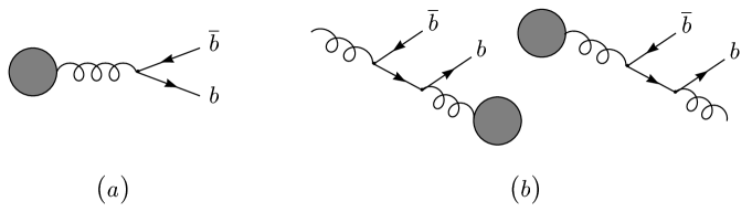
FIG. 7.: QCD radiative correction fragments, corresponding to (a) $g\to b\bar{b}$ and (b) $g\to b\bar{b}g$ splitting. The shaded blob represents the rest of the Feynman graph. Care has to be taken to count these contributions only once when combining relevant backgrounds.

Since our calculation includes full matrix elements to a high order in perturbation theory, care has to be taken to avoid overlap with other backgrounds and double-counting. Closer inspection of the matrix elements for the $t\bar{t}$ and $t\bar{t}j$ modes yields two groups of Feynman diagrams that are candidates for double-counting. They are schematically depicted in Fig. 7. Consider $gu\to b\bar{b}W^{+}W^{-}u$, a subprocess of $t\bar{t}j$ production, as an example. Graph (a) represents $g\to b\bar{b}$ splitting for a final state gluon. It constitutes a QCD radiative correction to $gu\to W^{+}W^{-}ug$ and should be counted in the QCD $WWjj$ background. For small $b\bar{b}$ invariant masses, graph (a) is a contribution to the gluon fragmentation, which must be counted only once. Group (b) features $g\to b\bar{b}g$ splitting, where the $b$-quarks and one gluon are external particles. When the on-shell gluon is in the initial state and the $\bar{b}$ is collinear to it, this group represents an $\alpha_{s}$ correction to $bu\to uW^{+}W^{-}b$ production. When both the $b$ and the $\bar{b}$ are collinear to the initial gluon, we are considering an $\alpha_{s}^{2}$ QCD correction to $gu\to uW^{+}W^{-}$. It is inappropriate to include either group as non-resonant contributions to $t\bar{t}j$ production. These splitting contributions can be eliminated either through suitable cuts or by explicitly excluding the relevant Feynman graphs. A numerical comparison shows that typical selection cuts, like for the Higgs search to be considered in Section IV, are sufficient to render the splitting contributions negligible. Since the analyses in Refs. [8] and [10] do not include QCD corrections to general $WWjj$ production, we chose to omit these graphs in our final calculations. This is permissible since the graphs of group (a) and (b) necessarily contain electroweak interactions of $u$ and $d$ quarks. In the context of top backgrounds, the primary focus is on electroweak interactions of bottom and top quarks. When CKM mixing is neglected, the gauge invariance of our amplitudes is preserved when setting all electroweak interactions of the first two quark generations to zero. This procedure eliminates the graphs of groups (a) and (b) and avoids double-counting.

When integrating over collinear $g\to b\bar{b}$ configurations for initial state gluons, the differential cross section receives enhancement factors of order $\log(\mu_{f}^{2}/m_{b}^{2})$. Since $\alpha_{s}(m_{t})\log(m_{t}^{2}/m_{b}^{2})\approx 0.85$, one may wonder whether our perturbative leading-order calculations are still reliable, or whether a resummation of these collinear logarithms is required. The correct treatment of the collinear region would include $gb$ scattering, convoluted with the $b$-quark parton density. Then, a subtraction of the gluon splitting term would also be required to avoid double-counting [11, 12].

In the cases at hand, the net effect of the $b$-quark PDF contribution is small, however. For inclusive $pp\to b\bar{b}WW,$ only 10.4 pb are added to 622 pb (see Table 1 in Ref. [13]) . For the SM Higgs searches via weak boson fusion, discussed in Section IV, the tagging criteria and selection cuts are chosen such that for $t\bar{t}$ production both $b$-quarks are resolved, with $p_{T}>20$ GeV. This avoids the collinear region. For $t\bar{t}$+1 jet production, the $b$-quark observed as a forward tagging jet is required to have $p_{T}>20$ GeV, while the other $b$-quark has no lower transverse momentum threshold. However, these collinear regions contribute little to the cross section within typical cuts. For example, in the $H\to\tau\tau\to e^{\pm}\mu^{\mp}p\hskip-5.03125pt\hbox to5.03125pt{\hss$/$\hss}_{T}$ search with forward jet tagging cuts [10], the phase space region with $p_{T}<20$ GeV for the untagged $b$- (or $\bar{b}$-) quark contributes only 8% to the total cross section.

The smallness of these collinear effects is related to the fact that we are generating jets and $b$-quarks of $p_{T}>20$ GeV as explicit partons in our calculations. In order to avoid double counting, the factorization scale in the $b$-quark PDF should then be chosen as $\mu_{f}=20$ GeV, which mitigates the role of the collinear logarithms, $\alpha_{s}\log(\mu_{f}^{2}/m_{b}^{2})$. We conclude that a special treatment of collinear effects is not required in our studies. We regularize the $b$-quark collinear region by the finite $b$-quark mass, which provides a simplified but adequate model for the $b$-quark PDF.

Differential cross sections for top production in the narrow-width approximation are independent of $m_{H}$. However, once all off-shell effects are included, a dependence on $m_{H}$ is caused by Higgs propagators that appear in the non-resonant contributions of Fig. 5(f). This dependence has a negligible effect on the rates considered in this paper.

B Phase Space Generator for $t\bar{t}j$ Production and Numerical Tests

FIG. 8.: Phase space decomposition for $bbWW$ final state based on the variables $n_{t}=(m_{bW^{+}}-m_{t})/\Gamma_{t}$ and $n_{\bar{t}}=(m_{\bar{b}W^{-}}-m_{t})/\Gamma_{t}$. The calculation presented here employs separate, hand-optimized phase space generators for double- ($D$), single- ($S_{t}$ and $S_{\bar{t}}$) and non-resonant ($N$) phase space regions. By default the boundaries are chosen at $|n_{t,\bar{t}}|=8$.

While a simple phase space generator proved sufficient for $t\bar{t}$ production, for $t\bar{t}j$ production with significant selection cuts a composite phase space generator that interfaces optimized mappings for double-, single- and non-resonant phase space regions becomes a necessity. These three regions are defined with the help of the two variables

$$n_{t}=\frac{m_{bW^{+}}-m_{t}}{\Gamma_{t}}\qquad\mbox{and}\qquad n_{\bar{t}}=\frac{m_{\bar{b}W^{-}}-m_{t}}{\Gamma_{t}}$$ (18)

The double-resonant region is then defined by $|n_{t}|,|n_{\bar{t}}|<n_{c}$, the single-resonant region by $(|n_{t}|<n_{c}\wedge|n_{\bar{t}}|>n_{c})\vee(|n_{t}|>n_{c}\wedge|n_{\bar{t}}|<n_{c})$ and the non-resonant region by $|n_{t}|,|n_{\bar{t}}|>n_{c}$ (see Fig. 8). In our calculations the boundary parameter $n_{c}$ is chosen to be 8 by default (but see tests below). Since the runtime of the $t\bar{t}j$ program is fairly long, the code currently evaluates only the $S_{t}$ region and multiplies the result by two to account for $S_{\bar{t}}$. This symmetry assumption can easily be removed in the source code should the need arise.

To assure the correctness of the programs three tests were performed. First, the Lorentz-invariance of the modified matrix elements is highly sensitive to errors. A suitable test variable can be defined in the following way: One generates a phase space configuration and evaluates the matrix element squared, summed over all helicity combinations. Applying an arbitrary boost (with $\gamma<5$) to all external momenta and re-evaluating the matrix element, one finally computes

$$\left|1-\frac{\sum|{\cal M}_{\scriptstyle boosted}|^{2}}{\sum|{\cal M}|^{2}}\right|\;.$$ (19)

Evaluating $50\!\cdot\!10^{6}$ phase space configurations (within the forward jet tagging cuts of Ref. [10]), we found an average (maximal) test variable of $2\!\cdot\!10^{-10}$ ($7\!\cdot\!10^{-8}$) for $t\bar{t}$ and $1\!\cdot\!10^{-10}$ ($2\!\cdot\!10^{-5}$) for $t\bar{t}j$.
The test variable is highly sensitive to errors in the matrix element: Omitting the overall factors for a single amplitude that corresponds to a single-resonant Feynman diagram, increases the average and maximal test variable by 5-6 orders of magnitude. Second, the same test variable was used to check the modifications that are necessary to implement the reduction in Fig. 6.

A more recent MADGRAPH version can be used (with minor modifications) to automatically generate the full matrix elements of Eqs. (9) and (10) with 8 and 9 external particles, respectively. These matrix elements can then be compared numerically to the factorized matrix elements in our programs. All overall factors need to be set to 1 for this test and finite widths for space-like top propagators need to be restored. A single, wrong coupling constant, e.g. $g_{Zu}$ rather than $g_{Zd}$, increases the average and maximal test values by 11-13 orders of magnitude.

Finally, the phase space generation for $t\bar{t}$ has been tested by comparing with known cross sections for the Tevatron and the LHC. The composite phase space generation for $t\bar{t}j$ has been checked by moving the boundary between phase space regions, i.e. changing the value of $n_{c}$. For different cut sets and $n_{c}=$ 4, 8 and 16 top-widths, we obtained results consistent within statistical errors of less than 1%. For $t\bar{t}j$ one can explicitly take the narrow top-width limit and compare with the results in Ref. [8], for example. The programs passed all tests.

In order to achieve an accuracy of 1% in a practical time, the programs use an enhanced version of the VEGAS algorithm [27, 28]. It applies importance sampling also to the summation of physical helicity combinations and separately optimizes suitably chosen combinations of subprocesses/phase space regions.

C Numerical Results

First numerical results were obtained using CTEQ4L parton distribution functions as a default, with $\alpha_{s}(m_{Z})=0.132$[29]. The renormalization and factorization scales $\mu_{\scriptstyle r,f}$ are fixed to the top mass, $m_{t}=175$ GeV. In contrast to the Tevatron, top production at the LHC is dominated by the gluon-gluon channel and hence noticeably affected by uncertainties of the gluon density. To assess the impact of effects related to PDF and $\alpha_{s}(m_{Z})$ choice, we compared CTEQ4L and CTEQ5L parton distribution functions [30]. Studying the basic process $pp\to t\bar{t}$, one obtains 622 and 510 pb for CTEQ4L and $\alpha_{s}(m_{Z})=0.132$ and 0.118, respectively. On the other hand, for CTEQ5L and $\alpha_{s}(m_{Z})=0.127$ and 0.118 one gets 560 and 487 pb, respectively, suggesting an overall uncertainty of about 10 or 20% related to the choice of PDF and $\alpha_{s}(m_{Z})$ related to it. With selection cuts, we found similar deviations. For example, in Table VI below, switching from CTEQ4L to CTEQ5L leads to a 4-8% decrease in cross sections at the forward tagging cuts level.

TABLE II.: Comparison of inclusive cross sections with and without finite top width effects. All results are given in pb. The first four columns represent our results: full $t\bar{t}$ cross section including off shell effects, contribution within $|m_{bW^{+}}-m_{t}|>n_{c}\Gamma_{t}$ or $|m_{\bar{b}W^{-}}-m_{t}|>n_{c}\Gamma_{t}$ with $n_{c}=$ 10 and 15, difference to the NWA result, and this difference as a fraction of the total. The $Wt$ column uses results from Table 1 in Ref. [13] for $pp\to b\bar{b}WW$ and Table 1 in Ref. [6] for $pp\to b\bar{b}\ell\bar{\nu}\bar{\ell}\nu$. The results in the second row include leptonic $\tau$ decays, but not $b$ decays. In Ref. [13] different methods are used for $Wt$ to reduce overlap with $t\bar{t}$: $\ \ {}^{\ast)}\ |m_{bW}-m_{t}|>10\Gamma_{t}\ {\rm cut}\quad^{\S)}\ |m_{bW}-m_{t}|>15\Gamma_{t}$ cut.

process	full ${\cal O}(\alpha_{s}^{2}\alpha^{2,4})$	$|m_{bW}-m_{t}|>10/15\Gamma_{t}$	full - NWA	rel.contr.	$W^{-}t+W^{+}\bar{t}$	rel.contr.
$pp\to b\bar{b}WW$	622	63.9/49.6	25	$+4\%$	$66.4^{\ast}/51.6^{\S}$	$+11.1/8.6\%$
$pp\to b\bar{b}\ell\bar{\nu}\bar{\ell}\nu$	39.2	4.0/3.1	1.4	+4%	4.0	+10%

A first comparison of our full calculation with single top production cross sections in the literature is presented in Table II. The two rows correspond to $b\bar{b}WW$ and $b\bar{b}\ell^{+}\nu\ell^{-}\bar{\nu}$ final states, i.e. in the second row off-shell-$W$ corrections are included in our calculation. In our simulation, $b\bar{b}e^{+}\nu\mu^{-}\bar{\nu}$ results were multiplied by a factor 5.48 to account for all lepton flavor combinations, including leptonic $\tau^{\pm}$ decays. Off-shell contributions from $W^{-}t+W^{+}\bar{t}$ final states were calculated in Ref. [13] with several definitions of the off-shell region. These results agree with ours at the 4% level (see second column). The agreement improves to the 1–2% level once double counting effects in the non-resonant regions ($N$-regions of Fig. 8) are taken into account. Compared to this $W^{-}t+W^{+}\bar{t}$ cross section, however, the actual enhancement of the $t\bar{t}$ cross section due to off-shell contributions, calculated as the difference of our full result minus the cross section in the NWA (see column three), is only about half as large.

The problem can be traced to the fact that a Breit-Wigner distribution has long tails, more precisely

$$\int_{(m-n\Gamma)^{2}}^{(m+n\Gamma)^{2}}\frac{1}{(q^{2}-m^{2})^{2}+(m\Gamma)^{2}}\cdot\frac{dq^{2}}{2\pi}\approx\frac{1}{2m\Gamma}\cdot\left(1-\frac{1}{n\pi}\right)\,$$ (20)

i.e. for each of the two top-quark resonances, about 2% of the cross section is located outside an $n=15$ top-widths window, for example. This 4% resonant contribution, which is double-counted when combining the rate in the $|m_{bW}-m_{t}|>15\Gamma_{t}$ region with the $t\bar{t}$ cross section in the narrow width approximation, accounts for the difference between our “full minus NWA” result and the estimate in terms of the $W^{-}t+W^{+}\bar{t}$ cross section. This means that off-shell $t\bar{t}$ calculations which directly take $W^{-}t+W^{+}\bar{t}$ cross sections as the off-shell rate, tend to produce a serious overestimate of the number of extra events.

Our method of choice to include finite-width effects involves overall factors that are expected to be small in non-resonant regions as explained in Section II. In order to test this expectation in a realistic context, we compared the differential cross section obtained with overall factors with various proxies in different phase space regions (see Fig. 8). In the non-resonant region $N$ the proxy is the tree-level matrix element with unmodified tree-level top quark propagators, because they are not singular and a good approximation to the full propagator in this region. In the single-resonant regions $S_{t}$ and $S_{\bar{t}}$ the proxy is derived from the proxy used in region $N$ by replacing the potentially singular top (in $S_{t}$) or anti-top (in $S_{\bar{t}}$) propagators with fixed-width propagators, i.e.

$$\frac{i(p\hskip-5.03125pt\hbox to5.03125pt{\hss$/$\hss}+m_{t})}{p^{2}-m_{t}^{2}+im_{t}\Gamma_{t}}\quad.$$ (21)

FIG. 9.: Integrated transverse momentum distribution for the additional massless parton (jet) in off-shell $t\bar{t}j$ production: $\sigma(p_{Tj}^{\text{min}})=\int_{p_{Tj}^{\text{min}}}^{\infty}(d\sigma/dp_{Tj})\,dp_{Tj}$. No selection cuts are applied. For $p_{Tj}^{\rm min}=40$ GeV one obtains $\sigma_{t\bar{t}j}\approx\sigma_{t\bar{t}}=39.2$ pb (dotted line, see Table II).

In the double-resonant region $D$ the proxy matrix element is a subset of all Feynman diagrams, namely all diagrams with at least one time-like top propagator. Since all these top propagators are potentially resonant here, they all feature the fixed-width form of Eq. (21). Each region is covered by 20-28 bins. Bin sizes are adjusted so that each value roughly has the same integration error. For each bin the relative deviation from the proxy is estimated by

$$\left|\int_{\scriptstyle\rm bin}d\sigma_{\scriptstyle\rm fac}-\int_{\scriptstyle\rm bin}d\sigma_{\scriptstyle\rm proxy}\right|\;\left/\;\int_{\scriptstyle\rm bin}d\sigma_{\scriptstyle\rm proxy}\right.\quad.$$ (22)

We studied this measure for $t\bar{t}$ production without cuts as well as the forward tagging cuts of Refs. [8] and [10] and found similar results. In the double- and single-resonant regions the overall factor scheme deviates from the proxies by 2% or less, and the deviation drops to less than 1% in the non-resonant region. We therefore estimate the error associated with our finite-width scheme to be of ${\cal O}$(1%), which is comparable to the statistical error of our results, but completely negligible compared to missing higher order QCD corrections. These results suggest that our method to include finite-width effects provides reliable results, not only for fairly inclusive cross sections, where finite width effects are strongly suppressed, but also when complex selection cuts result in on- and off-shell contributions of similar size.

Comparing inclusive cross sections, we find $B\sigma_{t\bar{t}}=39.2$ pb in Table II. Including an additional jet we obtain $B\sigma_{t\bar{t}j}=80$ pb, when a common $p_{T}>20$ GeV cut is imposed on the additional jet. This raises the question, whether the cut should typically be chosen higher, such that $\sigma_{t\bar{t}j}\lesssim\sigma_{t\bar{t}}$, i.e. $\sigma_{t\bar{t}j}$ is sub-dominant, as typically expected for a NLO QCD correction. The integrated $p_{Tj}$ distribution of the non-$b$ parton is shown in Fig. 9. For $p_{Tj}^{\rm min}=40$ GeV one obtains $\sigma_{t\bar{t}j}\approx\sigma_{t\bar{t}}$. Real parton emission cross sections saturating the LO cross section at low $p_{T}$ of the extra parton are a sign of copious multi-jet production in actual data [31].

The additional parton emission is dominated by initial state radiation. This can be inferred from the invariant mass distributions of the potential top-quark decay products, the $bW^{+}$ and the $bW^{+}j$ systems shown in Fig. 10. The $m_{bW^{+}}$ invariant mass distribution in Fig. 10(a) contains 85% of the total cross section in the displayed 165-185 GeV window around the top resonance ($\pm 6.4\Gamma_{t}$). In contrast, the same $m_{bW^{+}j}$ invariant mass window (insert of Fig. 10(b)) accounts for only 10% of the total cross section. Final state radiation is relatively unimportant in $t\bar{t}j$ production at the LHC.

FIG. 10.: Invariant mass distribution of potential top-quark decay products (a) $bW^{+}$ and (b) $bW^{+}j$ in $t\bar{t}j$ production, including full finite width effects. No selection cuts are applied, except for a $p_{Tj}>20$ GeV cut on the final state massless parton. Cross sections correspond to one lepton-flavor combination only.

IV Application to SM Higgs search at the LHC

TABLE III.: Numbers of expected $pp\to b\bar{b}\ell\bar{\nu}\bar{\ell}\nu$ background events in the ATLAS $H\to WW^{*}$ Higgs search for an integrated luminosity of 30 fb^-1. Basic ATLAS TDR background suppression cuts are applied [5, 6]. ATLAS detector effects are simulated as described in Section II.F in Ref. [8]. The left columns show our results for the four $W\to e\nu,\mu\nu$ lepton combinations. The right columns are the corresponding results from Table 2 in Ref. [6]. For both categories, the relative change due to the inclusion of finite width effects is given as an enhancement factor in the third column.

$m_{T}$ window [GeV]	top in NWA	full off-shell	rel. chg.	$t\bar{t}$	$t\bar{t}+Wt$	rel. chg.
120–150	50	93	1.9	41	206	5.0
130–160	50	96	1.9	66	204	3.1
140–170	43	83	1.9	51	146	2.9
140–180	49	95	1.9	61	164	2.7
150–190	35	68	1.9	56	111	2.0

An important application of $t\bar{t}{j}$ production as a background occurs in Higgs physics. Higgs mass limits have recently been pushed to $m_{H}>114.1$ GeV by the LEP experiments [32]. As a result, the LHC search for $H\to WW$ [3, 4, 5, 6, 7, 8] and $H\to\tau\tau$ [5, 9, 10] decays in the intermediate mass range has gained even greater importance. For the $H\to WW\to\ell^{\pm}\ell^{\mp}p\hskip-5.03125pt\hbox to5.03125pt{\hss$/$\hss}_{T}$ decay mode, top-quark decays constitute the largest reducible background. The impact of this background has been analyzed, in the narrow-width approximation, for Higgs masses around 170 GeV [5, 6, 8] and most recently for a light Higgs boson with $m_{H}\approx 115$ GeV [7]. This background also plays a role in the $H\to\tau\tau\to e^{\pm}\mu^{\mp}p\hskip-5.03125pt\hbox to5.03125pt{\hss$/$\hss}_{T}$ decay mode, which was analyzed in the narrow-width approximation in Ref. [10]. In this section we present updated results for these analyses obtained with our parton-level Monte Carlo program that includes off-shell top and $W$ effects and takes into account the single-resonant and non-resonant contributions.

A $t\bar{t}$ Backgrounds to Inclusive $H\to WW$ Searches

The $t\bar{t}$ background calculations (without an additional jet) are most relevant for inclusive $H\to WW$ searches [3, 4, 5], where Higgs production is dominated by the gluon fusion process. In Tables III and IV we compare the relative contributions from off resonant top effects for two selections of $H\to WW\to\ell^{\pm}\ell^{\mp}p\hskip-5.03125pt\hbox to5.03125pt{\hss$/$\hss}_{T}$ events in ATLAS, as described in Refs. [5, 6]. The selection looks for two isolated, opposite charge leptons of $p_{T}>20,10$ GeV within the pseudo-rapidity range $|\eta_{\ell}|<2.5$ and of invariant mass $m_{\ell\ell}<80$ GeV. Events must have significant missing $E_{T}$, $E\hskip-7.95831pt\hbox to7.95831pt{\hss$/$\hss}_{T}>40$ GeV. A small angle between the charged leptons favors $H\to WW$ decays versus backgrounds. Finally, a veto on additional jets in the central region is very effective against the $b$-quark jets in the top-quark backgrounds. The main difference between Tables III and IV is the definition of this veto on jet activity with $p_{T}>15$ GeV in the central region. It is imposed within $|\eta_{j}|<3.2$ in Table III and within $|\eta_{j}|<2.4$ in Table IV.

FIG. 11.: Transverse mass distribution for the low-luminosity ATLAS selection cuts of Ref. [5], Section 19.2.6, and Ref. [6]. The dotted curve shows the distribution obtained when treating the top quarks in the narrow-width approximation while the solid curve includes all off-shell effects.

In addition, the selection looks for events inside the Jacobian peak of the dilepton-$E\hskip-7.95831pt\hbox to7.95831pt{\hss$/$\hss}_{T}$ transverse mass distribution, as indicated in the first column of the two tables. Here the transverse mass is defined as

$$m_{T}(\ell\ell,E\hskip-7.95831pt\hbox to7.95831pt{\hss$/$\hss}_{T})=\sqrt{2p_{T}^{\ell\ell}E\hskip-7.95831pt\hbox to7.95831pt{\hss$/$\hss}_{T}[1-\cos\Delta\theta(\ell\ell,E\hskip-7.95831pt\hbox to7.95831pt{\hss$/$\hss}_{T})]}\;.$$ (23)

Fig. 11 shows this transverse mass distribution underlying the ATLAS TDR analysis. Off-shell contributions raise the normalization of the $t\bar{t}$ background by about a factor of 2, but have little effect on the shape of the background, for $m_{T}\gtrsim 120$ GeV. The ATLAS analysis attempts to take (single-resonant) off-shell effects into account via on-shell $Wt$ calculations. As the comparison in Table III shows, our unified calculation indicates a lower background increase than the combined on-shell $t\bar{t}$ and $Wt$ calculations would suggest. This observation is consistent with the small increase due to off-resonant effects observed in Table II.

For a precise comparison with the ATLAS simulation, the nature of the programs (parton-level MC with full matrix elements vs. event generator with parton showers/hadronization) is currently too different. In particular our program does not allow to simulate the effect of the central jet veto on extra gluon radiation in the event. Also, we did not include any detector efficiencies. We would expect an extra suppression, by perhaps a factor of 3 to 4, of the “full off-shell” results in Tables III and IV due to these effects, i.e. the apparent agreement of the $t\bar{t}$ cross section with our NWA result in Table III is somewhat fortuitous. This suspicion is confirmed by the fairly large disagreement between our NWA or full off-shell results and the PYTHIA simulation in Table IV.

TABLE IV.: Same as Table III, but for the optimized background suppression cuts of Ref. [6].

$m_{T}$ window [GeV]	top in NWA	full off-shell	rel. chg.	$t\bar{t}$	$t\bar{t}+Wt$	rel. chg.
120–150	364	536	1.5	107	346	3.2
130–160	363	544	1.5	122	306	2.5
140–170	310	465	1.5	82	215	2.6
140–180	352	528	1.5	107	254	2.4
150–190	251	374	1.5	87	168	1.9

At present the source of these discrepancies is not completely understood. The rapidity distribution of $b$-quarks in our full matrix element calculation appears to be wider than in the PYTHIA generated events, potentially due to approximations in the top decay chain in PYTHIA. This makes a veto over a smaller pseudo-rapidity range less efficient. On the other hand we cannot simulate the effect of additional gluon radiation. A reanalysis of these effects, combining full matrix elements with a parton shower Monte Carlo, including hadronization, is clearly warranted, given that top-quark production constitutes about half the background to the inclusive $H\to WW$ search[6].

While the overall background normalization requires further study, the ratio of “full off-shell” and NWA results is expected to be robust, i.e. it will be little affected by detector efficiencies and by higher order gluon radiation. These ratios are given in the third columns, marked “relative change”, in Tables III and IV. Our results clearly indicate that the increase in top-backgrounds due to the inclusion of off-shell effects (the $Wt$ contribution in the ATLAS analysis) is substantially smaller than previously thought.

In a LO calculation, substantial uncertainties arise from ambiguities in the choice of factorization and renormalization scales. For the double resonant phase space configurations, $\mu_{\scriptstyle r}=\mu_{\scriptstyle f}=m_{t}$ or the transverse energy of the top quarks are well-motivated choices. When forcing the $b$-quarks to low $p_{T}$ values by a central jet veto and simultaneously enhancing the off-shell phase space regions, a smaller renormalization and/or factorization scale may be more appropriate. The impact of a lower scale on the full off-shell results in Table III is demonstrated by the scale choice

$$\mu_{\scriptstyle r,f}=\left\{\begin{array}[]{r@{\quad\mbox{if}\quad}l}m_{t}&|m_{bW^{+}}-m_{t}|<4\Gamma_{t}\;\,\wedge\;\,|m_{\bar{b}W^{-}}-m_{t}|<4\Gamma_{t}\\ 20\ \mbox{GeV}&|m_{bW^{+}}-m_{t}|>4\Gamma_{t}\;\,\vee\;\,|m_{\bar{b}W^{-}}-m_{t}|>4\Gamma_{t}\end{array}\right.$$ (24)

where the value of 20 GeV is motivated by the veto threshold for central jets. Resulting cross sections are about 65% higher than the rates obtained with $m_{t}$ as a universal scale. A NLO calculation would be needed to distinguish the virtue of either choice. At present, this variation indicates the uncertainty of our LO results.

B $t\bar{t}(j)$ Backgrounds in Weak Boson Fusion Studies

In addition to the inclusive search for $H\to WW$ events, weak boson fusion (WBF) presents a very attractive search channel for $H\to WW$ and $H\to\tau\tau$ events and will likely play a crucial role in the measurement of Higgs boson couplings to fermions and gauge bosons [33]. Top quark decays again form an important background in these searches and, due to the central jet veto proposed for the reduction of QCD backgrounds, off-shell effects might be important. The signal and backgrounds for $H\to WW\to e^{\pm}\mu^{\mp}p\hskip-5.03125pt\hbox to5.03125pt{\hss$/$\hss}_{T}$ and $H\to\tau\tau\to e^{\pm}\mu^{\mp}p\hskip-5.03125pt\hbox to5.03125pt{\hss$/$\hss}_{T}$ in WBF were analyzed in Refs. [8] and [10], respectively, with the top-quark backgrounds determined in the NWA, however. With our new programs we are able to update these background estimates, including off-shell contributions.

Because of the two additional jets which are present in the WBF process $qq\to qqH$, the dominant top quark background arises from $t\bar{t}j$ events. Event selection for WBF requires two tagging jets, of $p_{T}>20$ GeV, which are widely separated in pseudo-rapidity ($|\eta_{1}-\eta_{2}|>4.2$) and which have a very large dijet invariant mass, $M_{jj}>650$ GeV. By definition, the $t\bar{t}$ background has both $b$-quarks identified as tagging jets while in the $t\bar{t}j$ background exactly one $b$ or $\bar{b}$ is taken as a tagging jet. The two $b$-quarks rarely have a large enough dijet mass or are far enough separated to satisfy the tagging criteria, and this leaves $t\bar{t}j$ events as the dominant background to WBF. This result holds in both the NWA and with inclusion of off-resonant effects as is evident in both Tables V and VI, at all cut levels.

The veto of central jets of $p_{T}>20$ GeV is effective against the extra $b$-quark jet and off-shell contributions are only slightly enhanced after this cut (see line “$b$ veto” in the Tables). Overall, off-shell contributions are fairly modest, increasing the NWA results by about 20% (see the second last columns in the Tables). This means that our new complete calculation of off-shell effects in $t\bar{t}j$ production confirms the conclusions about the observability of $H\to\tau\tau$ and $H\to WW$ events reached in Refs. [8] and [10]. Tables V and VI display our updated results. Precise definitions of cuts are given in the earlier papers. A breakdown into subprocesses and phase space regions of the overall $t\bar{t}j$ background of 351 fb to $H\to WW\to e^{\pm}\mu^{\mp}p\hskip-5.03125pt\hbox to5.03125pt{\hss$/$\hss}_{T}$, after forward jet tagging cuts, is given in Table VII.

TABLE V.: $t\bar{t}(j)$ background cross sections for $H\to WW\to e^{\pm}\mu^{\mp}p\hskip-5.03125pt\hbox to5.03125pt{\hss$/$\hss}_{T}$ for $m_{H}=160$ GeV in $pp$ collisions at $\sqrt{s}=14$ TeV. Results are given for various levels of cuts and are labeled by equation numbers from Ref. [8]. All cross sections are given in fb. Cuts and other calculational details are described in Ref. [8]. The integration error is 1% or better. The signal over background ratio is also shown. Cross sections not listed here are as in Table I in Ref. [8].

	top in NWA			full off-shell
cuts	$t\bar{t}$	$t\bar{t}j$	S/B	$t\bar{t}$		$t\bar{t}j$		S/B
forward tagging (10)-(12)	12.4	308	$\approx$1/65	13.0	+4.4%	351	+14%	$\approx$1/67
+ $b$ veto (13)		43.5	1/5.1			51.4	+18%	1/5.6
+ $M_{jj}$, angular cuts (14)-(16)	0.0551	4.67	1.1/1	0.0761	+38%	5.42	+16%	1.0/1
+ real $\tau$ rejection (17)	0.0527	4.34	1.7/1	0.0737	+40%	5.09	+17%	1.5/1
$P_{surv,20}$ (${\it\times 0.29}$) + (18)	0.0153	1.26	4.6/1	0.0214	+40%	1.48	+17%	4.2/1
+ tag ID efficiency (${\it\times 0.74}$)	0.0113	0.932	4.6/1	0.0158	+40%	1.09	+17%	4.2/1

TABLE VI.: $t\bar{t}(j)$ background cross sections for $H\to\tau\tau\to e^{\pm}\mu^{\mp}p\hskip-5.03125pt\hbox to5.03125pt{\hss$/$\hss}_{T}$ for $M_{H}=120$ GeV in $pp$ collisions at $\sqrt{s}=14$ TeV. Results are given for various levels of cuts and are labeled by equation numbers from Ref. [10]. All cross sections are given in fb. Cuts and other calculational details are described in Ref. [10]. The integration error is 1% or better. The signal over background ratio is also shown. Cross sections not listed here are as in Table I in Ref. [10].

	top in NWA			full off-shell
cuts	$t\bar{t}$	$t\bar{t}j$	S/B	$t\bar{t}$		$t\bar{t}j$		S/B
forward tagging (7)-(10)	13.5	357	1/1100	15.9	+17%	436	+22%	1/1100
+ $b$ veto (11)		50.1	1/550			63.6	+27%	1/550
+ $p\hskip-5.03125pt\hbox to5.03125pt{\hss$/$\hss}_{T}$ (12)	11.1	43.0	1/74	13.2	+19%	55.2	+28%	1/83
+ $M_{jj}$ (13)	0.593	12.9	1/32	0.712	+20%	15.8	+22%	1/34
+ non-$\tau$ reject. (14, 15, 17)	0.00303	0.257	1/5.8	0.00365	+20%	0.293	+14%	1/5.8

TABLE VII.: Distribution of the $t\bar{t}j$ background to $H\to WW\to e^{\pm}\mu^{\mp}p\hskip-5.03125pt\hbox to5.03125pt{\hss$/$\hss}_{T}$, with forward tagging cuts, among subprocesses (labeled by initial partons) and phase space regions (see Fig. 8). The cut between double resonant ($D$), single resonant ($S_{t}+S_{\bar{t}}$), and non-resonant regions ($N$) is set at 8 top quark widths. Cross sections are given in fb.

	$D$	$S_{t}+S_{\bar{t}}$	$N$
$gg$	171	28.6	1.1
$gq+qg$	128	18.8	0.64
$qq$	2.92	0.35	0.009

V Summary

Top-quarks are a very important source of lepton backgrounds to new physics searches at the LHC: the large production cross section typical for a strong interaction process combines with a sizable branching fraction into leptons which, due to the large mass of the $W$, often survive isolation cuts. Suppression techniques for top quark backgrounds, like a veto on central jets, which is very effective against the $b$-quarks of the $t\to bW\to b\ell\nu$ decay chain, enhance the relative importance of off-resonant effects and may exacerbate errors introduced by approximate modeling of matrix elements. Severe cuts select the tails of various distributions and these phase space regions may well differ from the ones for which the models were optimized originally. General purpose Monte Carlo programs like PYTHIA[34] or Herwig[35] should thus be gauged against matrix element programs.

In this paper we have presented results for two new programs which allow to model the $t\bar{t}\to b\bar{b}WW\to b\bar{b}\ell^{+}\nu\ell^{-}\bar{\nu}$ decay chain at tree level, including full angular correlations of all top and $W$ decay products and with proper interpolation between double-resonant, single-resonant and non-resonant phase space regions. These full correlations are available for $t\bar{t}$ and $t\bar{t}j$ production. Electroweak and $SU(3)$ gauge invariance is maintained throughout, by employing the overall factor scheme for the Breit Wigner propagators of all unstable particles in the $t$ and $\bar{t}$ decay chains.

Comparing to earlier calculations of off-shell effects, via the $gb\to Wtb$ production cross sections, we find excellent agreement when avoiding the top-quark resonance for the $Wb$ system. However, some earlier combinations of $t\bar{t}$ and $Wtb$ cross sections have involved substantial double counting, leading to an overestimate of backgrounds in e.g. Higgs search analyses at the LHC. In addition, the full simulation of $V-A$ couplings in the $t\to Wb\to\ell\nu b$ decay chain is available with our programs and may have sizable effects in background estimates.

When considering $t\bar{t}$ backgrounds to Higgs searches, off-shell effects are most pronounced in inclusive $H\to WW$ analyses, where both $b$-quark jets may be vetoed. In weak boson fusion studies the additional jets in the signal selection make the background suppression due to the jet veto less severe, which diminishes the overall importance of off-shell contributions.

Our programs now allow detailed study of these off-shell effects in top pair backgrounds with zero or one additional parton in the final state.

- [1] F. Abe et al. [CDF Collaboration], Phys. Rev. Lett. 74, 2626 (1995); S. Abachi et al. [D0 Collaboration], Phys. Rev. Lett. 74, 2632 (1995).
- [2] S. Abel et al., SUGRA Working Group Report, (2000) [hep-ph/0003154]; H. Baer, J. K. Mizukoshi, and X. Tata, Phys. Lett. B488, 367 (2000); H. Baer, P. G. Mercadante, X. Tata, and Y. Wang, Phys. Rev. D62, 095007 (2000); V. Barger and C. Kao, Phys. Rev. D60, 115015 (1999); K. T. Matchev and D. M. Pierce, Phys. Rev. D60, 075004 (1999); H. Baer et al., Phys. Rev. D61, 095007 (2000); W. Beenakker et al., Phys. Rev. Lett. 83, 3780 (1999); H. E. Haber and G. L. Kane, Phys. Rept. 117, 75 (1985).
- [3] M. Dittmar and H. Dreiner, Phys. Rev. D55, 167 (1997); and [hep-ph/9703401].
- [4] G. L. Bayatian et al., CMS Technical Proposal, report CERN-LHCC-94-38, (1994); R. Kinnunen and D. Denegri, CMS NOTE 1997/057, (1997); R. Kinnunen and A. Nikitenko, CMS TN/97-106, (1997); R. Kinnunen and D. Denegri, CMS NOTE 1999/037, (1999).
- [5] ATLAS Collaboration, report CERN-LHCC-99-15, (1999).
- [6] K. Jakobs and T. Trefzger, note ATL-PHYS-2000-015, (2000).
- [7] N. Kauer, T. Plehn, D. Rainwater, and D. Zeppenfeld, Phys. Lett. B503, 113 (2001).
- [8] D. Rainwater and D. Zeppenfeld, Phys. Rev. D60, 113004 (1999).
- [9] D. Rainwater, D. Zeppenfeld, and K. Hagiwara, Phys. Rev. D59, 014037 (1999).
- [10] T. Plehn, D. Rainwater, and D. Zeppenfeld, Phys. Rev. D61, 093005 (2000).
- [11] A. S. Belyaev, E. E. Boos, and L. V. Dudko, Phys. Rev. D59, 075001 (1999).
- [12] T. M. P. Tait, Phys. Rev. D61, 034001 (2000).
- [13] A. Belyaev and E. Boos, Phys. Rev. D63, 034012 (2001).
- [14] T. Stelzer, Z. Sullivan, and S. Willenbrock, Phys. Rev. D58, 094021 (1998); T. Tait and C. P. Yuan, Phys. Rev. D63, 014018 (2001); M. C. Smith and S. Willenbrock, Phys. Rev. D54, 6696 (1996); S. Mrenna and C. P. Yuan, Phys. Lett. B416, 200 (1998); T. Stelzer, Z. Sullivan, and S. Willenbrock, Phys. Rev. D56, 5919 (1997); T. Tait and C. P. Yuan, Phys. Rev. D55, 7300 (1997).
- [15] T. Stelzer and W. F. Long, Comput. Phys. Commun. 81, 357 (1994).
- [16] H. Murayama, I. Watanabe, and K. Hagiwara, report KEK-91-11, (1992).
- [17] U. Baur and D. Zeppenfeld, Phys. Rev. Lett. 75, 1002 (1995).
- [18] E. N. Argyres et al., Phys. Lett. B358, 339 (1995).
- [19] W. Beenakker et al., Nucl. Phys. B500, 255 (1997).
- [20] N. Kauer, Master’s thesis, University of Wisconsin-Madison, 1996.
- [21] U. Baur et al., Phys. Rev. D56, 140 (1997).
- [22] K. Hagiwara, K. Hikasa, R. D. Peccei, and D.Zeppenfeld, Nucl. Phys. B282, 253 (1987); U. Baur and D. Zeppenfeld, Phys. Lett. 201B, 383 (1988).
- [23] U. Baur, J. Vermaseren, and D. Zeppenfeld, Nucl. Phys. B375, 3 (1992).
- [24] A. Denner, S. Dittmaier, M. Roth, and D. Wackeroth, Nucl. Phys. B560, 33 (1999).
- [25] G. Lopez Castro, J. L. Lucio, and J. Pestieau, Mod. Phys. Lett. A6, 3679 (1991); M. Nowakowski and A. Pilaftsis, Z. Phys. C60, 121 (1993); M. Beuthe, R. Gonzalez Felipe, G. Lopez Castro, and J. Pestieau, Nucl. Phys. B498, 55 (1997); G. Lopez Castro and G. Toledo Sanchez, Phys. Rev. D61, 033007 (2000).
- [26] J. van der Heide, E. Laenen, L. Phaf, and S. Weinzierl, Phys. Rev. D62, 074025 (2000).
- [27] G. P. Lepage, J. Comput. Phys. 27, 192 (1978).
- [28] G. P. Lepage, preprint CLNS-80/447, (1980).
- [29] H. L. Lai et al., Phys. Rev. D55, 1280 (1997).
- [30] H. L. Lai et al., Eur. Phys. J. C12, 375 (2000).
- [31] D. Rainwater, R. Szalapski, and D. Zeppenfeld, Phys. Rev. D54, 6680 (1996).
- [32] ALEPH, DELPHI, L3, and OPAL Collaborations, LHWG NOTE/2001-03, (2001) [hep-ex/0107029].
- [33] D. Zeppenfeld, R. Kinnunen, A. Nikitenko, and E. Richter-Wa̧s, Phys. Rev. D62, 013009 (2000).
- [34] T. Sjostrand et al., Comput. Phys. Commun. 135, 238 (2001).
- [35] G. Corcella et al., JHEP 01, 010 (2001); and [hep-ph/0107071].