CERN-TH/2001–184

hep-ph/0107156 IFUP–TH/18–2001

Phenomenological implications of
neutrinos in extra dimensions

André de Gouvêa, Gian Francesco Giudice,
Alessandro Strumia, and Kazuhiro Tobe

Theoretical Physics Division, CERN, CH-1211, Genève 23, Switzerland

Abstract

Standard Model singlet neutrinos propagating in extra dimensions induce small Dirac neutrino masses. While it seems rather unlikely that their Kaluza-Klein excitations directly participate in the observed neutrino oscillations, their virtual exchange may lead to detectable signatures in future neutrino experiments and in rare charged lepton processes. We show how these effects can be described by specific dimension-six effective operators and discuss their experimental signals.

1 Introduction

The hypothesis that Standard Model (SM) singlet fields propagate in extra dimensions leads to striking results. When applied to the graviton, it allows to lower the quantum gravity scale down to few TeV [1, 2], suggesting a new scenario for addressing the Higgs mass hierarchy problem. It is also natural to consider the case of “right-handed neutrinos” (i.e., fermions without SM gauge interactions) propagating in extra dimensions. The smallness of the neutrino masses, of the Dirac type, could in fact be a manifestation of this hypothesis [3, 4, 5, 6].

If the radius of the compactified dimensions is very large, $R\,\raise 1.29167pt\hbox{$>$\kern-7.5pt\lower 4.30554pt\hbox{$\sim$}}\,\,{\rm eV}^{-1}$, Kaluza-Klein (KK) modes of right-handed neutrinos would significantly participate in neutrino oscillations. However, KK interpretations of the atmospheric and solar neutrino puzzles are disfavoured by the following arguments:

• A KK tower of sterile neutrinos gives rise to active/sterile oscillations at a small $\Delta m^{2}\sim 1/R^{2}$ only in the case of a single large extra dimension. In the case of more large extra dimensions, the active/sterile mixing is not dominated by the lightest KK modes, and the mixing with the heaviest KK modes does not lead to oscillations. One could argue that right-handed neutrinos in a single very large extra dimension can be effectively obtained if one of the extra dimensions happens to be much larger than the other(s). However, the fact that infrared effects are dominant in this case destabilises the hierarchy [7]: the Newton or Coulomb potential grows with the size $R$ of the largest dimension.

• Even if one forgets about the hierarchy problem, there are severe bounds from supernovæ observations [8]. One needs to prevent resonant neutrino conversion in supernovæ by choosing a small radius $R\,\raise 1.29167pt\hbox{$<$\kern-7.5pt\lower 4.30554pt\hbox{$\sim$}}\,1/\,{\rm MeV}$ or by adding an ad-hoc 5-dimensional mass term $m\,\raise 1.29167pt\hbox{$>$\kern-7.5pt\lower 4.30554pt\hbox{$\sim$}}\,\,{\rm MeV}$ for the right-handed neutrino(s) responsible for “atmospheric” oscillations. The latter still allows to build models for the solar anomaly roughly compatible with supernovæ bounds [9].

• Finally, the recent results from the SuperKamiokande [10, 11] and SNO [12] experiments provide strong indications for $\nu_{\tau}$ appearance in atmospheric oscillations and for $\nu_{\mu},\nu_{\tau}$ appearance in solar oscillations. In both cases, a sterile interpretation is now strongly disfavoured by experiments.

In this paper we explore the phenomenology of more promising models with $\delta>2$ extra dimensions and radii which are not larger than what is required to reproduce the gauge/gravitation hierarchy. The neutrino puzzles are solved by “normal” (active) oscillations, but the presence of the heaviest KK neutrinos can still lead to small but detectable effects in neutrino flavour transitions. After integrating out the heavy KK modes, we obtain an effective Lagrangian that contains massive Dirac neutrino states and a specific set of non-renormalizable operators. Since the dominant effects come from the heaviest KK states, the coefficients of these operators can only be estimated by introducing an arbitrary ultraviolet cut-off.

At tree level one only obtains the dimension-six operators

$${\cal L}_{\rm tree}=\epsilon_{ij}~{}2\sqrt{2}G_{F}(H^{\dagger}\bar{L}_{i})i\partial\!\!\!\raisebox{2.0pt}[0.0pt][0.0pt]{$\scriptstyle/$}(HL_{j}),$$ (1.1)

where $L_{i}$ are the lepton left-handed doublets, $H$ is the Higgs doublet, and $\epsilon_{ij}=\epsilon_{ji}^{*}$ are dimensionless couplings. The presence of these effective operators leads, for example, to potentially large flavour transitions $P(\nu_{i}\to\nu_{j})\sim|\epsilon_{ij}^{2}|$ at ${\cal O}(L^{0})$ (i.e., at very short baselines $L\ll E_{\nu}/\Delta m^{2}$), and CP-violating effects at ${\cal O}(L^{1})$ (rather than at ${\cal O}(L^{2})$ and ${\cal O}(L^{3})$ as in ordinary oscillations). Since this peculiar tree level operator only affects neutrinos, potentially detectable effects, especially at a neutrino factory, are not already excluded by bounds from rare charged leptons processes, like $\tau\to\mu\gamma$, $\mu\to e\gamma$, $\mu\to e\bar{e}e$, etc. We will show, however, that Eq. (1.1) cannot explain the LSND anomaly [13], due to the present constraints from searches for $\mu\rightarrow e\gamma$.

At one-loop level, other operators are generated, giving rise to rare muon and tau processes that violate lepton flavour. Again, the coefficients of these operators are cut-off dependent and can only be estimated. However, in minimal models, their flavour structure is directly related to the physical neutrino mass matrix, giving predictions for rare muon processes in terms of neutrino oscillation parameters. This is in contrast with other cases of physics beyond the SM. In supersymmetry, for instance, the rates for rare muon processes are perturbatively calculable, but their relations with neutrino oscillations parameters are strongly model-dependent and can vary by many orders of magnitude.

Many of the effects studied here have already been considered in previous analyses [14, 15] as due to mixing between ordinary neutrinos and the whole tower of KK states. The equivalent language of effective operators we employ allows the study of different models (e.g. large and warped extra dimensions) in a unified framework, the discrimination of what is really computable from what can only be estimated, and a more transparent identification of all potentially interesting experimental signatures.

The paper is organized as follows. In Sec. 2, we describe the models under consideration. In Sec. 3 we discuss the effects of the tree level operator Eq. (1.1) in neutrino physics. In Sec. 4 we discuss the effects of the operators induced at one-loop in charged lepton processes. In Sec. 5 we summarize our results.

2 Right-handed neutrinos in extra dimensions

We will study models with large flat extra dimensions [1, 3, 4, 5] and models with one warped extra dimension [2, 6].

Large flat extra dimensions

We consider $(4+\delta)$-dimensional massless fermions $\Psi_{i}(x_{\mu},y)$ which, inside their $2^{(4+\delta)/2}$ components (for even $\delta$) or $2^{(3+\delta)/2}$ components (for odd $\delta$), contain the degrees of freedom of the “right-handed neutrinos” $\nu_{Ri}$ ($i=1,2,3$ is the generation index). The fermions $\Psi_{i}$ interact in our brane, through their components $\nu_{Ri}$, with the standard left-handed lepton doublet $L_{i}$ in a way that conserves total lepton number. The relevant part of the action is

$${\cal S}=\int d^{4}\!x~{}d^{\delta}\!y~{}\bar{\Psi}_{i}iD\!\!\!\raisebox{2.0pt}[0.0pt][0.0pt]{$\scriptstyle/$}\,\Psi_{i}+\int d^{4}\!x~{}\left[\bar{L}_{i}i\partial\!\!\!\raisebox{2.0pt}[0.0pt][0.0pt]{$\scriptstyle/$}\,L_{i}-\left(\bar{L}_{i}\lambda_{ij}\nu_{Rj}H^{\dagger}+\hbox{h.c.}\right)\right],$$ (2.1)

where $iD\!\!\!\raisebox{2.0pt}[0.0pt][0.0pt]{$\scriptstyle/$}$ is a $4+\delta$ dimensional Dirac operator, $H$ is the SM Higgs doublet in four dimensions and $\lambda$ is a matrix of Yukawa couplings with dimensions ${\rm(mass)}^{-\delta/2}$. As is manifest from Eq. (2.1), $\lambda$ can be made diagonal without loss of generality at the price of introducing the usual unitary matrix $U$, which describes flavour-changing charged current neutrino interactions.

Using the KK decomposition

$$\Psi_{i}(x,\vec{y})=\frac{1}{\sqrt{V_{\delta}}}\sum_{\vec{n}}\Psi_{\vec{n}i}(x)\exp\left(\frac{i\vec{n}\cdot\vec{y}}{R}\right),$$ (2.2)

where $V_{\delta}\equiv(2\pi R)^{\delta}$ is the compactified volume, and performing the $d^{\delta}y$ integration, Eq. (2.1) yields the four dimensional neutrino Lagrangian

$${\cal L}=\bar{L}_{i}i\partial\!\!\!\raisebox{2.0pt}[0.0pt][0.0pt]{$\scriptstyle/$}\,L_{i}+\sum_{\vec{n}}\left\{\bar{\Psi}_{\vec{n}i}\left(i\partial\!\!\!\raisebox{2.0pt}[0.0pt][0.0pt]{$\scriptstyle/$}\,-\frac{\vec{n}\cdot\vec{\gamma}}{R}\right)\Psi_{\vec{n}i}-\left[\frac{\lambda_{ij}}{\sqrt{V_{\delta}}}\bar{L}_{i}\nu_{R\vec{n}j}H^{\dagger}+\hbox{h.c.}\right]\right\},$$ (2.3)

where $\vec{\gamma}$ are the extra-dimensional Dirac matrices. After electroweak symmetry breaking, the neutrinos obtain a Dirac mass matrix $m_{\nu}=\lambda v/\sqrt{V_{\delta}}$, where $v=174\,{\rm GeV}$ is the vacuum expectation value of the Higgs boson. The heavy modes give corrections suppressed by $Rm_{\nu}$, that are negligible in the cases of interest.

In order to compute the tree-level effects due to the presence of the tower of KK states, we construct an effective Lagrangian by substituting in Eq. (2.3) the solutions of the equations of motion for the heavy fields,

$$\Psi_{\vec{n}i}=\left(i\partial\!\!\!\raisebox{2.0pt}[0.0pt][0.0pt]{$\scriptstyle/$}\,-\frac{\vec{n}\cdot\vec{\gamma}}{R}\right)^{-1}\frac{\lambda^{*}_{ij}}{\sqrt{V_{\delta}}}L_{j}H.$$ (2.4)

With an abuse of notation, we have identified $L_{j}$ in Eq. (2.4) with a higher-dimensional spinor, in which $L_{j}$ fills the components corresponding to the right-handed neutrinos, while all other components are zero. Ignoring higher derivative terms and summing over all KK states up to an ultraviolet cut-off $\Lambda$, we obtain the effective operator in Eq. (1.1) with coefficients

$$\epsilon_{ij}=\ell_{\delta}\frac{(\lambda\lambda^{\dagger})_{ij}\Lambda^{\delta-2}v^{2}}{\delta-2},\qquad\ell_{\delta}\equiv\frac{S_{\delta}}{(2\pi)^{\delta}},$$ (2.5)

where $S_{\delta}={2\pi^{\delta/2}/\Gamma(\delta/2)}$ is the surface of a unit-radius $\delta$-dimensional sphere, $\lambda$ is the dimensionful matrix of Yukawa couplings and $\Lambda$ parameterizes some ultraviolet cut-off. We take $\Lambda$ to be the KK mass at which we cut off the summation. The operator in Eq. (1.1) is gauge invariant, in spite of containing an ordinary derivative (rather than a covariant one), because $HL$ is a SM gauge singlet. The coefficients $\epsilon_{ij}$ of this operator have the same flavour structure as the physical neutrino masses $m_{\nu}m_{\nu}^{\dagger}\propto\lambda\lambda^{\dagger}$, although its overall factor is model-dependent. The order of magnitude of this single free parameter is fixed if — motivated by the hierarchy problem — we assume that all extra-dimensional physics is at the TeV scale, $\lambda^{-2/\delta}\sim\Lambda\sim\,{\rm TeV}$. In this case the coefficients $\epsilon_{ij}$ in Eq. (2.5) are of order $\ell_{\delta}(v/\,{\rm TeV})^{2}$, where $\ell_{\delta}$ is a typical loop factor in $\delta$ dimensions. It is useful to write the coefficient of Eq. (2.5) as $\epsilon_{ij}\equiv\epsilon(m_{\nu}m_{\nu}^{\dagger})_{ij}/\Delta m^{2}_{{\rm atm}}$, because $\epsilon$ is the only free parameter of the model (at tree level). Explicitly,

$$\epsilon=\frac{\ell_{\delta}}{\delta-2}\frac{\Delta m^{2}_{{\rm atm}}}{\Lambda^{2}}V_{\delta}\Lambda^{\delta}.$$ (2.6)

We now recall how this model can be linked with the Higgs mass hierarchy problem.

Figure 1: $m_{\nu}/\hat{\lambda}$ (left) and $\epsilon$ (right) as a function of $\bar{M}_{D}$ for different values of $\delta/d$, assuming $\Lambda=\bar{M}_{D}$. The horizontal band in the left panel shows the mass range selected by atmospheric neutrino data for $\hat{\lambda}=1$.

If gravity propagates in $d$ extra dimensions ($d\geq\delta$, where all extra dimensions have the same radius $R$ and the topology of a torus), the reduced Planck mass ${\bar{M}}_{4}=2.4\times 10^{18}\,{\rm GeV}$ is related to the reduced Planck mass $\bar{M}_{D}$ in $D=4+d$ dimensions by

$${\bar{M}}_{4}^{2}=(2\pi R)^{d}\bar{M}_{D}^{2+d}.$$ (2.7)

It is useful to rewrite the dimensionful Yukawa coupling $\lambda$ in terms of a dimensionless Yukawa parameter $\hat{\lambda}$ as

$$\lambda\equiv\hat{\lambda}/\bar{M}_{D}^{\delta/2}.$$ (2.8)

With this definition, the neutrino mass becomes

$$m_{\nu}=\hat{\lambda}v\left(\frac{\bar{M}_{D}}{{\bar{M}}_{4}}\right)^{\delta/d}.$$ (2.9)

The simplest case $\delta=d$ requires very large $\hat{\lambda}$ or $\bar{M}_{D}$ in order to obtain neutrino masses that satisfy the atmospheric neutrino data (see Fig. 1). On the other hand, for $\delta=5$ and $d=6$,

$$m_{\nu}=\hat{\lambda}\left(\frac{\bar{M}_{D}}{\rm TeV}\right)^{5/6}~{}3\times 10^{-2}~{}{\rm eV},$$ (2.10)

and the atmospheric mass scale is obtained with $\hat{\lambda}\sim 1$ and $\bar{M}_{D}\sim\,{\rm TeV}$, while the solar neutrino puzzle can be solved for values of $\hat{\lambda}$ slightly smaller than one. Figure 1 (left) depicts values of $m_{\nu}/\hat{\lambda}$ as a function of $\bar{M}_{D}$, for different values of $\delta/d$. Supernovæ bounds [8] force all KK neutrino states to be heavier than the typical supernova temperature $T\sim 30\,{\rm MeV}$. In the present model, these bounds imply $d\,\raise 1.29167pt\hbox{$>$\kern-7.5pt\lower 4.30554pt\hbox{$\sim$}}\,3$. The reduced Planck mass $\bar{M}_{D}$ is related to the phenomenological parameter $M_{D}$ used to study graviton effects at colliders as $M_{D}=(2\pi)^{d/(2+d)}\bar{M}_{D}$. The present collider bound on $\bar{M}_{D}$ is $\bar{M}_{D}\,\raise 1.29167pt\hbox{$>$\kern-7.5pt\lower 4.30554pt\hbox{$\sim$}}\,200\,{\rm GeV}$ (for $d\sim 6$) while the LHC can improve it by a factor $\,\raise 1.29167pt\hbox{$<$\kern-7.5pt\lower 4.30554pt\hbox{$\sim$}}\,10$ [16]. Fig. 1 (right) depicts the values of $\epsilon$, defined in Eq. (2.6), as a function of $\bar{M}_{D}$ in the case $\Lambda=\bar{M}_{D}$ for different values of $\delta$ and $d$, and for $\Delta m^{2}_{{\rm atm}}=3\times 10^{-3}$ eV². It is important to keep in mind that $\epsilon$ is strongly enhanced if $\Lambda>\bar{M}_{D}$ (it scales like $(\Lambda/\bar{M}_{D})^{\delta}$). For a fixed ratio $\Lambda/\bar{M}_{D}$, $\epsilon$ decouples like $1/\Lambda^{2}$, as the new-physics scale increases. This behavior is clearly visible in Fig. 1.

One may consider a few variations to the “minimal” model described above:

• The right-handed neutrinos could have some extra dimensional mass term $m\,\raise 1.29167pt\hbox{$>$\kern-7.5pt\lower 4.30554pt\hbox{$\sim$}}\,m_{\nu}$ [4]. The mass term $m$ does not affect the dimension-six operators, but affects neutrino masses — now related to $m$ and $\lambda$ by a higher-dimensional “see-saw” relation, $m_{\nu}\propto\lambda^{2}/m$. In these models, the $\epsilon_{ij}$ coefficients are not directly related to neutrino masses, and therefore contain additional mixing angles and CP violating phases beyond the ones in the neutrino mixing matrix.

• Different massless ‘right-handed neutrinos’ could have a different UV cut-off, or live in a different number of extra dimensions. An interesting case is obtained with 2 right-handed neutrinos living, respectively, in 5 and 6 extra dimensions with equal radii. In this case one can reproduce the smallness of the solar $\Delta m^{2}$ with respect to the atmospheric $\Delta m^{2}$ using comparable Yukawa couplings (see Fig. 1). This model contains 4 mixing angles and 2 CP-violating phases (rather than the 3 mixing angles and 1 CP phase of the minimal model). The reason is that, unlike in the minimal model, it is not possible to perform flavour rotations of the right-handed neutrinos.

Qualitatively, the main new feature of non minimal models is that the tree level exchange of bulk neutrinos again yields the operator Eq. (1.1), but the overall coefficient is now different for the “atmospheric” and “solar” contributions. Assuming that all Yukawa couplings are of order of the “fundamental” mass scale, in case (B) the “solar” contribution becomes comparable to the “atmospheric” contribution, i.e., all $\epsilon_{ij}$ in Eq. (1.1) are expected to be of the same order, contrary to the minimal model where $\epsilon_{\mu\tau}/\epsilon_{e\mu}\propto\Delta m^{2}_{{\rm atm}}/\Delta m^{2}_{{\rm sun}}$, assuming that $|U_{e3}|$ is negligible (this will be discussed in detail in the next section). Warped models generically give effects qualitatively similar to case (B), as we describe below.

Warped extra dimensions

A strong suppression of gravity could be generated by an extra-dimensional red-shift factor [17, 2]. We will concentrate on the simplest scenario [2], containing one extra dimension with topology $S_{1}/Z_{2}$ (i.e., a segment), parameterized by a coordinate $y$. The SM fields live on a brane fixed at one of its borders ($y=R$), and another brane lives at the opposite border ($y=0$). After an appropriate fine-tuning of the cosmological constant $\Lambda$ in the extra dimension and the tension of the two branes, the background metric has the form $ds^{2}=e^{-2ky}\eta_{\mu\nu}dx^{\mu}dx^{\nu}+dy^{2}$, where the warping constant $k$ is determined by the five-dimensional cosmological constant $\Lambda$ and gravitational scale $M$ as $k^{2}=-\Lambda/24M^{3}$ [2]. By rescaling the metrics at $y=0$ to its canonical form, one finds that all mass scales in the four-dimensional SM Lagrangian get red-shifted by a factor $e^{-kR}$ (including the ones that should suppress unwanted non renormalizable operators), and that the four-dimensional Planck mass is $M_{\rm Pl}^{2}=(1-e^{-2kR})M^{3}/k$. One can try to explain the gauge/gravitation hierarchy by stabilizing the size of the extra dimensions $R$ [18] such that $e^{-kR}\sim\,{\rm TeV}/M_{\rm Pl}$.

It is again interesting to consider five-dimensional ‘right-handed neutrinos’ with Yukawa couplings $\lambda$ to the SM fields living on a brane. In this case it is necessary to give some five-dimensional Dirac mass terms $m$ to the extra-dimensional neutrinos in order to naturally explain the smallness of the neutrino masses [6]. Despite this higher dimensional mass term, there is still one very light KK mode, and its effective Yukawa coupling with the active neutrinos is strongly suppressed if $m>k/2$. Then, the Dirac neutrino masses depend very strongly on $m$, $m_{\nu}\sim ve^{-mR}$, and neutrino masses which span many orders of magnitude are easily obtained even if all the higher dimensional Yukawa couplings are comparable.

The other KK states have TeV-scale masses and unsuppressed four-dimensional Yukawa couplings to SM fields. They generate the operator Eq. (1.1) with coefficient

$$\epsilon_{ij}\sim\frac{e^{2kR}v^{2}}{k}(\lambda\lambda^{\dagger})_{ij}.$$ (2.11)

Because this is a 4+1 dimensional theory, the infinite sum over all KK modes is finite, and the introduction of an arbitrary ultraviolet cut-off is unnecessary. On the other hand, it is not useful to perform a precise computation because, similarly to the non minimal flat models, there is no direct connection between $\epsilon_{ij}$ and the neutrino masses. The main conclusion is that all $\epsilon_{ij}$ have comparable values, $\epsilon_{ij}\sim 10^{-{\rm few}}$, if $\lambda$, $k$, $M$ have comparable mass scales. Smaller $\epsilon_{ij}$ can be obtained for smaller Yukawa couplings $\lambda$.

We do not consider “non minimal” warped models, because they do not seem to lead to new interesting effects in neutrino physics.

3 Tree level effects in neutrinos

The tree-level operator Eq. (1.1) only affects neutrinos. For this reason, Eq. (1.1) can give rise to detectable effects in neutrinos which are compatible with bounds from charged-lepton processes, affected only at the one loop order. After electroweak symmetry breaking, the operator in Eq. (1.1) contributes to the kinetic term of the neutrinos. The effective Lagrangian for the 3 left-handed neutrinos $\nu$ and for the zero mode right-handed neutrinos $\nu_{R}$ becomes

$${\cal L} = \bar{\nu}_{i}i\partial\!\!\!\raisebox{2.0pt}[0.0pt][0.0pt]{$\scriptstyle/$}(\delta_{ij}+\epsilon_{ij})\nu_{j}+\bar{\nu}_{R}i\partial\!\!\!\raisebox{2.0pt}[0.0pt][0.0pt]{$\scriptstyle/$}\nu_{R}-\left(\bar{\nu}m_{\nu}\nu_{R}+\hbox{h.c.}\right)+\left(\frac{g}{\sqrt{2}}\bar{\ell}W{/}\,\,\nu+\hbox{h.c.}\right)+\frac{g}{2\cos\theta_{\rm W}}\bar{\nu}Z{/}\,\nu.$$ (3.1)

where $\ell=(e_{L},\mu_{L},\tau_{L})$ are the left-handed charged leptons in the mass eigenbasis, $m_{\nu}$ is the neutrino mass matrix, and $\epsilon_{ij}$ are adimensional numbers defined in Eq. (2.5), expected to be of order $\ell_{\delta}(v/\,{\rm TeV})^{2}$. The kinetic and mass terms can be simultaneously diagonalized by the following non-unitary field redefinitions

$$\nu_{R}\to U_{R}\nu_{R},~{}~{}~{}~{}\nu_{L}\to U_{L}KU^{\prime}_{L}\nu_{L}.$$ (3.2)

Here $U$ are unitary matrices (such that $U_{L}$ diagonalizes $\epsilon_{ij}$) and $K$ is a diagonal matrix whose elements are $1/\sqrt{1+\epsilon_{i}}$, where $\epsilon_{i}$ are the eigenvalues of $\epsilon_{ij}$. In this new basis the neutrino kinetic and mass terms are flavour diagonal, but the neutrino interactions with the gauge bosons are modified

$${\cal L}=\bar{\nu}i\partial\!\!\!\raisebox{2.0pt}[0.0pt][0.0pt]{$\scriptstyle/$}\nu+\bar{\nu}_{R}i\partial\!\!\!\raisebox{2.0pt}[0.0pt][0.0pt]{$\scriptstyle/$}\nu_{R}-(\bar{\nu}_{n}m_{n}\nu_{Rn}+\hbox{h.c.})+\left(\frac{g}{\sqrt{2}}\bar{\ell}V_{W}W{/}\,\,\nu+\hbox{h.c.}\right)+\frac{g}{2\cos\theta_{\rm W}}\bar{\nu}V_{Z}Z{/}\,\nu,$$ (3.3)

where $m_{n}$ are the mass eigenvalues given by $m_{\nu n}/\sqrt{1+\epsilon_{n}}$, $V_{W}\equiv U_{L}KU^{\prime}_{L}$ and $V_{Z}\equiv U^{\prime\dagger}_{L}K^{2}U^{\prime}_{L}$. It is now easy to compute oscillation probabilities. The transition probability for a neutrino both produced and detected via a charged-current $W$ interaction is given by

$$P(\nu_{i}\to\nu_{f})=\left|\sum_{n}V^{W}_{in}V^{W*}_{fn}e^{iE_{n}t}\right|^{2},\qquad E_{n}-E_{m}=\frac{\Delta m^{2}_{nm}}{2E}.$$ (3.4)

Differently from the standard case, this expression cannot be simplified to the usual form, because $V^{W}$ is not a unitary matrix.

The minimal model described in detail in the previous section predicts $\epsilon_{ij}\propto(m_{\nu}m_{\nu}^{\dagger})_{ij}$, such that $U_{L}^{\prime}=\hbox{1\kern-2.40005ptI}$. The transition probability reduces to the more transparent form

$$P(\nu_{i}\to\nu_{f})=\left|\sum_{n}\frac{U_{in}U_{fn}^{*}}{1+\epsilon m_{n}^{2}/\Delta m_{{\rm atm}}^{2}}e^{iE_{n}t}\right|^{2},$$ (3.5)

where $U$ is the usual unitary neutrino mixing matrix. Notice that the summed survival probability $\sum_{f=e,\mu,\tau}P(\nu_{i}\to\nu_{f})\simeq 1-2\epsilon$ is not equal to 1, because of the non-unitary $\epsilon$ effects. This corresponds to a non-vanishing transition probability into sterile KK modes or, in the effective theory, to a reduced interaction of the neutrinos with the $W$ boson.

Next, we discuss a few possible experimental signals, concentrating on searches for neutrino oscillations.

Flavour transitions at very short baselines

In terms of the $\epsilon_{ij}$ parameters in Eq. (1.1), the transition probability at a very short baseline ($L\approx 0$) derived from Eq. (3.4), for small $\epsilon_{ij}$, is given by

$$P(\nu_{i}\to\nu_{j})\simeq|\epsilon_{ij}|^{2}\quad(i\neq j),\qquad P(\nu_{i}\to\nu_{i})\simeq 1-2\epsilon_{ii}$$ (3.6)

The present bounds on the flavour violating $\epsilon_{ij}=\epsilon^{*}_{ji}$, coming from neutrino experiments, are

$$|\epsilon_{\mu\tau}|<0.013,\qquad|\epsilon_{e\tau}|<0.09,\qquad|\epsilon_{e\mu}|<0.05.$$ (3.7)

The dominant bounds on $\epsilon_{\mu\tau}$ and $\epsilon_{e\tau}$ are due to the Nomad experiment [25], $P(\nu_{\mu}\rightarrow\nu_{\tau})<1.6\times 10^{-4}$ and $P(\nu_{e}\rightarrow\nu_{\tau})<7.4\times 10^{-3}$ at $90\%$ CL. The bound on $\epsilon_{e\mu}$ comes from Karmen [26] and Nomad [25]. The LSND anomaly [13], which may be interpreted as evidence for $P(\bar{\nu}_{\mu}\to\bar{\nu}_{e})\approx 2.5\times 10^{-3}$ could tentatively be solved if $|\epsilon_{e\mu}|\approx 0.05$. This is in slight conflict with the bound from Karmen, and in strong contradiction with the bounds from $\mu\rightarrow e\gamma$, which we will discuss in the next section.

The diagonal elements $\epsilon_{ii}=\epsilon^{*}_{ii}$ are constrained by Chooz [27] and Bugey [28], yielding $\epsilon_{ee}<0.025$ and, because of the modified neutrino couplings to the $Z$ boson, by the invisible $Z$ width measured at LEP [29], which leads to $|\epsilon_{ee}+\epsilon_{\mu\mu}+\epsilon_{\tau\tau}|<0.013$ at 90%CL. The $\ell_{i}W\nu$ couplings are a factor $1-\epsilon_{ii}/2$ smaller than in the SM, so that lepton universality tests [30] in $\tau$ and $\pi$ decays give

$$\epsilon_{ee}-\epsilon_{\mu\mu}=0.0027\pm 0.0024,\qquad\epsilon_{\mu\mu}-\epsilon_{\tau\tau}=0.0003\pm 0.0042,\qquad\epsilon_{ee}-\epsilon_{\tau\tau}=0.0011\pm 0.0045.$$ (3.8)

A slightly more stringent bound, $\epsilon_{ee}+\epsilon_{\mu\mu}<0.002$, can be obtained by comparing a global fit to the precision LEP data with the $\mu$ lifetime. The bounds on the flavour violating $\epsilon_{ij}$ from $Z,\tau,\mu,\pi$ decays are not competitive with the ones from neutrino oscillation searches.

In the flat minimal model, the $\epsilon_{ij}$ parameters are determined in terms of the single unknown parameter $\epsilon$, defined in Eq. (2.6), and of the measurable (and already “partially” measured) neutrino oscillation parameters as

$$\begin{array}[]{ll}\displaystyle\epsilon_{\tau\tau}\approx\epsilon_{\mu\mu}\approx\epsilon_{\mu\tau}\approx\frac{\epsilon}{2},&\displaystyle\epsilon_{ee}\approx\left(|U_{e3}|^{2}+\frac{\Delta m^{2}_{{\rm sun}}}{2\Delta m^{2}_{{\rm atm}}}\right)\epsilon,\\[14.22636pt] \displaystyle\epsilon_{e\mu}\approx\left(\frac{|U_{e3}|}{\sqrt{2}}+\frac{e^{-i\phi}\Delta m^{2}_{{\rm sun}}}{2\sqrt{2}\Delta m^{2}_{{\rm atm}}}\right)\epsilon,&\displaystyle\epsilon_{e\tau}\approx\left(\frac{|U_{e3}|}{\sqrt{2}}-\frac{e^{-i\phi}\Delta m^{2}_{{\rm sun}}}{2\sqrt{2}\Delta m^{2}_{{\rm atm}}}\right)\epsilon,\end{array}$$ (3.9)

where we assumed maximal solar and atmospheric mixing. Here $U_{e3}$ is the element of the neutrino mixing matrix which is currently constrained to be small by the Chooz reactor neutrino data [27] and $\phi$ is the CP-violating phase. The bounds previously discussed can be turned into constraints on $\epsilon$, in the case of the minimal model. It turns out that the most stringent bounds are $\epsilon\,\raise 1.29167pt\hbox{$<$\kern-7.5pt\lower 4.30554pt\hbox{$\sim$}}\,0.004$ (from $\mu,\tau,\pi$ decays and precision LEP data) and $\epsilon\,\raise 1.29167pt\hbox{$<$\kern-7.5pt\lower 4.30554pt\hbox{$\sim$}}\,0.03$ (from neutrino experiments).

The most sensitive future experimental search seems to be $\tau$ or wrong signed $\mu$ appearance at a future near-detector of a $\nu$-factory. Such a detector, located at $\,\raise 1.29167pt\hbox{$<$\kern-7.5pt\lower 4.30554pt\hbox{$\sim$}}\,1$ km from the neutrino source, has already been studied in detail as a tool for neutrino deep inelastic scattering experiments [31]. It expects to observe $10^{8}$ charged current SM events per year. It seems possible [31] to probe $\epsilon_{\mu\tau}$ and $\epsilon_{e\tau}$ values down to the level of $10^{-4}$, by looking for $\tau$ appearance, and $\epsilon_{e\mu}$ down to similar values by looking for wrong sign muons, therefore improving the present bounds by two orders of magnitude. More dedicated studies, however, are still required. The sensitivity on the flavour diagonal $\epsilon_{\mu\mu}$ from searches in the disappearence channel seem to be slightly worse, being limited by the uncertainty on the incoming neutrino flux. The sensitivity on $\epsilon_{ee}$ should be weaker than the one to $\epsilon_{\mu\mu}$, while $\epsilon_{\tau\tau}$ effects cannot be probed.

CP violating effects

In order to understand qualitatively what the general exact formula Eq. (3.4) means in the various possible models, it is useful to specialize it to the short-baseline case $\delta_{ij}\ll 1$ where $\delta_{ij}\equiv\Delta m^{2}_{ij}L/2E_{\nu}$. Furthermore, it is useful to count how many CP-violating phases are contained in the $\epsilon_{ij}=\epsilon_{ji}^{*}$ parameters.

• In processes where neutrino masses can be neglected, the $\epsilon_{ij}$ contain $(N_{g}-1)(N_{g}-2)/2$ CP-violating phases (where $N_{g}=3$ is the number of generations) which do not give rise to any observable effects.

• If the $\epsilon_{ij}$ can be neglected (normal oscillations), the neutrino mixing matrix contains the usual $(N_{g}-1)(N_{g}-2)/2$ CP phases. For $N_{g}=3$ there is one CP-violating phase, $\phi$, and the CP-asymmetric part of the oscillation probability is the same in all flavour transitions $\nu_{i}\to\nu_{j}\neq\nu_{i}$, and, for small $L$, is proportional to $L^{3}$:

  $$P_{{\begin{picture}(12.0,0.0)(0.0,0.0)\put(0.0,0.0){\scriptsize CP}\put(0.0,0.0){\line(2,1){12.0}}\end{picture}}}\equiv\frac{P(\bar{\nu}_{i}\to\bar{\nu}_{j})-P(\nu_{i}\to\nu_{j})}{2}=8J_{\rm CP}\sin\frac{\delta_{12}}{2}\sin\frac{\delta_{13}}{2}\sin\frac{\delta_{23}}{2}\approx J_{\rm CP}\delta_{12}\delta_{13}\delta_{23},$$ (3.10)

  where $J_{\rm CP}\approx-\frac{1}{2}U_{e3}\sin\phi$ (assuming maximal mixing in atmospheric and solar oscillations, and $|U_{e3}|\ll 1$).

• In a generic process affected by neutrino masses and by the $\epsilon_{ij}$, the neutrino mixing matrix contains the usual $(N_{g}-1)(N_{g}-2)/2$ CP phases, and the $\epsilon_{ij}$ parameters contain other $N_{g}(N_{g}-1)/2$ CP phases. Therefore, unlike the standard case, CP violation can be present when only the dominant two-generation $\nu_{\mu}\leftrightarrow\nu_{\tau}$ atmospheric oscillations is “turned-on.”

For example, ignoring subleading $\delta_{\rm sun}$ effects and keeping terms up to second order in $\delta_{\rm atm}$

$$P(\nu_{\mu}\to\nu_{\tau})=\left|\epsilon_{\mu\tau}-\sin 2\theta_{{\rm atm}}\frac{i\delta_{{\rm atm}}}{2}\right|^{2},\qquad\frac{\delta_{{\rm atm}}}{2}=10^{-4}\frac{\Delta m^{2}_{{\rm atm}}}{3\cdot 10^{-3}\,{\rm eV}^{2}}\frac{L}{\hbox{km}}\frac{20\,{\rm GeV}}{E_{\nu}}.$$ (3.11)

The fact that these two effects could be comparable offers an opportunity to measure CP-violating effects present, if $\epsilon_{\mu\tau}$ is complex, as a difference in $P(\nu_{\mu}\to\nu_{\tau})$ from $P(\bar{\nu}_{\mu}\to\bar{\nu}_{\tau})$ proportional to $L$. The CP asymmetry can be maximal with a suitable choice of the pathlength and neutrino energy, if $\epsilon_{\mu\tau}$ has a large CP-violating phase [32].

In the minimal model presented in the previous section, the only CP-odd phase is the one present in the neutrino mass matrix (recall that $\epsilon_{ij}\propto(m_{\nu}m_{\nu}^{\dagger})_{ij}$), and new CP-violating effects (proportional to $L$) are suppressed by $J_{\rm CP}$ and by two powers of $\epsilon$:

$$P_{{\begin{picture}(12.0,0.0)(0.0,0.0)\put(0.0,0.0){\scriptsize CP}\put(0.0,0.0){\line(2,1){12.0}}\end{picture}}}=J_{\rm CP}[-2\delta_{12}\epsilon^{2}+\delta_{12}\delta_{13}\delta_{23}].$$ (3.12)

Given the current constraint on $\epsilon\,\raise 1.29167pt\hbox{$<$\kern-7.5pt\lower 4.30554pt\hbox{$\sim$}}\,0.01$, such effects are negligible.

For specific non minimal models, it is necessary to check whether the (indirect) relation of $\epsilon_{ij}$ and the neutrino mass matrix allows to “rotate away” potentially physical phases in $\epsilon_{ij}$. This is the case if a single right-handed neutrino gives a dominant contribution to $\epsilon_{ij}$, as happens in the minimal model. Furthermore, in order to obtain observable effects, it is necessary to generate a large $\epsilon_{ij}$ with a large phase, while keeping $|\epsilon_{e\mu}|$ small, due to the severe constraints already imposed by searches for $\mu\to e\gamma$ (see next section). In spite of all the difficulties, however, it is possible to build specific models which yield significant CP-violating effects.

Matter effects

Non-flavour diagonal interactions with the $Z,W$ bosons give rise to non standard MSW corrections. The corresponding “matter potential,” however, is too small to solve the solar neutrino puzzle or affect significantly the SM effect due to charged current $\nu_{e}-e$ scattering. On the other hand, the SM matter effects in $\nu_{\mu}\leftrightarrow\nu_{\tau}$ oscillations are suppressed by $\sim(m_{\tau}/\pi M_{W})^{2}$ [33], so that non SM effects could be dominant and perhaps detectable. In the minimal flat model, $\nu_{\mu}\leftrightarrow\nu_{\tau}$ oscillations in neutral matter are modified to

$$P(\bar{\nu}_{\mu}\to\bar{\nu}_{\mu})=1-\sin^{2}(2\theta_{{\rm atm}})\sin^{2}\bigg{[}\bigg{(}\frac{\Delta m^{2}_{{\rm atm}}}{4E_{\nu}}-\frac{\epsilon}{8}\sqrt{2}G_{F}N_{e}\bigg{)}L\bigg{]}+{\cal O}(\epsilon^{2}),$$ (3.13)

and could result in a narrow resonance in long baseline oscillations of high energy anti-neutrinos, $E_{\nu}\sim 30\,{\rm GeV}/\epsilon$. Similar effects have been discussed in [34].

Matter effects are also known to substantially change the expected neutrino fluxes from supernovæ [35]. The new matter effects due to the KK right-handed neutrinos produce a new MSW resonance in supernovæ which seems, however, not to perturb the observable $\nu_{e}$ and $\bar{\nu}_{e}$ spectra in a significant way.

4 One-loop effects in charged lepton processes

The effects of any high energy theory can be described at much lower energies by higher dimensional operators. The relevant set of operators and their coefficients depend on the ultraviolet cut-off which is used to make computations in the low energy effective theory. Using dimensional regularization (so that no power divergences arise in loop computations), the low energy effects of bulk neutrinos are described by a few dimension-six operators, including $\ell_{i}\ell_{j}\gamma$ magnetic moment operators, $\ell_{i}\ell_{j}Z$ vertices, and four fermion interactions.

These effects are partly due to computable SM loop corrections to the operator in Eq. (1.1), generated at tree level. However, comparable contributions come from high energy effects in the full theory containing the KK modes of the higher dimensional fermions. As before, it is important to emphasize that the coefficients of the effective operators cannot be computed, since we do not have a renormalizable high-energy theory. The coefficient of each operator is a free parameter that cannot be calculated in terms of the non-renormalizable Yukawa couplings $\lambda$ of the extra-dimensional neutrino. At best, they can be estimated by introducing some explicit cut-off $\Lambda$. It proves particularly useful to rewrite the dimensionful Yukawa coupling ${\lambda}$ as

$${\lambda}\equiv\frac{\bar{\lambda}}{\Lambda^{\delta/2}\sqrt{\ell_{\delta}}},$$ (4.1)

because we can interpret the dimensionless couplings $\bar{\lambda}$ as parameters for understanding how “strongly coupled” the right-handed neutrinos are. As defined in Eq. (2.5), $\ell_{\delta}$ is a $\delta$-dimensional loop factor (for example $\ell_{4}\sim 1/(4\pi)^{2}$). All virtual effects are comparable to the effects of a four-dimensional heavy right-handed neutrino with a Yukawa coupling $\bar{\lambda}$ (so that $\bar{\lambda}\sim 4\pi$ corresponds to strong coupling). The effective Lagrangian at energies smaller than the cut-off $\Lambda$ is

$${\cal L}\sim\frac{\bar{\lambda}^{2}}{\Lambda^{2}}(\bar{L}H^{*}\partial\!\!\!\raisebox{2.0pt}[0.0pt][0.0pt]{$\scriptstyle/$}LH)+\frac{\ell_{4}}{\Lambda^{2}}\left\{e\bar{\lambda}^{2}[\mu\to e\gamma]+\bar{\lambda}^{2}(\bar{\lambda}^{2}+g^{2})\left(gv^{2}[Z\mu e]+[\mu\to 3e]\right)+\bar{\lambda}^{2}g^{2}[\mu q\to eq]\right\}.$$ (4.2)

We have used a shorthand notation to indicate the various ${\rm SU}(2)_{L}\otimes{\rm U}(1)_{Y}$-invariant operators. For example, $gv^{2}[Z\mu e]$ indicates operators like $(H^{*}D_{\mu}H)(\bar{L}\gamma_{\mu}L)$. While the magnetic operator $[\mu\to e\gamma]$ is generated at order $\bar{\lambda}^{2}$, other dimension-six operators also receive contributions at order $\bar{\lambda}^{4}$. In the case of the minimal model presented in Sec. 2, the loop effects are explicitly calculated (making use of a hard ultraviolet cut-off) in the Appendix.

Note that all dimension-six operators decouple as $1/\Lambda^{2}$ when $\Lambda\rightarrow\infty$. The correct decoupling is also found in the expressions presented in ref. [15], once the definition of the mixing parameters is taken into account.

We remark that we are only considering the effects due to the extra-dimensional right-handed neutrinos: a full quantum gravity theory at TeV energies is expected to give additional effects. In particular, it is important to note that while some unknown mechanism could be responsible for suppressing effects which lead, e.g., to proton decay, it is hard to believe that there are no extra contributions to lepton flavour violating processes, given that the neutrino data indicates that individual lepton flavours are strongly broken symmetries (see [36] for a discussion of these effects and possible ways of addressing this issue). Nonetheless, we will ignore here such contributions, which are impossible to estimate.

In spite of all the intrinsic uncertainties, useful results can be obtained. Both the tree level and the more relevant one-loop operators are suppressed by the same order of $\bar{\lambda}/\Lambda$. This implies that one-loop effects are only suppressed by a factor of order $1/16\pi^{2}$ with respect to the tree level term. Some operators, like the four-fermion operators contributing to $\mu\rightarrow 3e$ and $\mu\to e$ conversion in nuclei, may in fact be enhanced with respect to $\mu\to e\gamma$ by $\bar{\lambda}^{2}/g^{2}$ if $\bar{\lambda}>g$. Moreover, the coefficients of the operators included in $[Z\mu e]$ and $[\mu\to 3e]$ receive a $\ln\Lambda^{2}/m_{W}^{2}$ enhancement. Extra-dimensional models predict (up to order one factors) relations between flavour violating effects in the charged and neutral lepton sectors. In the simplest “flat” model we discussed in Sec. 2, predictions for many charged lepton flavour violating processes will be strictly related to the observed neutrino oscillation parameters ($\Delta m^{2}$, and neutrino mixing angles), such that, e.g., it is possible to predict ${\rm BR}(\tau\rightarrow\mu\gamma)/{\rm BR}(\mu\rightarrow e\gamma)$.

Therefore, minimal extra-dimensional models are more predictive than other beyond-the-SM sources of lepton flavour violating phenomena related to right handed neutrinos. In the constrained MSSM, for example, the presence of very heavy right-handed neutrinos (that generate small neutrino masses via the see-saw mechanism) yields potentially large flavour violating effects in the muon sector. While all branching ratios are precisely calculable in terms of the parameters of the theory (the MSSM is a perturbative gauge field theory), it is impossible to establish a connection between the observed flavour-violating neutrino masses with predictions for $\mu\rightarrow e\gamma$, etc, due to the presence of too many unknown flavour-mixing parameters in the right-handed neutrino sector.

In this section, we concentrate on charged lepton flavour violating phenomena, and also comment on the anomalous magnetic moment of the muon. Note, however, that the effective Lagrangian Eq. (4.2) also allows $e^{+}e^{-}\rightarrow\ell_{i}^{+}\ell_{j}^{-}$ ($i,j=e,\mu,\tau$) processes [15]. Such effects could be studied at the $Z$ resonance with a next-generation $e^{+}e^{-}$ collider. However, searches for processes with $i\neq j$ do not seem very promising given the current bounds on $\epsilon_{ij}$ [37], and the effects on processes with $i=j$ seem less sensitive than corrections to $Z$ observables, which are generated at tree level.

Explicit expressions for the processes of interest are derived and listed in the Appendix. They agree, apart from minor differences, with the corresponding expressions in [15] when the same model and the same arbitrary cut-off is chosen. Our numerical results are, instead, different. In particular, the experimental bounds we obtain are much weaker and do not, in general, require fundamental scales above $100\,{\rm TeV}$ or $10\,{\rm TeV}$. We discuss some of our results in what follows.

Flat extra dimensions

We will concentrate on the minimal model outlined in Sec. 2. This model contains only two new free parameters, $\epsilon$ and $\Lambda$. Up to order one factors, the rates for the different charged lepton process depend only on these two parameters, on the neutrino masses, and on the elements of the standard neutrino mixing matrix $U_{\alpha i}$. The largest Yukawa coupling is then determined by the relation

$$\bar{\lambda}=\frac{\Lambda}{v}\sqrt{\epsilon(\delta-2)}.$$ (4.3)

As mentioned before, we will assume that the neutrino masses are hierarchical $(m_{1}^{2}\ll m_{2}^{2}\ll m_{3}^{2})$ such that all information regarding neutrino parameters can be obtained from neutrino oscillation experiments. We later comment on non minimal flat models and warped models.

$\mu\rightarrow e\gamma$ and $\tau\rightarrow\mu\gamma$

Using the expressions derived in the Appendix, the branching ratio for $\mu\rightarrow e\gamma$ can be written as follows:

$${\rm BR}(\mu\rightarrow e\gamma) = \frac{3\alpha}{8\pi}\epsilon^{2}\left|\sum_{j}U_{ej}U_{\mu j}^{*}\frac{m^{2}_{j}}{\Delta m^{2}_{{\rm atm}}}\right|^{2}=\frac{3\alpha}{8\pi}\epsilon^{2}\left|U_{e2}U_{\mu 2}^{*}\frac{\Delta m^{2}_{{\rm sun}}}{\Delta m^{2}_{{\rm atm}}}+U_{e3}U_{\mu 3}^{*}\right|^{2}.$$ (4.4)

Similarly, the branching ratio for $\tau\rightarrow\mu\gamma$ is given by

$${\rm BR}(\tau\rightarrow\mu\gamma) = 0.174\frac{3\alpha}{8\pi}\epsilon^{2}\left|\sum_{j}U_{\mu j}U_{\tau j}^{*}\frac{m^{2}_{j}}{\Delta m^{2}_{{\rm atm}}}\right|^{2}=0.174\frac{3\alpha}{8\pi}\epsilon^{2}\left|U_{\mu 2}U_{\tau 2}^{*}\frac{\Delta m^{2}_{{\rm sun}}}{\Delta m^{2}_{{\rm atm}}}+U_{\mu 3}U_{\tau 3}^{*}\right|^{2}.$$ (4.5)

The branching ratio for $\mu\rightarrow e\gamma$ depends on the solution to the solar neutrino puzzle (i.e. $U_{e2}$ and $\Delta m^{2}_{{\rm sun}}$) and on the unknown $U_{e3}$ element. On the other hand, ${\rm BR}(\tau\rightarrow\mu\gamma)$ depends dominantly on the well measured atmospheric parameters: $|U_{\mu 3}U_{\tau 3}|\approx 0.5$ and $\Delta m^{2}_{{\rm atm}}\approx 3\times 10^{-3}\,{\rm eV}^{2}$, such that

$${\rm BR}(\tau\rightarrow\mu\gamma)\simeq 0.174\frac{3\alpha}{8\pi}\epsilon^{2}\left|U_{\mu 3}U_{\tau 3}^{*}\right|^{2}=4\times 10^{-5}~{}\epsilon^{2}.$$ (4.6)

The bound Eq. (3.7) from neutrino experiments on $\epsilon_{\mu\tau}\approx\epsilon/2$ implies, in a model-independent way, that a possible effect in $\tau\rightarrow\mu\gamma$ is at least two orders of magnitude below the present limit ${\rm BR}(\tau\rightarrow\mu\gamma)<1.1\times 10^{-6}$.

The dependence on the free parameter $\epsilon$ cancels out in the ratio between ${\rm BR}(\mu\rightarrow e\gamma)$ and ${\rm BR}(\tau\rightarrow\mu\gamma)$, that is expressed only in terms of neutrino oscillation parameters,

$$\frac{{\rm BR}(\mu\rightarrow e\gamma)}{{\rm BR}(\tau\rightarrow\mu\gamma)} = \frac{\left|U_{e2}U_{\mu 2}^{*}\Delta m^{2}_{{\rm sun}}+U_{e3}U_{\mu 3}^{*}\Delta m^{2}_{{\rm atm}}\right|^{2}}{0.174\left|U_{\mu 3}U_{\tau 3}\Delta m^{2}_{{\rm atm}}\right|^{2}}.$$ (4.7)

The numerical value depends on the still unmeasured $U_{e3}$ and on which is the true solution of the solar neutrino puzzle. The dominant contribution to $\mu\to e\gamma$ could be related to the “atmospheric” or “solar” neutrino mass splitting. If the solar anomaly is due to LMA oscillations, and if $|U_{e3}|$ is such that $\Delta m^{2}_{{\rm sun}}\gg U_{e3}\Delta m^{2}_{{\rm atm}}$, the “solar” contribution dominates, and we predict

$${\rm BR}(\mu\rightarrow e\gamma)\approx 1\times 10^{-8}\epsilon^{2}\left(\frac{\Delta m^{2}_{{\rm sun}}}{3\times 10^{-5}~{}{\rm eV}^{2}}\right)^{2},$$ (4.8)

$$\frac{{\rm BR}(\mu\rightarrow e\gamma)}{{\rm BR}(\tau\rightarrow\mu\gamma)}\approx 3\times 10^{-4}\left(\frac{|U_{e2}U_{\mu 2}|}{0.35}\frac{0.5}{|U_{\mu 3}U_{\tau 3}|}\right)^{2}\left(\frac{\Delta m^{2}_{{\rm sun}}}{3\times 10^{-5}~{}{\rm eV}^{2}}\frac{3\times 10^{-3}~{}{\rm eV}^{2}}{\Delta m^{2}_{{\rm atm}}}\right)^{2}.$$ (4.9)

When compared to the current experimental bound ${\rm BR}(\mu\rightarrow e\gamma)<1.2\times 10^{-11}$, we obtain the limit

$$\epsilon<3\times 10^{-2}\left(\frac{3\times 10^{-5}~{}{\rm eV}^{2}}{\Delta m^{2}_{{\rm sun}}}\right)~{}~{}~{}~{}{\rm if}~{}~{}|U_{e3}|\ll{\Delta m^{2}_{{\rm sun}}\over\Delta m^{2}_{{\rm atm}}}.$$ (4.10)

In the near future the experimental sensitivity to BR$(\mu\to e\gamma)$ is expected to reach $10^{-14}$ [38].

On the other hand, if the solar parameters fall in the LOW or SMA regions, and $|U_{e3}|$ is large enough, the “atmospheric” contribution to ${\rm BR}(\mu\rightarrow e\gamma)$ dominates, so that

$${\rm BR}(\mu\rightarrow e\gamma)\approx 4\times 10^{-5}~{}\epsilon^{2}\,|U_{e3}/0.3|^{2},\qquad\frac{{\rm BR}(\mu\rightarrow e\gamma)}{{\rm BR}(\tau\rightarrow\mu\gamma)}\approx\left|\frac{U_{e3}/0.3}{U_{\tau 3}/0.7}\right|^{2}.$$ (4.11)

In this case the bound on $\epsilon$ becomes

$$\epsilon<5\times 10^{-4}|0.3/U_{e3}|~{}~{}~{}~{}{\rm if}~{}~{}|U_{e3}|\gg\Delta m^{2}_{{\rm sun}}/\Delta m^{2}_{{\rm atm}}.$$ (4.12)

If $U_{e3}$ is close to its current experimental upper bound, $|U_{e3}|\,\raise 1.29167pt\hbox{$<$\kern-7.5pt\lower 4.30554pt\hbox{$\sim$}}\,0.3$, the bound on $\epsilon$ is so strong that experimental signals in the neutrino sector can only be very small.

Fig. 2 shows the values of ${\rm BR}(\mu\rightarrow e\gamma)$ and ${\rm BR}(\tau\rightarrow\mu\gamma)$ as a function of $|U_{e3}|$ for $\Delta m^{2}_{{\rm sun}}/\Delta m^{2}_{{\rm atm}}=10^{-2}$, $|U_{\mu 3}/U_{\tau 3}|^{2}=1$, $|U_{e2}/U_{e1}|^{2}=2/3$ (as suggested by atmospheric and LMA solar oscillations), and no CP violation in the neutrino mixing matrix, for different values of $\epsilon$ (and $\Lambda$). If the “solar” and “atmospheric” contributions to $\mu\rightarrow e\gamma$ are comparable (which happens at $U_{e3}\sim 10^{-(3\div 2)}$ for LMA solar oscillations), the CP-violating phase in the neutrino mixing matrix may either enhance or suppress the branching ratio, depending on how the two terms interfere.

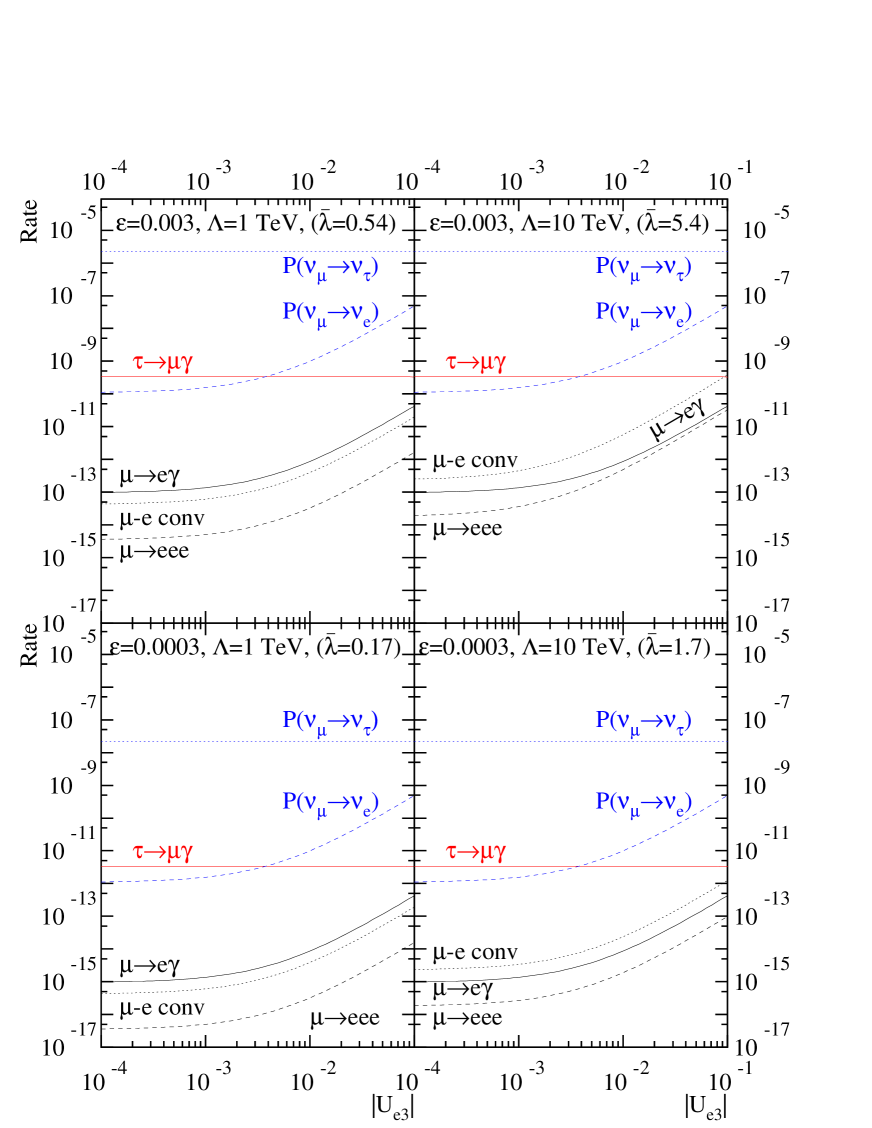
Figure 2: The most interesting leptonic observables as a function of $|U_{e3}|$, for $\delta=5$, $\epsilon=0.003$ (top) or 0.0003 (bottom), and $\Lambda=1$ TeV (left) or 10 TeV (right). We assume $\Delta m^{2}_{{\rm sun}}/\Delta m^{2}_{{\rm atm}}=10^{-2}$, $|U_{\mu 3}/U_{\tau 3}|^{2}=1$, $|U_{e2}/U_{e1}|^{2}=2/3$ (i.e., maximal mixing in the atmospheric sector and the LMA solution to the solar neutrino puzzle), no CP-violation in the neutrino mixing matrix, and hierarchical neutrino masses ($m_{1}^{2}\ll m_{2}^{2}\ll m_{3}^{2}$). Note that $\bar{\lambda}$ is the largest Yukawa coupling, $P(\nu_{i}\rightarrow\nu_{j})$ is the neutrino conversion probability at very short baselines, and the $\mu\to e$ conversion rate is computed for ${}^{27}{\rm Al}$.

$\mu\rightarrow e\bar{e}e$ and $\mu\rightarrow e$ conversion in nuclei

Unlike the $\ell_{i}\rightarrow\ell_{j}\gamma$ decays, these rare leptonic processes are more dependent on the unknown ultraviolet details of the models, but still a few interesting results can be obtained.

In $\mu\rightarrow e\bar{e}e$ process, several operators may contribute significantly (see the Appendix for detailed expressions). First of all, the $\mu\rightarrow e\gamma$ magnetic penguin operator contribution to $\mu\rightarrow e\bar{e}e$ is enhanced by $\ln(m_{\mu}/m_{e})$, which is a consequence of a collinear divergence of the electron-positron pair in the $m_{e}\rightarrow 0$ limit. Second, the $Z$ and photon penguin diagrams are enhanced by an ultraviolet divergence $\sim\ln(\Lambda/m_{W})$. When $\Lambda$ is significantly larger than $m_{W}$, this log-enhancement is important. Finally, as discussed after Eq. (4.2), the $Z$-penguin and box contributions contain $\bar{\lambda}^{4}$-terms. If the higher-dimensional KK neutrinos are coupled strongly enough such that $\bar{\lambda}>g$, then the $\bar{\lambda}^{4}$-terms may dominate over the other contributions to BR$(\mu\rightarrow e\bar{e}e)$.

In light of this discussion, the ratio of branching ratios BR$(\mu\rightarrow e\bar{e}e)$/BR$(\mu\rightarrow e\gamma)$, in which the overall $\epsilon^{2}$ dependence in both processes cancels out, can be written as

$$\frac{{\rm BR}(\mu\rightarrow e\bar{e}e)}{{\rm BR}(\mu\rightarrow e\gamma)}\approx C_{\mu\rightarrow e\gamma}+C_{\ln\Lambda}+C_{\bar{\lambda}}.$$ (4.13)

Here, $C_{\mu\rightarrow e\gamma}$ is the contribution from the $\mu\rightarrow e\gamma$ magnetic penguin operator

$$C_{\mu\rightarrow e\gamma}=\frac{\alpha}{3\pi}\left(\ln\frac{m^{2}_{\mu}}{m^{2}_{e}}-\frac{11}{4}\right)=6\times 10^{-3}.$$ (4.14)

The second term $C_{\ln\Lambda}$ contains the $\ln\Lambda/m_{W}$ contributions from the $Z$ and photon penguin diagrams of $\mu\rightarrow e\bar{e}e$. For example, the $Z$-penguin diagram leads to

$$C_{\ln\Lambda}\sim\frac{3\alpha}{8\pi}\left(3-\frac{2}{\sin^{2}\theta_{W}}+\frac{1}{2\sin^{2}\theta_{W}}\right)\left(\ln\frac{\Lambda^{2}}{m^{2}_{W}}-\frac{2}{\delta-2}-\frac{5}{3}\right)^{2}\sim 10^{-3}\left(\ln\frac{\Lambda^{2}}{m^{2}_{W}}-\frac{2}{\delta-2}-\frac{5}{3}\right)^{2}.$$ (4.15)

We find that $C_{\ln\Lambda}=0.03$ ($0.2$) for $\delta=5$ and $\Lambda=1$ TeV ($10$ TeV), when all ln terms present in the $Z$ and photon penguin diagrams are included.

The last term in Eq.(4.13), $C_{\bar{\lambda}}$, contains the contributions from $\bar{\lambda}^{4}$ terms in the $Z$-penguin and box diagrams:

$$C_{\bar{\lambda}}\propto\left(\frac{\bar{\lambda}}{g}\right)^{4}\frac{\left|U_{e2}U_{\mu 2}^{*}({\Delta m^{2}_{{\rm sun}}}/{\Delta m^{2}_{{\rm atm}}})^{2}+U_{e3}U_{\mu 3}^{*}\right|^{2}}{\left|U_{e2}U_{\mu 2}^{*}({\Delta m^{2}_{{\rm sun}}}/{\Delta m^{2}_{{\rm atm}}})^{\phantom{2}}+U_{e3}U_{\mu 3}^{*}\right|^{2}}.$$ (4.16)

When $|U_{e3}|$ is small, $C_{\bar{\lambda}}$ is small (suppressed by the small ratio of neutrino mass-squared differences squared). On the other hand, if $|U_{e3}|$ is sufficiently large, $C_{\bar{\lambda}}$ may in fact be the dominant contribution to $\mu\rightarrow e\bar{e}e$ due to the potentially large $(\bar{\lambda}/g)^{4}$ enhancement. Numerically, $C_{\bar{\lambda}}=0.6$ for $\Lambda=10$ TeV, $|U_{e3}|=0.1$, and $\epsilon=0.003$, which corresponds to $\bar{\lambda}=5.4$.

Because of the contributions $C_{\ln\Lambda}$ and $C_{\bar{\lambda}}$, the ratio BR$(\mu\rightarrow e\bar{e}e)$/BR$(\mu\rightarrow e\gamma)$ can be significantly larger than $10^{-1}$ if $\Lambda\,\raise 1.29167pt\hbox{$>$\kern-7.5pt\lower 4.30554pt\hbox{$\sim$}}\,1$ TeV or $\bar{\lambda}>g$. This is very different from predictions for lepton flavour violating processes from SUSY models with slepton flavour mixing, in which the contribution $C_{\mu\rightarrow e\gamma}$ is almost always dominant [40] and therefore BR$(\mu\rightarrow e\bar{e}e)$/BR$(\mu\rightarrow e\gamma)\simeq 6\times 10^{-3}$. Large contributions to BR$(\mu\rightarrow e\bar{e}e)$ may be obtained in SUSY models with $R$-parity violation [41].

The $\mu\rightarrow e$ conversion rate in nuclei behaves similarly to the $\mu\rightarrow e\bar{e}e$ branching ratio: for $\Lambda\gg m_{W}$, the log-enhancement in $Z$ and photon penguin diagrams is important and perhaps dominant, while if $\bar{\lambda}>g$, the $\bar{\lambda}^{4}$ term in the $Z$-penguin and box contributions can be significant. In both $\mu\rightarrow e\bar{e}e$ and $\mu\rightarrow e$ conversion in nuclei, the $Z$-penguin contribution tends to dominate because of the $\ln\Lambda$ and $\bar{\lambda}$ terms. When this is the case, the ratio R$(\mu\rightarrow e)$/BR$(\mu\rightarrow e\bar{e}e)$ does not depend on the unknown ultraviolet details of the models. We verified numerically that the ratio is almost constant, varying in the range 10–13 in the case of $\mu\to e$ conversion in ²⁷Al, and 20–25 in ⁴⁸Ti, in a large region of the parameter space. This feature is a definite prediction of the models under consideration. Again, the situation is different from SUSY models with slepton flavor mixing, where one expects R$(\mu\rightarrow e)$/BR$(\mu\rightarrow e\bar{e}e)\,\raise 1.29167pt\hbox{$<$\kern-7.5pt\lower 4.30554pt\hbox{$\sim$}}\,1$.

Figure 2 shows the branching ratio of $\mu\rightarrow e\bar{e}e$ and the rate for $\mu\to e$ conversion in ²⁷Al as a function of $|U_{e3}|$ for different values of $\Lambda$ and $\epsilon$ (we also fix $\delta=5$). All of the features we have discussed can be readily observed. First, one can clearly see that R$(\mu\rightarrow e~{}{\rm in~{}^{27}Al})$/BR$(\mu\rightarrow e\bar{e}e)$ is roughly constant ($\sim 10$) for all the depicted values of $\epsilon$ and $\Lambda$. Second, at small values of $|U_{e3}|$ (where the $\bar{\lambda}^{4}$ terms are negligible), the effect of the $\ln(\Lambda/m_{W})$ enhancement is visible: at $\Lambda=1$ TeV, BR$(\mu\to e\gamma)>$R$(\mu\rightarrow e~{}{\rm in~{}^{27}Al})$, while at $\Lambda=10$ TeV the situation is reversed. Finally, the $\bar{\lambda}^{4}$ enhancement is also clear if one compares R$(\mu\rightarrow e~{}{\rm in~{}^{27}Al})$/BR$(\mu\to e\gamma)$ and BR$(\mu\rightarrow e\bar{e}e)$/BR$(\mu\to e\gamma)$ at small and large values of $|U_{e3}|$, for $\bar{\lambda}$ large. This behavior is more easily observed for $\epsilon=0.003$ and $\Lambda=10$ TeV. Indeed, we have verified that at even larger values of $\bar{\lambda}$, BR$(\mu\rightarrow e\bar{e}e)$ exceeds BR$(\mu\to e\gamma)$. Note also that, for all values of $\epsilon$ and $\Lambda$ depicted in Fig. 2, the rate for $\mu\to e$ conversion in ²⁷Al is larger than the proposed sensitivity reach of the MECO experiment [42], even in the limit of small $|U_{e3}|$ (assuming the LMA solution to the solar neutrino puzzle).

Finally, we point out that, in general, the “atmospheric” and “solar” contributions to $\mu\to e\bar{e}e$ have different CP-violating phases. Furthermore, their relative weight in the magnetic penguin operator is different from their relative weight in the four-fermion operators in Eq. (4.2), unless $\bar{\lambda}\ll g$. If the “atmospheric” and “solar” contributions are comparable, the interference between them produces observable CP-violating effects in polarized $\mu\to e\bar{e}e$ decays [43].

$g-2$ of the muon

As derived in the Appendix (see also [44]), the contribution of the KK tower of neutrinos to the muon anomalous magnetic moment is

$$\delta a_{\mu} = -\frac{g^{2}}{32\pi^{2}}\frac{m^{2}_{\mu}}{m^{2}_{W}}\epsilon\sum_{j}\left|U_{\mu j}\right|^{2}\frac{m^{2}_{\nu j}}{\Delta m^{2}_{{\rm atm}}}\simeq-10^{-9}\epsilon.$$ (4.17)

Here we have assumed maximal mixing in the solar sector and neglected $U_{e3}$ and $\Delta m^{2}_{{\rm sun}}/\Delta m^{2}_{\rm atm}$ corrections. Note that the sign of the effect is negative, in contrast to the BNL experimental result [45], that claims a discrepancy $\delta a_{\mu}=+(4.3\pm 1.6)\times 10^{-9}$ with respect to SM predictions (afflicted, however, by significant hadronic uncertainties). On the other hand, the present bounds on the $\epsilon_{ij}$ parameters already require in a model-independent way that the right-handed neutrino correction to $g-2$ is smaller than the theoretical uncertainty in the hadronic SM contributions. If, in the future, more precise experimental and theoretical results establish the presence of a non SM correction to $g-2$, extra dimensional models could still account for it by invoking ad-hoc dimension-six operators like $\frac{1}{\Lambda^{2}}(\bar{L}\tau^{a}\sigma_{\mu\nu}D/~{}L)W^{a}_{\mu\nu}$ with $\Lambda\approx(3\div 4)\,{\rm TeV}$. There is no direct contradiction between such non renormalizable operators and bounds from the more sensitive precision data.

Non minimal flat models and warped models

Nonminimal flat models and models with warped extra dimensions do not allow one to relate the coefficients of the dimension-six effective operators to the parameters in the neutrino Dirac mass matrix. For this reason, it is not possible to make interesting predictions. In non minimal flat models (B) and in warped models the naïve expectation is that all $\epsilon_{ij}$ are comparable, but is easy to avoid this conclusion. It is useful to estimate the $\ell_{i}\to\ell_{j}\gamma$ decays in terms of the $\epsilon_{ij}$ parameters defined in Eq. (1.1). Up to order one uncomputable factors, $\ell_{i}\to\ell_{j}\gamma$ experiments give the following bounds

$$|\epsilon_{e\mu}|\,\raise 1.29167pt\hbox{$<$\kern-7.5pt\lower 4.30554pt\hbox{$\sim$}}\,10^{-4},\qquad|\epsilon_{e\tau}|,|\epsilon_{\mu\tau}|\,\raise 1.29167pt\hbox{$<$\kern-7.5pt\lower 4.30554pt\hbox{$\sim$}}\,10^{-1}.$$ (4.18)

Such bounds prohibit the interpretation of the LSND anomaly [13] as due to $\epsilon_{e\mu}$, as discussed in the previous section. In fact, the present bound on $\epsilon_{e\mu}$ is so strong that it will be hard to observe its effects in $\nu_{e}\leftrightarrow\nu_{\mu}$ transitions, even with a neutrino factory.

$$\begin{array}[]{|c|lclc|lclc|}\hline\cr&\vrule\lx@intercol\hfil\hbox{present {\bf bounds} from experiments with}\hfil\lx@intercol\vrule\lx@intercol&\vrule\lx@intercol\hfil\hbox{future {\bf sensitivity} from experiments with}\hfil\lx@intercol\vrule\lx@intercol\\ \hline\cr&\vrule\lx@intercol\hfil\hbox{neutrinos}\hfil\lx@intercol&\vrule\lx@intercol\hfil\hbox{charged leptons}\hfil\lx@intercol&\vrule\lx@intercol\hfil\hbox{neutrinos}\hfil\lx@intercol&\vrule\lx@intercol\hfil\hbox{charged leptons}\hfil\lx@intercol\vrule\lx@intercol\\ \hline\cr|\epsilon_{e\mu}|&<0.05&\hbox{({\sc Karmen})}&\,\raise 1.29167pt\hbox{$<$\kern-7.5pt\lower 4.30554pt\hbox{$\sim$}}\,10^{-4}&(\mu\to e\gamma)&\sim 10^{-4}&\hbox{($\nu$ factory)}&\sim 10^{-5\div 6}&(\mu~{}{\rm decays})\\ |\epsilon_{e\tau}|&<0.09&\hbox{(NOMAD)}&\,\raise 1.29167pt\hbox{$<$\kern-7.5pt\lower 4.30554pt\hbox{$\sim$}}\,10^{-1}&(\tau\to e\gamma)&\sim 10^{-4}&\hbox{($\nu$ factory)}&\sim 10^{-1\div 2}&(\tau\to e\gamma)\\ |\epsilon_{\mu\tau}|&<0.013&\hbox{(NOMAD)}&\,\raise 1.29167pt\hbox{$<$\kern-7.5pt\lower 4.30554pt\hbox{$\sim$}}\,10^{-1}&(\tau\to\mu\gamma)&\sim 10^{-4}&\hbox{($\nu$ factory)}&\sim 10^{-1\div 2}&(\tau\to\mu\gamma)\\ \epsilon_{ee}&<0.025&\hbox{(reactors)}&\,\raise 1.29167pt\hbox{$<$\kern-7.5pt\lower 4.30554pt\hbox{$\sim$}}\,10^{-3}&(Z\hbox{ data})&\sim 10^{-3}&\hbox{($\nu$ factory)}&\sim 10^{-3\div 4}&(Z\hbox{ data})\\ \epsilon_{\mu\mu}&~{}~{}~{}\hbox{---}&&\,\raise 1.29167pt\hbox{$<$\kern-7.5pt\lower 4.30554pt\hbox{$\sim$}}\,10^{-3}&(Z\hbox{ data})&\sim 10^{-3}&\hbox{($\nu$ factory)}&\sim 10^{-3\div 4}&(Z\hbox{ data})\\ \epsilon_{\tau\tau}&~{}~{}~{}\hbox{---}&&\,\raise 1.29167pt\hbox{$<$\kern-7.5pt\lower 4.30554pt\hbox{$\sim$}}\,10^{-2}&(Z\to\nu\bar{\nu})&~{}~{}~{}\hbox{---}&&\sim 10^{-3}&(Z\to\nu\bar{\nu})\\ \hline\cr\end{array}$$

Table 1: Bounds and future sensitivity reaches for the $\epsilon_{ij}$ coefficients defined by Eq. (1.1).

5 Conclusions

We have shown that the various minimal and non minimal models with right-handed neutrinos in flat or warped extra dimension are described at low energy by neutrino masses plus a specific set of dimension six operators. Up to order one factors (that are anyhow uncomputable since these models are not renormalizable), flavour conserving effects are described by three positive numbers $\epsilon_{ee},~{}\epsilon_{\mu\mu},~{}\epsilon_{\tau\tau}$, and flavour-violating effects are described by three complex numbers $\epsilon_{e\mu},~{}\epsilon_{e\tau},~{}\epsilon_{\mu\tau}$, defined in Eq. (1.1). This gives rise to several relations between non-SM effects in neutrino observables and in lepton flavour-violating processes. Effects in charged leptons are suppressed by a one loop factor with respect to effects in neutrinos:

$$P(\nu_{i}\to\nu_{j};L\approx 0)\sim|\epsilon_{ij}^{2}|,\qquad{\rm BR}(\ell_{i}\to\ell_{j}\gamma)\sim|e\epsilon_{ij}/4\pi|^{2},\qquad(i\neq j).$$ (5.1)

Present bounds from neutrino experiments and from charged lepton processes are summarized in Table 1. Due to the loop factor, detectable neutrino effects are compatible with lepton flavour violating bounds, unlike what is obtained with a generic larger set of SU(2)_L-invariant dimension six operators, where neutrino and charged lepton effects both arise at tree level. Values of $\epsilon_{ij}\,\raise 1.29167pt\hbox{$>$\kern-7.5pt\lower 4.30554pt\hbox{$\sim$}}\,10^{-4}$ (including possible CP-violating phases) will be probed by future neutrino experiments. The importance of $\mu\to e\bar{e}e$ and $\mu\to e$ conversion relative to $\mu\to e\gamma$ can be enhanced, with respect to the usual magnetic-penguin dominance approximation, if the right-handed neutrino is strongly coupled or if the cut-off of the theory is significantly larger than the $W$ mass.

All these effects can be generated in four dimensions by adding “right-handed neutrinos” with TeV-scale masses and order one Yukawa couplings, but such choice of parameters is not motivated by neutrino masses. On the contrary, extra-dimensional models that try to address the hierarchy problem and to generate neutrino masses give an order-of-magnitude expectation for the $\epsilon_{ij}$ parameters of $\epsilon_{ij}\sim\ell_{\delta}(v/\,{\rm TeV})^{2}\sim 10^{-{\rm few}}$ where $\ell_{\delta}$ is a loop factor in $\delta$ dimensions. Therefore, these models are compatible with a “natural” value for the fundamental scale.

In the flat minimal model, the six $\epsilon_{ij}$ parameters are related and can be expressed in terms of a single unknown $\epsilon$, see Eq. (3.9). The value of $\epsilon$ is at present constrained by LEP and neutrino experiments ($\epsilon\,\raise 1.29167pt\hbox{$<$\kern-7.5pt\lower 4.30554pt\hbox{$\sim$}}\,0.004$) and by the $\mu\to e\gamma$ decay, see Eqs. (4.10) and (4.12). Improvements in the sensitivity on rare muon processes and measurements at a future neutrino factory will significantly extend the probe on the hypothesis of an extra-dimensional origin of neutrino masses.

Acknowledgments

We thank Paolo Criminelli, Riccardo Rattazzi, Serguey Petcov and Alexei Smirnov for useful discussions.

Note added

The NuTeV collaboration [48] has recently reported a 3-$\sigma$ anomaly in $\nu_{\mu}$-nucleon scattering, that can interpreted as due to a ratio between the $\bar{\nu}_{\mu}Z\nu_{\mu}$ and the $\bar{\nu}_{\mu}W\mu$ couplings $(0.58\pm 0.21)\%$ lower than in the SM. Since LEP found that the $Z$ couplings to other fermions agree with SM predictions at the per-mille level, the NuTeV anomaly could be due to physics beyond the SM that mainly affects the neutrinos. This is what happens in the extra dimensional models considered here, where the $\bar{\nu}_{\mu}Z\nu_{\mu}$ coupling is $1-\epsilon_{\mu\mu}$ smaller than in the SM, while the $\bar{\nu}_{\mu}W\mu$ coupling is smaller by only $1-{\epsilon_{\mu\mu}}/{2}$ (see section 3). The NuTeV anomaly could be fitted by $\epsilon_{\mu\mu}=0.0116\pm 0.0042$. This value gives a reduction of the $Z\to\nu\bar{\nu}$ width compatible with the LEP measurement, 2-$\sigma$ lower than its SM prediction (see footnote in page 7). However, the fact that the charged current is also modified imposes severe constraints (the strongest bound, $\epsilon_{\mu\mu}+\epsilon_{ee}\,\raise 1.29167pt\hbox{$<$\kern-7.5pt\lower 4.30554pt\hbox{$\sim$}}\,0.002$, comes from a comparision of the muon lifetime with precision electroweak data), which prevent a clean explaination the NuTeV anomaly.

Appendix A Integrating out right-handed neutrinos

In this Appendix, we present in detail the expressions for the effective operators that mediate rare muon processes and the muon anomalous magnetic moment when the entire tower of KK right-handed neutrinos (up to some arbitrary cut-off) is integrated out. The computation is done in the minimal flat model, but can be easily generalized to other cases of interest.

Magnetic moment type operator for $\mu\rightarrow e\gamma$

The rare decay $\mu\rightarrow e\gamma$ takes place at the one-loop level. The following magnetic moment operator is generated when all one-loop diagrams involving KK neutrinos are added.

$${\cal L}=m_{\mu}\bar{e}\sigma_{\alpha\beta}(A_{L}P_{L}+A_{R}P_{R})\mu F^{\alpha\beta}+{\rm h.c.}$$ (A.1)

where $A_{L}=0$,

$$A_{R} = \frac{eg^{2}}{64\pi^{2}}\frac{1}{m^{2}_{W}}\sum_{\vec{n},j}V_{e\vec{n}}^{j}V_{\mu\vec{n}}^{j*}G_{\gamma}(m^{(j)2}_{\vec{n}}/m^{2}_{W}),$$ (A.2)

$$G_{\gamma}(x) = -\frac{x(1-6x+3x^{2}+2x^{3}-6x^{2}\ln x)}{4(1-x)^{4}}.$$ (A.3)

Here the summation of all KK modes, which are labeled by the generation $j$ and the integer vector $\vec{n}$ in the $\delta$-extra dimension, are taken into account. $m^{(j)}_{\vec{n}}$ is the mass of a KK neutrino labeled by $j$ and ${\vec{n}}$, and $V_{i\vec{n}}^{j}$ is defined as $V_{i{\vec{n}}}^{j}\equiv U_{ij}V_{L}^{j{\vec{n}}}$, where $U_{ij}$ is the standard active neutrino mixing matrix and $V_{L}^{j\vec{n}}$ is the active-KK mixing matrix. When $m^{(j)}_{\vec{n}}\gg m_{\nu j}$, $m^{(j)2}_{\vec{n}}\approx{\vec{n}}^{2}/R^{2}$ and $V_{L}^{j\vec{n}}\approx m_{\nu j}/m^{(j)}_{\vec{n}}$. The branching ratio for $\mu\rightarrow e\gamma$ is given by

$$\frac{{\rm BR}(\mu\rightarrow e\gamma)}{{\rm BR}(\mu\rightarrow e\nu_{e}\nu_{\mu})} = \frac{48\pi^{2}|A_{R}|^{2}}{G_{F}^{2}}=\frac{3\alpha}{2\pi}\left|\sum_{\vec{n},j}V_{e\vec{n}}^{j}V^{j*}_{\mu\vec{n}}G_{\gamma}(m^{(j)2}_{\vec{n}}/m^{2}_{W})\right|^{2}.$$ (A.4)

The same expressions can be used for $\tau\rightarrow l\gamma$ after replacing $m_{\mu}\rightarrow m_{\tau}$, $V^{j*}_{\mu{\vec{n}}}\rightarrow V^{j*}_{\tau{\vec{n}}}$, $V^{j}_{e{\vec{n}}}\rightarrow V^{j}_{l{\vec{n}}}$, and ${\rm BR}(\mu\rightarrow e\nu_{e}\nu_{\mu})\rightarrow{\rm BR}(\tau\rightarrow l\nu_{l}\nu_{\tau})$, for $l=e$ or $\mu$.

Next, we sum over all KK modes. In models with large extra dimensions, the sum over the KK states can be accurately replaced by an integral

$$\sum_{\vec{n}}^{|\vec{n}|<\Lambda R}f\left(\frac{{\vec{n}}^{2}}{{R}^{2}}\right)\rightarrow S_{\delta}R^{\delta}\int_{0}^{\Lambda}dE\,E^{\delta-1}f(E^{2}),$$ (A.5)

where $f$ is any function and $S_{\delta}=2\pi^{\delta/2}/\Gamma(\delta/2)$. The cut off $\Lambda$ is expected to be of order of the fundamental scale $\Lambda\sim\bar{M}_{D}$. Therefore,

$$\sum_{\vec{n},j}V_{e\vec{n}}^{j}V_{\mu\vec{n}}^{j*}G_{\gamma}(m_{\vec{n}}^{(j)2}/m^{2}_{W}) \approx \sum_{j}U_{ej}U_{\mu j}^{*}S_{\delta}R^{\delta}\int_{0}^{\Lambda}dE\,E^{\delta-1}\left|\frac{m_{\nu j}}{E}\right|^{2}G_{\gamma}(E^{2}/m^{2}_{W})$$ (A.6)

$$\approx \sum_{j}U_{ej}U_{\mu j}^{*}m_{\nu j}^{2}S_{\delta}R^{\delta}\int_{0}^{\Lambda}dE\,E^{\delta-3}\left(-\frac{1}{2}\right)$$

$$= -\frac{1}{2}\left[\frac{S_{\delta}}{\delta-2}\left(\frac{\Lambda}{\bar{M}_{D}}\right)^{\delta}\left(\frac{\bar{M}_{4}}{\bar{M}_{D}}\right)^{2\delta/\gamma}\frac{1}{\Lambda^{2}}\frac{1}{(2\pi)^{\delta}}\right]\sum_{j}U_{ej}U_{\mu j}^{*}m_{\nu j}^{2}.$$

We only consider $\delta>2$. Note that we have used the definition of the reduced Planck mass, Eq. (2.7). The term in the square brackets equals $\epsilon/\Delta m^{2}_{{\rm atm}}$ (as defined in Sec. 2).

4-fermion operators for $\mu\rightarrow e\bar{e}e$ and $\mu\rightarrow e$ conversion in nuclei

In addition to the magnetic moment type operator Eq. (A.2), the following 4-fermion operator contributes to the $\mu\rightarrow e\bar{e}e$ process:

$$\cal{L} = \bar{e}\gamma_{\alpha}P_{L}\mu~{}~{}\bar{e}\gamma^{\alpha}\left\{\left(A_{\gamma}+g^{e}_{L}A_{Z}+A_{B}\right)P_{L}+\left(A_{\gamma}+g^{e}_{R}A_{Z}\right)P_{R}\right\}e+{\rm h.c.}$$ (A.7)

Here $g^{f}_{L(R)}=T^{f}_{3L(R)}-Q_{f}\sin^{2}\theta_{W}$ ($g^{e}_{L}=-1/2+\sin^{2}\theta_{W}$ and $g^{e}_{R}=\sin^{2}\theta_{W}$). The coefficients $A_{\gamma}$, $A_{Z}$, and $A_{B}$ correspond to contributions from photon penguin, $Z$-penguin, and box diagrams, respectively. Explicitly,

$$A_{\gamma} = -\frac{e^{2}g^{2}}{32\pi^{2}}\frac{1}{m^{2}_{W}}\sum_{\vec{n},j}V_{e\vec{n}}^{j}V^{j*}_{\mu\vec{n}}F_{\gamma}(m^{(j)2}_{\vec{n}}/m^{2}_{W}),$$ (A.8)

$$A_{Z} = -\frac{g^{4}}{64\pi^{2}}\frac{1}{m^{2}_{W}}\bigg{\{}\sum_{\vec{n},j}V_{e\vec{n}}^{j}V_{\mu\vec{n}}^{j*}F_{Z}(m^{(j)2}_{\vec{n}}/m^{2}_{W})$$ (A.9)

$$+\sum_{\vec{n},\vec{m},j}V_{e\vec{n}}^{j}V_{L}^{j\vec{n}*}V_{L}^{j\vec{m}*}V_{\mu\vec{m}}^{j*}G_{Z}(m^{(j)2}_{\vec{n}}/m^{2}_{W},m^{(j)2}_{\vec{m}}/m^{2}_{W})\bigg{\}},$$

$$A_{B} = -\frac{g^{4}}{64\pi^{2}}\frac{1}{m^{2}_{W}}\sum_{\vec{n},\vec{m},i,j}V_{e\vec{n}}^{i}V_{\mu\vec{n}}^{i*}V_{e\vec{m}}^{j}V_{e\vec{m}}^{j*}G_{B}(m^{(i)2}_{\vec{n}}/m^{2}_{W},m^{(j)2}_{\vec{m}}/m^{2}_{W}),$$ (A.10)

$$F_{\gamma}(x) = -\frac{x\left\{12-11x-8x^{2}+7x^{3}+2x(x^{2}-10x+12)\ln{x}\right\}}{12(1-x)^{4}},$$ (A.11)

$$F_{Z}(x) = \frac{5x(1-x+x\ln{x})}{(1-x)^{2}},$$ (A.12)

$$G_{Z}(x,y) = \frac{1}{x-y}\left\{\frac{x^{2}(1-y)\ln{x}}{1-x}-\frac{y^{2}(1-x)\ln{y}}{1-y}\right\},$$ (A.13)

$$G_{B}(x,y) = \frac{1}{x-y}\left[\left(1+\frac{xy}{4}\right)\left\{\frac{1}{1-x}+\frac{x^{2}\ln{x}}{(1-x)^{2}}-\frac{1}{1-y}-\frac{y^{2}\ln{y}}{(1-y)^{2}}\right\}\right.$$ (A.14)

$$\left.-2xy\left\{\frac{1}{1-x}+\frac{x\ln{x}}{(1-x)^{2}}-\frac{1}{1-y}-\frac{y\ln{y}}{(1-y)^{2}}\right\}\right].$$

The branching ratio for $\mu\rightarrow e\bar{e}e$ process is

$${\rm BR}(\mu\rightarrow e\bar{e}e) = \frac{1}{8G_{F}^{2}}\bigg{[}\left|A_{\gamma}+g_{R}^{e}A_{Z}\right|^{2}+2\left|A_{\gamma}+g_{L}^{e}A_{Z}+A_{B}\right|^{2}+32\left|eA_{R}\right|^{2}\left(\ln\frac{m^{2}_{\mu}}{m^{2}_{e}}-\frac{11}{4}\right)$$ (A.15)

$$+4eA_{R}\left\{3A_{\gamma}^{*}+(g_{R}^{e}+2g_{L}^{e})A_{Z}^{*}+2A_{B}^{*}\right\}+{\rm h.c.}\bigg{]}.$$

In addition to the magnetic moment type operator Eq. (A.2), the following 4-fermion operator contributes to $\mu\rightarrow e$ conversion in nuclei:

$$\cal{L} = \sum_{q=u,d}\bar{q}\gamma_{\alpha}q~{}~{}\bar{e}\gamma^{\alpha}\left(-Q_{q}A_{\gamma}+\frac{g^{q}_{L}+g^{q}_{R}}{2}A_{Z}+B_{B}^{q}\right)P_{L}\mu,$$ (A.16)

$$B^{d}_{B} = -\frac{g^{4}}{128\pi^{2}}\frac{1}{m^{2}_{W}}\sum_{\vec{n},i,j}V_{e\vec{n}}^{j}V_{\mu\vec{n}}^{j*}\left|V_{u_{i}d}\right|^{2}G_{B}(m^{(j)2}_{\vec{n}}/m^{2}_{W},m^{2}_{u_{i}}/m^{2}_{W}),$$ (A.17)

$$B^{u}_{B} = -\frac{g^{4}}{32\pi^{2}}\frac{1}{m^{2}_{W}}\sum_{\vec{n},j}V_{e\vec{n}}^{j}V_{\mu\vec{n}}^{j*}G_{B}(m^{(j)2}_{\vec{n}}/m^{2}_{W},0).$$ (A.18)

The $\mu\rightarrow e$ conversion rate is

$${\rm R}(\mu\rightarrow e) = \frac{\alpha^{3}}{4\pi^{2}}\frac{Z_{\rm eff}^{4}}{Z}\frac{|F(-m^{2}_{\mu})|^{2}m^{5}_{\mu}}{\Gamma_{\rm\mu-capt}}\bigg{|}(2Z+N)\left(\frac{g^{u}_{L}+g^{u}_{R}}{2}A_{Z}+B^{u}_{B}\right)$$ (A.19)

$$+(Z+2N)\left(\frac{g^{d}_{L}+g^{d}_{R}}{2}A_{Z}+B^{d}_{B}\right)-Z(2eA_{R}+A_{\gamma})\bigg{|}^{2},$$

where $\Gamma_{\rm\mu-capt}$ is the muon capture rate in nuclei of interest [46], $Z$ and $N$ are the proton and neutron numbers, respectively, $F(-m_{\mu}^{2})$ is the nuclear form factor and $Z_{\rm eff}$ is the nuclear effective charge [47]. Numerically, these nuclear parameters are $\Gamma_{\rm\mu-capt}=1.7\times 10^{-18}~{}{\rm GeV}$ $(4.6\times 10^{-19}~{}{\rm GeV})$, $Z_{\rm eff}=17.6$ $(11.6)$, and $|F(-m^{2}_{\mu})|=0.535$ $(0.64)$ for ${}^{48}_{22}{\rm Ti}$ (${}^{27}_{13}{\rm Al}$) [46, 47].

Summing over the KK states following the steps previously outlined, we obtain

$$A_{\gamma} \approx -\frac{e^{2}g^{2}}{64\pi^{2}}\frac{1}{m^{2}_{W}}\epsilon\sum_{j}U_{ej}U_{\mu j}^{*}\frac{m^{2}_{\nu j}}{\Delta m^{2}_{{\rm atm}}}\left\{\frac{7}{6}+\frac{1}{3}\left(\ln\frac{\Lambda^{2}}{m_{W}^{2}}-\frac{2}{\delta-2}\right)\right\},$$ (A.20)

$$A_{Z} \approx -\frac{g^{4}}{64\pi^{2}}\frac{1}{m_{W}^{2}}\epsilon\sum_{j}U_{ej}U_{\mu j}^{*}\frac{m^{2}_{\nu j}}{\Delta m^{2}_{{\rm atm}}}\left\{\epsilon J_{\delta}\frac{m_{\nu j}^{2}\Lambda^{2}}{\Delta m^{2}_{{\rm atm}}m^{2}_{W}}\right.$$ (A.21)

$$\left.+\left(3-2\epsilon\frac{m^{2}_{\nu j}}{\Delta m^{2}_{{\rm atm}}}\right)\left(\ln\frac{\Lambda^{2}}{m_{W}^{2}}-\frac{2}{\delta-2}\right)-5\right\},$$

$$A_{B} \approx -\frac{g^{4}}{64\pi^{2}}\frac{1}{m^{2}_{W}}\epsilon\sum_{j}U_{ej}U_{\mu j}^{*}\frac{m^{2}_{\nu j}}{\Delta m^{2}_{{\rm atm}}}\left\{\epsilon J_{\delta}\sum_{i}|U_{ei}|^{2}\frac{m^{2}_{\nu i}\Lambda^{2}}{\Delta m^{2}_{\rm atm}m_{W}^{2}}\right.$$ (A.22)

$$\left.+\epsilon\sum_{i}|U_{ei}|^{2}\frac{m^{2}_{\nu i}}{\Delta m^{2}_{{\rm atm}}}-1\right\},$$

$$B_{B}^{d} = -\frac{g^{4}}{64\pi^{2}}\frac{1}{m^{2}_{W}}\epsilon\sum_{j}U_{ej}U_{\mu j}^{*}\frac{m^{2}_{\nu j}}{\Delta m^{2}_{{\rm atm}}}\frac{|V_{td}|^{2}}{8}\frac{m^{2}_{\rm top}}{m^{2}_{W}}\left(\ln\frac{\Lambda^{2}}{m^{2}_{W}}-\frac{2}{\delta-2}\right),$$ (A.23)

$$B_{B}^{u} \sim ~{}{\rm small},$$ (A.24)

$$eA_{R} \approx -\frac{e^{2}g^{2}}{64\pi^{2}}\frac{1}{m_{W}^{2}}\frac{\epsilon}{2}\sum_{j}U_{ej}U_{\mu j}^{*}\frac{m_{\nu j}^{2}}{\Delta m^{2}_{{\rm atm}}}.$$ (A.25)

where $J_{\delta}\equiv(1-\delta/2)^{2}\int_{0}^{1}\int_{0}^{1}(zw)^{\delta/2-1}\ln(z/w)/(z-w)\,dz\,dw$, which is the number of order 1. Numerically, $J_{3}=0.23$, $J_{4}=0.43$, $J_{5}=0.55$, and $J_{6}=0.63$.

Note that, unlike the $\mu\rightarrow e\gamma$ case, most of the amplitudes depend not only on the neutrino mass-squared difference (which is directly measured by neutrino oscillation experiments), but also on the magnitude of the neutrino mass-squared.

Magnetic moment operator for muon $g-2$

The anomalous magnetic moment ($\delta a_{\mu}$) of the muon is defined as the coefficient of the effective operator

$${\cal L} = \frac{e}{4m_{\mu}}\delta a_{\mu}~{}\bar{\mu}\sigma_{\alpha\beta}\mu F^{\alpha\beta}.$$ (A.26)

The contribution to muon anomalous magnetic moment induced by massive KK modes is given by

$$\delta a_{\mu} = \frac{g^{2}}{16\pi^{2}}\frac{m^{2}_{\mu}}{m^{2}_{W}}\bigg{\{}\sum_{\vec{n},j}\left|V_{\mu\vec{n}}^{j}\right|^{2}f({m^{(j)2}_{\vec{n}}/m^{2}_{W}})-\frac{5}{6}\bigg{\}},$$ (A.27)

$$f(x) = \frac{10-43x+78x^{2}-49x^{3}+4x^{4}+18x^{3}\ln x}{12(1-x)^{4}}.$$ (A.28)

Note that we have subtracted the SM ($W,\nu$)-loop in order to calculate the new physics contribution. It is useful to separate the sum into the “massless” part (we neglect the effect of the small active neutrino masses) and the “massive” part. Using the unitarity of $V_{\mu M}^{j}$ and the fact that $f(0)=5/6$, we can rewrite

$$\delta a_{\mu} = \frac{g^{2}}{16\pi^{2}}\frac{m^{2}_{\mu}}{m^{2}_{W}}\sum_{\vec{n},j}\left|V_{\mu\vec{n}}^{j}\right|^{2}G_{\gamma}(m^{(j)2}_{\vec{n}}/m^{2}_{W}),$$ (A.29)

Here, the function $G_{\gamma}(x)\equiv f(x)-5/6$ is defined by Eq. (A.3). Summing over the KK states (see Eq. (A.6)) we obtain Eq. (4.17).

References

• [1] I. Antoniadis, Phys. Lett. B246 (1990) 377; J.D. Lykken, Phys. Rev. D54 (1996) 3693 (hep-th/9603133); N. Arkani-Hamed, S. Dimopoulos, G. Dvali, Phys. Lett. B429 (1998) 263 (hep-ph/9803315).
• [2] L. Randall, R. Sundrum, Phys. Rev. Lett. 83 (1999) 3370 (hep-ph/9905221).
• [3] S. Dimopoulos, talk given at the SUSY 1998 conference.
• [4] K.R. Dienes, E. Dudas, T. Gherghetta, Nucl. Phys. B557 (1999) 25 (hep-ph/9811428).
• [5] N. Arkani-Hamed et al, hep-ph/9811448.
• [6] Y. Grossman, M. Neubert, Phys. Lett. B474 (2000) 361 (hep-ph/9912408).
• [7] I. Antoniadis, C. Bachas, Phys. Lett. B450 (1999) 83 (hep-th/9812093).
• [8] R. Barbieri, P. Creminelli, A. Strumia, Nucl. Phys. B585 (2000) 28 (hep-ph/0002199).
• [9] A. Lukas, P. Ramond, A. Romanino, G.G. Ross, J.HEP 104 (2001) 10 (hep-ph/0011295). For earlier extra-dimensional models of the solar anomaly see e.g. G. Dvali, A. Yu Smirnov, Nucl. Phys. B563 (1999) 63 (hep-ph/9904211); R.N. Mohapatra, A. Perez-Lorenzana, S.J. Yellin, Phys. Rev. Lett. 87 (2001) 041601 (hep-ph/0010353); and references therein.
• [10] The SuperKamiokande collaboration, hep-ex/0105023.
• [11] The SuperKamiokande collaboration, Phys. Rev. Lett. 86 (2001) 5651 (hep-ex/0103032).
• [12] The SNO collaboration, nucl-ex/0106015.
• [13] The LSND collaboration, hep-ex/0104049.
• [14] A.E. Faraggi, M. Pospelov, Phys. Lett. B458 (1999) 237 (hep-ph/9901299); R. Kitano, Phys. Lett. B481 (2000) 39 (hep-ph/0002279); T.P. Cheng, L. Li, Phys. Lett. B502 (2001) 152 (hep-ph/0101068).
• [15] A. Ioannisian, A. Pilaftsis, Phys. Rev. D62 (2000) 066001 (hep-ph/9907522).
• [16] G.F. Giudice, R. Rattazzi, J.D. Wells, Nucl. Phys. B544 (1999) 3 (hep-ph/9811291); E.A. Mirabelli, M. Perelstein, M.E. Peskin, Phys. Rev. Lett. 82 (1999) 2236 (hep-ph/9811337); T. Han, J.D. Lykken, R. Zhang, Phys. Rev. D59 (1999) 105006 (hep-ph/9811350).
• [17] M. Gogberashvili, hep-ph/9812296.
• [18] W. D. Goldberger, M. B. Wise, Phys. Rev. D60 (1999) 107505 (hep-ph/9907218).
• [19] J. Maldacena, Adv. Theor. Math. Phys. 2 (1998) 231 (hep-th/9711200); E. Witten, talk at ITP conference ‘New Dimensions in Field Theory and String Theory’, available at the interned address www.itp.ucsb.edu/online/susy c99/discussion.
• [20] C. Csaki, J. Erlich, C. Grojean, Nucl. Phys. B604 (2001) 312 (hep-th/0012143).
• [21] J. Maxwell, A Treatise on Electricity and Magnetism (1873).
• [22] L. Wolfenstein, Phys. Rev. D17 (1978) 2369; S.P. Mikheyev, A. Yu Smirnov, Sovietic Jour. Nucl. Phys. 42 (1985) 913; P. Langacker, S.T. Petcov, G. Steigman, S. Toshev, Nucl. Phys. B282 (1987) 589.
• [23] G.L. Fogli, E. Lisi, A. Marrone, G. Scioscia, Phys. Rev. D60 (1999) 53006 (hep-ph/9904248).
• [24] K. Agashe, N.G. Deshpande, G.H. Wu, Phys. Lett. B489 (2000) 367 (hep-ph/0006122).
• [25] The Nomad collaboration, hep-ex/0106102. See also the Chorus collaboration, Phys. Lett. B497 (2001) 8.
• [26] The Karmen collaboration, Nucl. Phys. Proc. Suppl. 91 (2000) 191 (hep-ex/0008002).
• [27] The Chooz collaboration, Phys. Lett. B466 (1999) 415 (hep-ex/9907037); see also the Palo Verde collaboration, Phys. Rev. Lett. 84 (2000) 3764 (hep-ex/9912050).
• [28] Y. Declais et al, Nucl. Phys. B434 (1995) 503.
• [29] LEP and SLD collaborations, hep-ex/0103048.
• [30] For a review on $\tau$ decays see e.g. A. Pich, Nucl. Phys. Proc. Suppl. 98 (2001) 385 (hep-ph/0012297). See also [15].
• [31] M. Mangano et al., nu-DIS working group of the ECFA-CERN neutrino factory study group, hep-ph/0105155.
• [32] Y. Grossman, Phys. Lett. B359 (1995) 141 (hep-ph/9507344); M.C. Gonzalez-Garcia, Y. Grossman, A. Gusso, Y. Nir, hep-ph/0105159 and references therein.
• [33] F.J. Botella, C.S. Lim, W.J. Marciano, Phys. Rev. D35 (1987) 896.
• [34] A.M. Gago, M.M. Guzzo, H. Nunokawa, W.J. Teves, R.Z. Funchal, hep-ph/0105196.
• [35] C. Lunardini, A.Yu Smirnov, Phys. Rev. D63 (2001) 073009 (hep-ph/0009356).
• [36] G. Barenboim, G.C. Branco, A. de Gouvêa, M.N. Rebelo, hep-ph/0104312
• [37] F. Vissani, D. Delepine, hep-ph/0106287.
• [38] L. Barkov et al., research proposal to PSI, available at meg.icepp.s-tokyo.ac.jp.
• [39] For global post-SNO analyses of the solar neutrino data see G.L. Fogli, E. Lisi, D. Montanino, A. Palazzo, hep-ph/0106247; A. Bandyopadhyay, S. Choubey, S. Goswami, K. Kar, hep-ph/0106264; J.N. Bahcall, M.C. Gonzalez-Garcia, C. Peña-Garay, hep-ph/0106258; the addendum to P. Creminelli, G. Signorelli, A. Strumia, hep-ph/0102234.
• [40] Y. Kuno, Y. Okada, Rev. Mod. Phys. 73 (2001) 151 (hep-ph/9909265), and references therein.
• [41] A. de Gouvêa, S. Lola, K. Tobe, Phys. Rev. D63 (2001) 035004 (hep-ph/0008085).
• [42] MECO collaboration, BNL proposal AGS P940, available at meco.ps.uci.edu.
• [43] Y. Okada, K. Okumura, Y. Shimizu, Phys. Rev. D58 (1998) 51901 (hep-ph/9708446).
• [44] G.C. McLaughlin, J.N. Ng, Phys. Lett. B493 (2000) 88 (hep-ph/0008209).
• [45] The muon $g-2$ collaboration, Phys. Rev. Lett. 86 (2001) 2227 (hep-ex/0102017).
• [46] T. Suzuki, D.F. Measday, J.P. Roalsvig, Phys. Rev. C35 (1987) 2212.
• [47] H.C. Chiang et al., Nucl. Phys. A559 (1993) 526; T.S. Kosmas et al., Phys. Rev. C56 (1997) 526 (nucl-th/9704021).
• [48] The NuTeV collaboration, hep-ex/0110059. See also the slides of the 26 oct 2001 seminar at FNAL, available at www.pas.rochester.edu/~ksmcf/NuTeV.