Cornering (3+1) sterile neutrino schemes

Abstract

Using the most recent atmospheric neutrino data, as well as short-baseline, long-baseline and tritium $\beta$-decay data we show that the joint interpretation of the LSND, solar and atmospheric neutrino anomalies in (3+1) sterile neutrino schemes is severely disfavored, in contrast to the theoretically favored (2+2) schemes.

                                                                                                        hep-ph/0107150 IFIC/01-35

, and

1 Introduction

Reconciling the existing data on solar [1] and atmospheric [2, 3] neutrinos with a possible hint at the LSND experiment [4, 5] (indicating the existence of $\overset{\smash{\scriptscriptstyle(-)}}{\nu}_{\hskip-3.0pt\mu}\to\overset{\smash{\scriptscriptstyle(-)}}{\nu}_{\hskip-3.0pte}$ transitions) is a challenge to the simplest standard model picture. In the absence of exotic mechanisms and/or new neutrino interactions, such as neutrino transition magnetic moment [6], one requires the existence of neutrino oscillations involving three different scales. As a result a joint explanation for all the data (including the LSND anomaly) requires a fourth light neutrino which, in view of the LEP results, must be sterile [7, 8] .

There have been several theoretical models and phenomenological studies of 4–neutrino models [9, 10, 11]. Two very different classes of 4–neutrino mass spectra can be identified: the first class contains four types and consists of spectra where three neutrino masses are clustered together, whereas the fourth mass is separated from the cluster by the mass gap needed to reproduce the LSND result; the second class has two types where one pair of nearly degenerate masses is separated by the LSND gap from the two lightest neutrinos. These two classes will be referred to as (3+1) and (2+2) neutrino mass spectra, respectively [12]. All possible 4–neutrino mass spectra are shown in Fig. 1.

$\underbrace{\underbrace{\begin{tabular}[]{@{\extracolsep{\fill}}cc}\begin{picture}(1.0,4.0)\put(0.1,0.2){\vector(0,1){3.8}} \put(0.0,0.2){\line(1,0){0.2}} \put(0.4,0.15){\makebox(0.0,0.0)[l]{$m_{1}$}} \put(0.0,0.4){\line(1,0){0.2}} \put(0.4,0.45){\makebox(0.0,0.0)[l]{$m_{2}$}} \put(0.0,0.8){\line(1,0){0.2}} \put(0.4,0.8){\makebox(0.0,0.0)[l]{$m_{3}$}} \put(0.0,3.5){\line(1,0){0.2}} \put(0.4,3.5){\makebox(0.0,0.0)[l]{$m_{4}$}} \end{picture}&\begin{picture}(1.0,4.0)\put(0.1,0.2){\vector(0,1){3.8}} \put(0.0,0.2){\line(1,0){0.2}} \put(0.4,0.2){\makebox(0.0,0.0)[l]{$m_{3}$}} \put(0.0,0.6){\line(1,0){0.2}} \put(0.4,0.55){\makebox(0.0,0.0)[l]{$m_{1}$}} \put(0.0,0.8){\line(1,0){0.2}} \put(0.4,0.85){\makebox(0.0,0.0)[l]{$m_{2}$}} \put(0.0,3.5){\line(1,0){0.2}} \put(0.4,3.5){\makebox(0.0,0.0)[l]{$m_{4}$}} \end{picture}\end{tabular}}_{\mathrm{A}}\qquad\underbrace{\begin{tabular}[]{@{\extracolsep{\fill}}cc}\begin{picture}(1.0,4.0)\put(0.1,0.2){\vector(0,1){3.8}} \put(0.0,0.2){\line(1,0){0.2}} \put(0.4,0.2){\makebox(0.0,0.0)[l]{$m_{4}$}} \put(0.0,2.9){\line(1,0){0.2}} \put(0.4,2.9){\makebox(0.0,0.0)[l]{$m_{3}$}} \put(0.0,3.3){\line(1,0){0.2}} \put(0.4,3.25){\makebox(0.0,0.0)[l]{$m_{1}$}} \put(0.0,3.5){\line(1,0){0.2}} \put(0.4,3.55){\makebox(0.0,0.0)[l]{$m_{2}$}} \end{picture}&\begin{picture}(1.0,4.0)\put(0.1,0.2){\vector(0,1){3.8}} \put(0.0,0.2){\line(1,0){0.2}} \put(0.4,0.2){\makebox(0.0,0.0)[l]{$m_{4}$}} \put(0.0,2.9){\line(1,0){0.2}} \put(0.4,2.85){\makebox(0.0,0.0)[l]{$m_{1}$}} \put(0.0,3.1){\line(1,0){0.2}} \put(0.4,3.15){\makebox(0.0,0.0)[l]{$m_{2}$}} \put(0.0,3.5){\line(1,0){0.2}} \put(0.4,3.5){\makebox(0.0,0.0)[l]{$m_{3}$}} \end{picture}\end{tabular}}_{\mathrm{B}}}_{(3+1)}\qquad\qquad\qquad\underbrace{\begin{tabular}[]{@{\extracolsep{\fill}}cc}\begin{picture}(1.0,4.0)\put(0.1,0.2){\vector(0,1){3.8}} \put(0.0,0.2){\line(1,0){0.2}} \put(0.4,0.2){\makebox(0.0,0.0)[l]{$m_{3}$}} \put(0.0,0.6){\line(1,0){0.2}} \put(0.4,0.6){\makebox(0.0,0.0)[l]{$m_{4}$}} \put(0.0,3.3){\line(1,0){0.2}} \put(0.4,3.25){\makebox(0.0,0.0)[l]{$m_{1}$}} \put(0.0,3.5){\line(1,0){0.2}} \put(0.4,3.55){\makebox(0.0,0.0)[l]{$m_{2}$}} \end{picture}&\begin{picture}(1.0,4.0)\put(0.1,0.2){\vector(0,1){3.8}} \put(0.0,0.2){\line(1,0){0.2}} \put(0.4,0.15){\makebox(0.0,0.0)[l]{$m_{1}$}} \put(0.0,0.4){\line(1,0){0.2}} \put(0.4,0.45){\makebox(0.0,0.0)[l]{$m_{2}$}} \put(0.0,3.1){\line(1,0){0.2}} \put(0.4,3.1){\makebox(0.0,0.0)[l]{$m_{3}$}} \put(0.0,3.5){\line(1,0){0.2}} \put(0.4,3.5){\makebox(0.0,0.0)[l]{$m_{4}$}} \end{picture}\end{tabular}}_{(2+2)}$

Figure 1: The six types of 4–neutrino mass spectra. The different distances between the masses on the vertical axes symbolize the different scales of mass-squared differences required to explain solar, atmospheric and LSND data with neutrino oscillations.

Theoretically the existence of a light sterile neutrino sets a challenge. One possibility is to postulate a protecting symmetry [7] such as lepton number. Alternatively, in models based on extra dimensions, one may appeal to a volume suppression factor [13] in order to account for the light sterile neutrino. The theoretical origin of the splittings depends on the model. In Ref. [11] R-parity violating interactions are used, while in the original proposals the splittings were due to calculable two-loop effects. Such theories lead to a (2+2) symmetric scheme where two of the neutrinos combine to form a quasi-Dirac [14] or pseudo-Dirac [15] neutrino, whose splitting accounts for atmospheric oscillations, while the oscillations among the two low-lying states explain the solar neutrino data, with the overall scale accounting for the LSND result.

Although less motivated theoretically, it has been argued recently that (3+1) schemes are not strictly ruled out phenomenologically [12, 16, 17]. However, using the most recent atmospheric neutrino data, as well as short-baseline and tritium data we show that such schemes are severely disfavored. In order to accomplish this we extend the analysis of neutrino oscillation data in the framework of (3+1) neutrino mass spectra performed in Ref. [18]. In addition to the full data from the short-baseline (SBL) experiments Bugey [19], CDHS [20], KARMEN [21] and the result of the long-baseline reactor experiment CHOOZ [22], we also include the full and updated data set of atmospheric neutrino experiments and the data from the $\nu_{\mu}\to\nu_{e}$ oscillation search in NOMAD [23]. With this information we derive a bound on the LSND amplitude $A_{\mu;e}$ within a Bayesian statistical framework. We find that the inclusion of the full atmospheric zenith-angle distribution data considerably strengthens the bound on the LSND amplitude $A_{\mu;e}$ for low $\Delta m^{2}$, whereas the NOMAD data strengthens the bound for high $\Delta m^{2}$ values. In contrast, the details of the solar data do not play a key role in the analysis, so that there is no need to perform a full-fledged global fit of solar data. Likewise the most recent SNO results [24] will hardly affect our results. Finally, we also perform a different statistical analysis of the data in order to also include information from the tritium $\beta$-decay experiments [25, 26]. This sets additional strong bounds on 4–neutrino spectra of the type (3+1)B (see Fig. 1).

In contrast to the (3+1) schemes, the intrepretation of the LSND anomaly in terms of (2+2) spectra is in good agreement with SBL data [18, 27, 28, 29, 30]. It is a general prediction of (2+2) spectra that the sterile neutrino must take part either in solar or atmospheric neutrino oscillations (or both [11]). Atmospheric neutrino data prefer $\nu_{\mu}\to\nu_{\tau}$ oscillations over oscillations into sterile neutrinos (see e.g. Refs. [31, 32]). Also fits to solar neutrino data in terms of active neutrino oscillations are better than sterile neutrino oscillation fits (see e.g. Refs. [33, 34]), especially after the first SNO results [24]. However, a joint analysis of both solar and atmospheric neutrino data in a 4–neutrino framework shows that an acceptable fit can be obtained for the (2+2) schemes [35].

This paper is organized as follows. In Sec. 2 we fix our notations. In Sec. 3 the fit of atmospheric neutrino data in the framework of (3+1) mass spectra and its implications for parameters relevant in short-baseline oscillation experiments are discussed. In Sec. 4 we present the bound on the LSND amplitude $A_{\mu;e}$ whereas in Sec. 5 implications of tritium $\beta$-decay experiments are discussed. In Sec. 6 we draw our conclusions.

2 Notation

The Standard Model can be extended with an arbitrary number of singlet Majorana leptons, as they carry no gauge anomalies [36]. The minimal case is to have simply one single neutrino [37] which we assume to remain light (due, for example, to some symmetry) and therefore able to take part in the oscillations. In any such 4–neutrino gauge scheme the charged current weak interaction is characterized by the lepton mixing matrix $K_{\alpha j}$. This is a rectangular $3\times 4$ matrix arising from the unitary $4\times 4$ neutrino mixing matrix diagonalizing the neutrino mass matrix and the corresponding unitary $3\times 3$ matrix diagonalizing the left-handed charged leptons. This matrix $K_{\alpha j}$ contains in general six mixing angles and six CP phases [36].

All neutrino oscillation probabilities in vacuo are determined by the structure of the matrix $K_{\alpha j}$. For the case of solar and atmospheric neutrinos matter effects in the solar and/or Earth interiors must also be taken into account.

The probability of SBL $\overset{\smash{\scriptscriptstyle(-)}}{\nu}_{\hskip-3.0pt\mu}\to\overset{\smash{\scriptscriptstyle(-)}}{\nu}_{\hskip-3.0pte}$ transitions relevant for the accelerator experiments LSND, KARMEN and NOMAD is given by a very simple two-neutrino-like formula [27]

$$P_{\nu_{\mu}\to\nu_{e}}=P_{\bar{\nu}_{\mu}\to\bar{\nu}_{e}}=A_{\mu;e}\;\sin^{2}\frac{\Delta m^{2}L}{4E}\qquad\mathrm{with}\quad A_{\mu;e}=4\,d_{e}d_{\mu}$$ (1)

where $L$ is the distance between source and detector and $E$ is the neutrino energy and the parameters $d_{\alpha}$ are defined as

$$d_{\alpha}=|K_{\alpha 4}|^{2}\quad(\alpha=e,\mu)\,.$$ (2)

Note that for SBL oscillations we can safely neglect solar and atmospheric splittings relative to the LSND gap. With our labeling of the neutrino masses indicated in Fig. 1 the mass separated by the LSND gap is denoted by $m_{4}$. This is the heaviest mass in spectra of type (3+1)A and the lightest in (3+1)B spectra. As a result $\Delta m^{2}_{\mathrm{SBL}}\equiv\Delta m^{2}\approx|m^{2}_{4}-m^{2}_{1}|$ in all cases. The LSND experiment gives an allowed region in the $(\Delta m^{2},A_{\mu;e})$ plane.

The survival probabilities relevant in the SBL disappearance experiments Bugey and CDHS are given by

$$P_{\nu_{\alpha}\to\nu_{\alpha}}=P_{\bar{\nu}_{\alpha}\to\bar{\nu}_{\alpha}}=1-4\,d_{\alpha}(1-d_{\alpha})\sin^{2}\frac{\Delta m^{2}L}{4E}\,,$$ (3)

where $\alpha=e$ refers to the Bugey and $\alpha=\mu$ to the CDHS experiment. The result of the Bugey experiment requires $d_{e}$ to be very small or very close to 1. One can show that for the (3+1) spectra the survival probability of solar neutrinos is bounded by $P_{\nu_{e}\to\nu_{e}}^{\odot}\geq d_{e}^{2}$ [27], so that $d_{e}$ must be small, and we can include this information from solar neutrinos in the analysis through the approximation $d_{e}(1-d_{e})\approx d_{e}$ [18].

3 Atmospheric data and short-baseline oscillations

We now discuss the implications of atmospheric neutrino data on SBL oscillation parameters. In Ref. [29] it was shown that the up-down asymmetry of atmospheric multi-GeV $\mu$-like events measured in the Super-Kamiokande experiment [2] can be used to constrain the parameter $d_{\mu}$ to values smaller than around 0.5. In the following we will see that a detailed fit to the full atmospheric neutrino data gives a much stronger constraint on $d_{\mu}$.

For the analysis of atmospheric neutrinos we use the latest experimental data used in Ref. [35]: $e$-like and $\mu$-like data samples of sub- and multi-GeV and up-going muon data including the stopping and through-going muon fluxes from Super-Kamiokande [32] and the latest MACRO [40] up-going muon samples. For further details see Refs. [34, 35, 41].

The analysis of atmospheric neutrino data presented in Ref. [35] was performed for the (2+2) spectra adopting the approximations $\Delta m_{\odot}^{2}=0\,$ and $\Delta m_{\mathrm{LSND}}^{2}\to\infty$. Moreover, in that analysis the electron neutrino was considered as completely decoupled from the atmospheric oscillations. This approximation is well justified for (2+2) spectra, because in this case the projection of $\nu_{e}$ over the atmospheric states is severely restricted by the very strong Bugey bound. In contrast, in (3+1) spectra the contribution of electron neutrinos to atmospheric oscillations is limited only by the somewhat weaker CHOOZ bound. However, in Ref. [41] it was found that a $\nu_{e}$ contamination small enough not to spoil the results of the CHOOZ experiment has only a very small effect on the quality of the fit of atmospheric neutrino data. Therefore, even in the context of (3+1) schemes it is reasonable to assume that electron neutrinos are decoupled, so that atmospheric oscillations actually involve only three neutrino flavours ($\nu_{\mu}$, $\nu_{\tau}$ and $\nu_{s}$). Under these approximations, the (2+2) and (3+1) spectra become identical (except for irrelevant signs), and therefore it is possible to use the analysis given in Ref. [35] also in the context of (3+1) schemes. In particular, the parameter $d_{\mu}$ used in the present work corresponds to the parameter $s_{23}^{2}=|U_{\mu 1}|^{2}+|U_{\mu 2}|^{2}$ of Ref. [35].

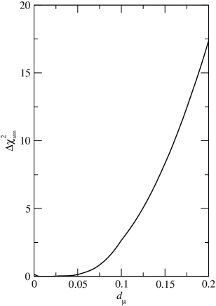
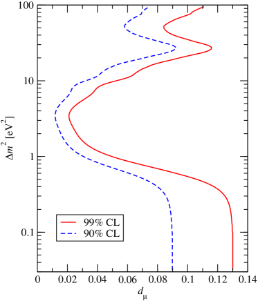
Figure 2: Left panel: $\Delta\chi^{2}_{\mathrm{atm}}$ as a function of $d_{\mu}$. Right panel: 90% and 99% CL upper bounds on $d_{\mu}$ by combining atmospheric neutrino data and the CDHS experiment.

In the left panel of Fig. 2 we show $\Delta\chi^{2}_{\mathrm{atm}}=\chi^{2}_{\mathrm{atm}}-(\chi^{2}_{\mathrm{atm}})_{\mathrm{min}}$ from the fit to atmospheric neutrino data as a function of the parameter $d_{\mu}$. For each value of $d_{\mu}$ the $\chi^{2}$ is minimized with respect to all other undisplayed parameters necessary to fit the atmospheric neutrino data. In the right panel of Fig. 2 we show the 90% and 99% CL bounds on $d_{\mu}$ obtained from a combination of all the atmospheric neutrino data with the $\nu_{\mu}$ disappearance experiment CDHS in a Bayesian framework.

In the lower part of this plot the constraint on $d_{\mu}$ comes from atmospheric neutrino data alone, as the CDHS bound disappears for $\Delta m^{2}\lesssim 0.3$ eV². Hence, atmospheric neutrino data leads to the bound

$$d_{\mu}\leq 0.090\,(0.13)\quad\mathrm{at}\quad 90\%\,(99\%)\,\mathrm{CL}\,.$$ (4)

Let us note that Fig. 2 and the bound given in Eq. (4) are valid also for the (2+2) spectra if the parameter $d_{\mu}$ is identified with $|K_{\mu 1}|^{2}+|K_{\mu 2}|^{2}$ and neutrino masses are labeled according to Fig. 1 (right).

4 An upper bound on $A_{\mu;e}$

In this section we discuss the upper bound on the LSND amplitude $A_{\mu;e}$ obtained by combining the data of the SBL experiments Bugey, CDHS, KARMEN and NOMAD, with those of the atmospheric neutrino experiments and the CHOOZ experiment. Here we focus mainly on the results of the extendend analysis, technical details can be found in Ref. [18].

To combine all the oscillation data we use the likelihood function

$$\begin{split}\mathcal{L}_{\mathrm{osc}}(d_{e},d_{\mu},\Delta m^{2})&=\mathcal{L}_{\mathrm{Bugey}}(d_{e},\Delta m^{2})\,\mathcal{L}_{\mathrm{CDHS}}(d_{\mu},\Delta m^{2})\\ &\times\mathcal{L}_{\mathrm{KARMEN}}(d_{e}d_{\mu},\Delta m^{2})\,\mathcal{L}_{\mathrm{NOMAD}}(d_{e}d_{\mu},\Delta m^{2})\\ &\times\mathcal{L}_{\mathrm{atm}}(d_{\mu})\,\mathcal{L}_{\mathrm{CHOOZ}}(d_{e})\,.\end{split}$$ (5)

The likelihood functions $\mathcal{L}_{\mathrm{Bugey}}$, $\mathcal{L}_{\mathrm{CDHS}}$ and $\mathcal{L}_{\mathrm{KARMEN}}$ are described in Ref. [18] and $\mathcal{L}_{\mathrm{atm}}\propto\exp\left(-\frac{1}{2}\chi^{2}_{\mathrm{atm}}\right)$ [42]. To calculate $\mathcal{L}_{\mathrm{NOMAD}}$ we perform a re-analysis of the $\nu_{\mu}\to\nu_{e}$ oscillation search at NOMAD by using the data given in Ref. [23]. The result of the CHOOZ experiment is included via $\mathcal{L}_{\mathrm{CHOOZ}}$, which is obtained with the maximum likelihood method described also in Ref. [18].

For a fixed value of $\Delta m^{2}$ the likelihood function Eq. (5) is transformed into a probability distribution $p(d_{e},d_{\mu})$ by applying Bayes’ theorem (see for example Refs. [42, 43]) and assuming a flat prior in the physically allowed region $d_{e},d_{\mu}\geq 0$ and $d_{e}+d_{\mu}\leq 1$. Choosing a CL $\beta$, we find the corresponding upper bound $A^{0}_{\beta}$ on $A_{\mu;e}$ by the prescription

$$\int\limits_{4d_{e}d_{\mu}\leq A^{0}_{\beta}}\hskip-10.0pt\mathrm{d}d_{e}\,\mathrm{d}d_{\mu}\,p(d_{e},d_{\mu})=\beta\,.$$ (6)

The bounds at 95% and 99% CL are shown in Fig. 3 together with the regions allowed by LSND at 90% and 99% CL. We find that there is no overlap of the region allowed by our bound at 95% CL with the region allowed by LSND at 99% CL [18]. If we take our bound at 99% CL there are marginal overlaps with the 99% CL LSND allowed region at $\Delta m^{2}\sim 0.9$ and 2 eV², and a very marginal overlap region still exists around 6 eV². The overlap region found in Ref. [18] between 0.25 and 0.4 eV² is now excluded by our bound at 99% CL because of the inclusion of the full atmospheric neutrino data set.

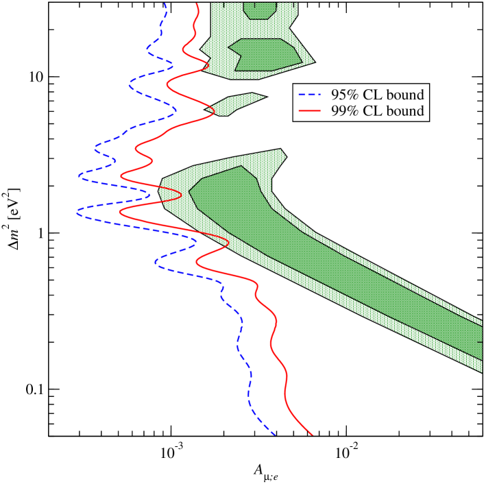
Figure 3: Upper bounds on the LSND amplitude $A_{\mu;e}$ at 95% and 99% CL. The shaded regions are the regions allowed by LSND at 90% and 99% CL [5].

For the alternative case of symmetric (2+2) spectra the bound on the LSND amplitude $A_{\mu;e}$ is dominated by the Bugey bound on $d_{e}$ and by the KARMEN bound on $A_{\mu;e}$. Hence, an improvement of the bound on $d_{\mu}$ by the inclusion of the full atmospheric neutrino data does not lead to a stronger bound on $A_{\mu;e}$ in this case so that the results of Ref. [18] apply. The conclusion is that (2+2) spectra are in good agreement with SBL data (see Fig. 2 of Ref. [18]). As shown in [35] they are also in agreement with the totality of solar and atmospheric neutrino data.

5 Implications of tritium $\beta$-decay

Experiments studying the electron spectrum $\mathrm{d}N/\mathrm{d}E_{e}$ from tritium $\beta$-decay can obtain information on the quantity $m_{\beta}^{2}$ determined by the relation

$$\frac{\mathrm{d}N}{\mathrm{d}E_{e}}\propto\sqrt{(E_{e}-E_{0})^{2}-m_{\beta}^{2}}\,,$$ (7)

where $E_{e}$ is the energy of the electron and $E_{0}$ is the total decay energy. The latest result obtained by the Troitsk experiment is [25]

$$m_{\beta}^{2}=-1.0\pm 3.0\pm 2.1\,\mathrm{eV}^{2}\,,\qquad m_{\beta}<2.5\,\mathrm{eV}\,.$$ (8)

The Mainz collaboration recently presented two values, obtained from different analyses of their data [26]:

$$m_{\beta}^{2} =+0.6\pm 2.8\pm 2.1\,\mathrm{eV}^{2}\,,\qquad m_{\beta}<2.8\,\mathrm{eV}\,,$$ (9)

$$m_{\beta}^{2} =-1.6\pm 2.5\pm 2.1\,\mathrm{eV}^{2}\,,\qquad m_{\beta}<2.2\,\mathrm{eV}\,.$$ (10)

In Eqs. (8)–(10) the upper bounds are at 95% CL.

Let us now consider the implications of these measurements for the (3+1)A and (3+1)B neutrino mass schemes (see Fig. 1). In the presence of neutrino mixing relation (7) has to be modified to (see e.g. [46])

$$\frac{\mathrm{d}N}{\mathrm{d}E_{e}}\propto\sum_{i=1}^{4}|K_{ei}|^{2}\,\sqrt{(E_{e}-E_{0})^{2}-m_{i}^{2}}\,\Theta(E_{0}-E_{e}-m_{i})\,.$$ (11)

In view of the very strong constraint on $d_{e}$ from Bugey we can safely neglect the contribution from $|K_{e4}|^{2}$ to the sum in Eq. (11). Further we take into account that mass splittings implied by solar and atmospheric neutrino data cannot be resolved in tritium decay experiments [46]. Hence, in spectra (3+1)A the value $m_{\beta}$ is given by the lowest neutrino mass and is independent of $\Delta m^{2}$ to a good approximation. Therefore, we do not include any information from tritium $\beta$-decay in this case. However, for spectra of the type (3+1)B one obtains [47] $m_{\beta}^{2}\approx m_{4}^{2}+\Delta m^{2}$. We include this result in our statistical analysis by using the likelihood function

$$\mathcal{L}_{\beta}(\Delta m^{2})\propto\begin{cases}\mathrm{const}&\text{for (3+1)A}\\ \exp\left[-\frac{1}{2}\sum\limits_{i}\left(\frac{(m_{\beta}^{2})_{i}-{\Delta m^{2}}-{m^{2}_{4}}}{\sigma_{i}}\right)^{2}\right]&\text{for (3+1)B}\end{cases}$$ (12)

where the sum is over the three experimental values of $m_{\beta}^{2}$ given in Eqs. (8)–(10) and $\sigma_{i}$ is the corresponding error (statistical and systematic errors added in quadrature). For fixed values of $m_{4}$ we perform now an analysis with the two parameters $A_{\mu;e}$ and $\Delta m^{2}$, in contrast to Sec. 4, where the analysis is performed only with the parameter $A_{\mu;e}$ for each value of $\Delta m^{2}$.

As a first step the total likelihood function obtained from Eqs. (5) and (12)

$$\mathcal{L}_{\mathrm{tot}}(d_{e},d_{\mu},\Delta m^{2})=\mathcal{L}_{\beta}(\Delta m^{2})\,\mathcal{L}_{\mathrm{osc}}(d_{e},d_{\mu},\Delta m^{2})$$ (13)

is transformed into a probability distribution $p(d_{e},d_{\mu},\log\Delta m^{2})$ by using Bayes’ theorem. We assume a flat prior distribution for $d_{e}$ and $d_{\mu}$ in the physical region and a flat prior distribution for $\log\Delta m^{2}$. This ensures that we introduce no bias concerning the order of magnitude of $\Delta m^{2}$, a priori all scales are equally probable. Then we perform a transformation of the variables $d_{e}$ and $d_{\mu}$ to

$$A_{\mu;e}=4\,d_{e}d_{\mu}\,,\quad t=\frac{1}{8}\ln\frac{d_{\mu}}{d_{e}}$$ (14)

and integrate over the variable $t$ to obtain the probability distribution for the variables we are interested in: $p(A_{\mu;e},\log\Delta m^{2})$. We calculate an allowed region at the 100$\beta$% CL by demanding

$$\int\mathrm{d}A_{\mu;e}\mathrm{d}(\log\Delta m^{2})\,p(A_{\mu;e},\log\Delta m^{2})=\beta\,.$$ (15)

The boundary in the $(A_{\mu;e},\Delta m^{2})$ plane is determined such that the value of $p(A_{\mu;e},\log\Delta m^{2})$ along this line is constant.

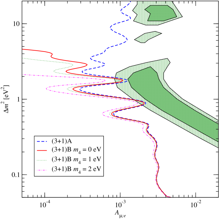
Figure 4: Allowed regions at 99% CL in the $(A_{\mu;e},\Delta m^{2})$ plane for spectra of the types (3+1)A and (3+1)B including tritium $\beta$-decay. In case of (3+1)B we show the regions for values of the lightest neutrino mass $m_{4}=0$, 1 and 2 eV. The shaded regions are the regions allowed by LSND at 90% and 99% CL [5].

In Fig. 4 we show the allowed regions at 99% CL for spectra of the types (3+1). In the case of (3+1)B we show the regions for $m_{4}=0$, 1 and 2 eV. As we do not know the true value of $m_{4}$ the curve corresponding to vanishing $m_{4}$ is the most conservative one. In this case tritium $\beta$-decay rules out values of $\Delta m^{2}\gtrsim 5$ eV². In both cases (3+1)A and (3+1)B ($m_{4}=0$) only two marginal overlaps with the 99%CL LSND allowed region survive at $\Delta m^{2}\sim 0.9$ and $2$ eV². For (3+1)B with $m_{4}=2$ eV the overlap with LSND disappears.

The following remarks are in order:

1. To normalize the probability distribution $p(A_{\mu;e},\log\Delta m^{2})$ one has to choose a lower integration bound for $\log\Delta m^{2}$ as $p(A_{\mu;e},\log\Delta m^{2})$ does not vanish for $\log\Delta m^{2}\to-\infty$. The allowed regions in Fig. 4 depend somewhat on this lower bound. However, if one chooses the lower bound sufficiently small ($\log\Delta m^{2}\lesssim-3$) the allowed regions become independent of it. In the case of the spectra (3+1)A the allowed region depends also on the upper integration bound for $\log\Delta m^{2}$. However, again the dependence disappears, if this bound is chosen large enough ($\log\Delta m^{2}\gtrsim 2$).

2. Note that the statistical meaning of the bounds in Figs. 3 and 4 is different. The method applied in Sec. 4 to produce Fig. 3 allows to place an upper bound on $A_{\mu;e}$ for a given value of $\Delta m^{2}$ at a certain CL, whereas the meaning of the 99% CL bounds shown in Fig. 4 is the following: the true values of $A_{\mu;e}$ and of $\Delta m^{2}$ are expected to lie at the left of the curves shown in the figure with probability 0.99. This explains the small differences between the curve for the (3+1)A spectra in Fig. 4 and the 99% CL curve in Fig. 3. However, the general agreement of both methods renders confidence to our analysis.

3. In our analysis we take into account only the shape of the likelihood as a function of $\Delta m^{2}$ for fixed values of $m_{4}$; for each given value of $m_{4}$ the likelihood function is normalized to 1. However, because of the relation $m_{\beta}\approx\sqrt{m_{4}^{2}+\Delta m^{2}}$ in scheme (3+1)B there are additional strong constraints on the allowed values of $\Delta m^{2}$ and $m_{4}$ from the upper bounds on $m_{\beta}$ given in Eqs. (8)–(10).

Finally, we note that the non-observation of neutrinoless double $\beta$-decay may also place important restrictions on (3+1)B spectra [47], where the electron neutrino has a substantial component along the heaviest neutrinos. However, this will be very model dependent as the resulting bounds are subject to possible destructive interference due to cancellations among different neutrinos [14, 48].

6 Conclusions

We have extended the analysis of neutrino oscillation data in the framework of (3+1) neutrino mass spectra performed in Ref. [18]. In addition to the full data from the short-baseline experiments Bugey [19], CDHS [20], KARMEN [21] and the result of the long-baseline reactor experiment CHOOZ [22], we have included also the full and updated data set of atmospheric neutrino experiments, the data from the $\nu_{\mu}\to\nu_{e}$ oscillation search in NOMAD [23] and tritium $\beta$-decay data [25, 26]. We have shown that the interpretation of the LSND anomaly within such schemes is severely disfavored by the combined data, in contrast to the case of the theoretically preferred (2+2) schemes. Since the details of the solar data do not play an important role in our (3+1) analysis, the most recent SNO results [24] will not affect the conclusions derived in our paper, nor contribute to enhance the bounds we have derived. Our present results put an additional challenge on some recent attempts to revive (3+1) schemes [12, 16, 17].

References

- [1] B.T. Cleveland et al., Astrophys. J. 496 (1998) 505; K.S. Hirata et al., Kamiokande Coll., Phys. Rev. Lett. 77 (1996) 1683; W. Hampel et al., GALLEX Coll., Phys. Lett. B 447 (1999) 127; D.N. Abdurashitov et al., SAGE Coll., Phys. Rev. Lett. 83 (1999) 4686; Y. Fukuda et al., Super-Kamiokande Coll., Phys. Rev. Lett. 81 (1998) 1158.
- [2] Y. Fukuda et al., Super-Kamiokande Coll., Phys. Rev. Lett. 81 (1998) 1562.
- [3] Y. Fukuda et al., Kamiokande Coll., Phys. Lett. B 335 (1994) 237; R. Becker-Szendy et al., IMB Coll., Nucl. Phys. B (Proc. Suppl.) 38 (1995) 331; W.W.M. Allison et al., Soudan Coll., Phys. Lett. B 449 (1999) 137; M. Ambrosio et al., MACRO Coll., Phys. Lett. B 434 (1998) 451.
- [4] C. Athanassopoulos et al., LSND Collaboration, Phys. Rev. Lett. 77 (1996) 3082; ibid 81 (1998) 1774.
- [5] G. Mills, LSND Coll., Talk given at Neutrino 2000, 15–21 June 2000, Sudbury, Canada, transparencies available at http://nu2000.sno.laurentian.ca.
- [6] O. Miranda, et al Nucl. Phys. B 595 (2001) 360; J. Pulido and E. Akhmedov, Phys. Lett. B485 (2000) 178; M.M. Guzzo and H. Nunokawa, Astropart. Phys. 12 (1999) 8; J. Derkaoui and Y. Tayalati, Astropart. Phys. 14 (2001) 351.
- [7] J.T. Peltoniemi, D. Tommasini and J.W.F. Valle, Phys. Lett. B 298 (1993) 383; J.T. Peltoniemi and J.W.F. Valle, Nucl. Phys. B 406 (1993) 409.
- [8] D.O. Caldwell and R.N. Mohapatra, Phys. Rev. D 48 (1993) 3259.
- [9] E. Ma and P. Roy, Phys. Rev. D 52 (1995) R4780; E.J. Chun et al., Phys. Lett. B 357 (1995) 608; J.J. Gomez-Cadenas and M.C. Gonzalez-Garcia, Z. Phys. C 71 (1996) 443; E. Ma, Mod. Phys. Lett. A 11 (1996) 1893; S. Goswami, Phys. Rev. D 55 (1997) 2931.
- [10] Q.Y. Liu and A. Smirnov, Nucl. Phys. B 524 505; V. Barger, K. Whisnant and T. Weiler, Phys. Lett. B 427 (1998) 97; S. Gibbons, R.N. Mohapatra, S. Nandi and A. Raichoudhuri, Phys. Lett. B 430 (1998) 296; Nucl. Phys. B 524 (1998) 505; E.J. Chun, A. Joshipura and A. Smirnov, in Elementary Particle Physics: Present and Future (World Scientific, 1996), ISBN 981-02-2554-7; P. Langacker, Phys. Rev. D 58 (1998) 093017; M. Bando and K. Yoshioka, Prog. Theor. Phys. 100 (1998) 1239; W. Grimus, R. Pfeiffer and T. Schwetz, Eur. Phys. J. C 13 (2000) 125; F. Borzumati, K. Hamaguchi and T. Yanagida, Phys. Lett. B 497 (2001) 259.
- [11] M. Hirsch and J.W.F. Valle, Phys. Lett. B 495 (2000) 121.
- [12] V. Barger et al., Phys. Lett. B 489 (2000) 345.
- [13] A. Ioannisian and J.W.F. Valle, Phys. Rev. D 63 (2001) 073002 [hep-ph/9911349].
- [14] J. W. F. Valle, Phys. Rev. D 27 (1983) 1672.
- [15] L. Wolfenstein, Nucl. Phys. B 186 (1981) 147.
- [16] C. Giunti and M. Laveder, JHEP 0102 (2001) 001.
- [17] O.L.G. Peres and A.Yu. Smirnov, Nucl. Phys. B 599 (2001) 3.
- [18] W. Grimus and T. Schwetz, Eur. Phys. J. C 20 (2001) 1.
- [19] B. Achkar et al., Bugey Coll., Nucl. Phys. B 434 (1995) 503.
- [20] F. Dydak et al., CDHS Coll., Phys. Lett. B 134 (1984) 281.
- [21] K. Eitel, KARMEN Coll., Talk given at Neutrino 2000, 15–21 June 2000, Sudbury, Canada, hep-ex/0008002
- [22] M. Apollonio et al., CHOOZ Coll., Phys. Lett. B 466 (1999) 415.
- [23] M. Mezzetto, NOMAD Coll., Nucl. Phys. B (Proc. Suppl.) 70 (1999) 214; L. Camilleri, NOMAD Coll., A Status Report (1999), http://nomadinfo.cern.ch/Public/PUBLICATIONS/.
- [24] Q.R. Ahmad et al., SNO Coll., nucl-ex/0106015.
- [25] V.M. Lobashev, Talk given at Neutrino 2000, 15–21 June 2000, Sudbury, Canada, Nucl. Phys. B (Proc. Suppl.) 91 (2001) 280.
- [26] C. Weinheimer, Talk given at Neutrino 2000, 15–21 June 2000, Sudbury, Canada, J. Bonn et al., Nucl. Phys. B (Proc. Suppl.) 91 (2001) 273.
- [27] S.M. Bilkenky, C. Giunti and W. Grimus, in Proceedings of Neutrino ’96, Helsinki, Finland, 13–19 June 1996, p. 174, edited by K. Enqvist, K. Huitu and J. Maalampi (World Scientific, Singapore 1997); S.M. Bilenky, C. Giunti and W. Grimus, Eur. Phys. J. C 1 (1998) 247.
- [28] N. Okada and O. Yasuda, Int. J. Mod. Phys. A 12 (1997) 3669.
- [29] S.M. Bilenky, C. Giunti, W. Grimus and T. Schwetz, Phys. Rev. D 60 (199) 073007.
- [30] V. Barger, S. Pakvasa, T.J. Weiler and K. Whisnant, Phys. Rev. D 58 (1998) 093016.
- [31] N. Fornengo, M.C. Gonzalez-Garcia and J.W.F. Valle, Nucl. Phys. B 580 (2000) 58; M.C. Gonzalez-Garcia, H. Nunokawa, O.L. Peres and J.W.F. Valle, Nucl. Phys. B 543 (1999) 3 and references therein.
- [32] Super-Kamiokande presentations in winter conferences: C. McGrew in Neutrino Telescopes 2001, Venice, Italy, March 2001, to appear; T. Toshito in Moriond 2001, Les Arcs, France, March 2001, to appear.
- [33] V. Barger et al., hep-ph/0106207; G.L. Fogli et al., hep-ph/0106247; J.N. Bahcall et al., hep-ph/0106258; A. Bandyopadhyay et al., hep-ph/0106264; P. Creminelli et al., hep-ph/0102234.
- [34] M.C. Gonzalez-Garcia, P.C. deHolanda, C. Peña-Garay and J.W.F. Valle, Nucl. Phys. B 573 (2000) 3 and references therein.
- [35] M.C. Gonzalez-Garcia, M. Maltoni and C. Peña-Garay, hep-ph/0105269, to appear in Phys. Rev. D.
- [36] J. Schechter and J.W.F. Valle, Phys. Rev. D 22 (1980) 2227; ibid 23 (1981) 1666.
- [37] J. Schechter and J.W.F. Valle, Phys. Rev. D 21 (1980) 309.
- [38] K.A. Olive and D. Thomas, Astropart. Phys. 11 (1999) 403; E. Lisi, S. Sarkar and F.L. Villante, Phys. Rev. D 59 (1999) 123520 and references therein.
- [39] S.M. Bilenky, C. Giunti, W. Grimus and T. Schwetz, Astropart. Phys. 11 (1999) 413.
- [40] M. Spurio et al., MACRO Coll., hep-ex/0101019; B. Barish, MACRO Coll., Talk given at Neutrino 2000, 15–21 June 2000, Sudbury, Canada.
- [41] M.C. Gonzalez-Garcia, M. Maltoni, C. Peña-Garay and J.W.F. Valle, Phys. Rev. D 63 (2001) 033005.
- [42] D.E. Groom et al., Particle Data Group, Eur. Phys. J. C 15 (2000) 1.
- [43] G. Cowan, Statistical Data Analysis (Oxford University Press, New York 1998); B.P. Roe, Probability and Statistics in Experimental Physics (Springer, New York 1992); G. Cowan, in Present and Future CP Measurements, p. 98, hep-ph/0102159.
- [44] L. Borodovsky et al., Phys. Rev. Lett. 68 (1992) 274.
- [45] A. Romosan et al., Phys. Rev. Lett. 78 (1997) 2912.
- [46] Y. Farzan, O.L.G. Peres and A.Yu. Smirnov, hep-ph/0105105.
- [47] S.M. Bilenky, S. Pascoli and S.T. Petcov, hep-ph/0104218.
- [48] L. Wolfenstein, Phys. Lett. B 107 (1981) 77.