Probing colored glass
via $q\bar{q}$ photoproduction

Abstract

In this paper, we calculate the cross-section for the photoproduction of quark-antiquark pairs in the peripheral collision of ultra-relativistic nuclei, by treating the color field of the nuclei within the Color Glass Condensate model. We find that this cross-section is sensitive to the saturation scale $Q_{s}^{2}$ that characterizes the model. In particular, the transverse momentum spectrum of the produced pairs could be used to measure the properties of the color glass condensate.

BNL-NT-01/15

1 Introduction

In recent years, there has been a lot of interest in the description of the distribution of partons inside a hadron or nucleus (see [1, 2] for a pedagogical introduction). An outstanding issue is the problem of the saturation of the parton distributions at very small values of the momentum fraction $x$ [3, 4, 5]. Indeed, the BFKL [6, 7, 8] equation predicts an uninterrupted rise of this distribution as $x$ becomes smaller and smaller. However, this is not compatible with unitarity, but rather an artifact of the linear nature of this equation: in other words, the BFKL equation becomes inadequate when the phase-space density approaches $1/\alpha_{s}$ [3, 9, 10]. This is an effect of the nonlinearity of QCD, and happens even at small coupling.

Many of the recent investigations are based on a model introduced by McLerran and Venugopalan [11, 12, 13], which describes the small $x$ gluons inside a fast moving nucleus by a classical color field. This approximation is justified by the large occupation number of the soft gluon modes. In this model, the classical Yang-Mills equation satisfied by the classical color field is driven by the current induced by the hard partons. The distribution of hard color sources inside the nucleus is described by a functional density which is taken to be Gaussian in the simplest forms of this model. This physical picture describes what can be called a “Color Glass Condensate”. The classical version of this model depends only on one parameter, called “saturation scale” and denoted $Q_{s}$, defined as the transverse momentum scale below which saturation effects start being important. This scale increases with energy and with the size of the nucleus [1, 9, 14]. Therefore, at energies high enough so that $Q_{s}\gg\Lambda_{{}_{QCD}}$, the coupling constant at the saturation scale is a small parameter and a perturbative approach can be considered. In that case, “perturbative” means that one can work at lowest order in $\alpha_{s}$, but all orders in the large classical color field must be kept in principle.

Many theoretical improvements have dealt with the quantum corrections to this model. When going to smaller values of $x$, one must integrate out the modes comprised between the new scale and the former scale [9]. Therefore, the functional density describing the distribution of hard sources has been found to obey a functional renormalization group equation [15, 16] that pilots its variations when one moves the separation scale between the hard and soft scale. Developments along those lines can be found in [17, 18, 19, 20, 21, 22, 23]. A particularly simple and suggestive form of this equation has been found recently [24, 25], as well as approximate solutions [26].

On the phenomenological side, this model has been used in order to study the fermionic degrees of freedom at small $x$ and compute structure functions like $F_{2}$ [27]. It has also been used to study the production of gluons in the collision of two color sources by several groups of authors. [28, 29] calculated the production of gluons at lowest order in the density of soft gluons. Then, Krasnitz and Venugopalan [30, 31] attacked the problem of the gluon production to all orders, by solving the classical Yang-Mills equation on a 2-dimensional lattice for an SU(2) gauge theory. Recently, this problem has been solved analytically for the case of $pA$ collisions [32], for which the gluon density for one source is much smaller than that of the second source. However, all these studies deal with the central collision of two objects (AA, pA), and the computed number of gluons cannot be observed directly. Instead, several layers of complex processes are to be taken into account between the stage where gluons are initially produced, and the stage where hadrons are observed in a detector (in particular, the hydrodynamical evolution, and the freeze-out of the system).

For this reason, it would be useful to consider a process which is sensitive to the distinctive features of the color glass condensate model, and yet can be observed in peripheral collisions. The second condition implies that such a process involves electromagnetic interactions in some way, because they are long-ranged. Since this process should also be sensitive to the gluon density, it has to involve quarks, which couple both to photons and gluons. Therefore, the simplest such process is the photoproduction of $q\bar{q}$ pairs, which has already been considered as an interesting probe for the gluon distribution [33, 34]. The simplest diagram for this process has been represented in figure 1.

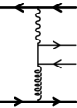
Figure 1: Prototype of the diagrams contributing to the photoproduction of a $q\bar{q}$ pair in $AA$ collisions.

In this paper, we calculate this process for the peripheral collision of two large ultra-relativistic nuclei. We treat the electromagnetic interaction to lowest order (or, equivalently, to the leading logarithmic approximation), and the interactions with the color field of the nucleus to all orders in the classical color field. We find that this process can indeed take place at large impact parameters, and is very sensitive to the features of the gluon distribution, for quarks whose mass is close to the saturation scale. We predict that the transverse momentum spectrum $d\sigma_{{}_{T}}/dydk_{\perp}$ of the produced pairs has a maximum for a momentum close to $Q_{s}$, which could therefore be used as a way to measure the saturation scale.

The structure of this paper is as follows. In section 2, we outline briefly the main aspects of the color glass condensate model. In particular, we recall how the use of the covariant gauge can simplify the description of the system at the classical level.

In section 3, we detail the main steps of the calculation of the cross-section for the photoproduction of $q\bar{q}$ pairs. In particular, we explain how this quantity relates to Green’s functions evaluated in the classical field, how one can calculate the retarded quark propagator in this background field, and the impact parameter dependence of the average multiplicity.

Section 4 explains how the transverse momentum spectrum of the produced pairs can be used as a probe of the color glass condensate, and section 5 deals with the integrated cross-section.

Finally, section 6 is devoted to concluding remarks.

2 The color glass condensate

A few years ago, it was suggested that the color field of a strongly boosted nucleus can be described as a classical color field [11, 12, 13], thanks to the fact that the small $x$ gluonic modes have a very large occupation number.

The classical field $A^{\mu}$ describing the soft modes satisfies a classical Yang-Mills equation:

$$\left[D_{\mu},F^{\mu\nu}\right]=gJ^{\nu}\;,$$ (1)

driven by a source $J^{\nu}$ generated by the hard modes. Note that this current lives in the adjoint representation of $SU(N_{c})$: $J^{\nu}\equiv J^{\nu}_{a}T^{a}$. For a nucleus moving at very high velocity in the positive $z$ direction, this source has the Lorentz structure $J^{\mu}=\delta^{\mu+}J^{+}$. Since the current $J^{\mu}$ is covariantly conserved, we have:

$$\left[D_{\mu},J^{\mu}\right]=0\;,$$ (3)

which requires

$$J^{+}(x^{+},x^{-},{\tenimbf x}_{\perp})=W(x^{+},x^{-},{\tenimbf x}_{\perp})\rho(x^{-},{\tenimbf x}_{\perp})W^{\dagger}(x^{+},x^{-},{\tenimbf x}_{\perp})\;,$$ (4)

with

$$\rho(x^{-},{\tenimbf x}_{\perp})\equiv J^{+}(x^{+}_{0},x^{-},{\tenimbf x}_{\perp})\;,$$

$$W(x^{+},x^{-},{\tenimbf x}_{\perp})\equiv{\rm T}\exp\left\{ig\int_{x^{+}_{0}}^{x^{+}}dz^{+}\,A^{-}(z^{+},x^{-},{\tenimbf x}_{\perp})\right\}\;.$$ (5)

Therefore, unlike in QED, the color source $J^{+}$ cannot be fixed independently of the field $A^{\mu}$ itself.

However, it is possible to simplify the problem by using the light-cone gauge defined by $A^{+}=0$, and by assuming that the physics is invariant under translations along the $x^{+}$ axis ($\partial^{-}=0$) because this is the direction of the nucleus trajectory. Under those assumptions, one can find solutions of the Yang-Mills equation for which $A^{-}=0$ (and hence $W=1$). More explicitly, the remaining Yang-Mills equations become

$$\left[D_{i},F^{ij}\right]=0\;,$$

$$\left[D_{i},\partial^{+}A^{i}\right]=-gJ^{+}\;.$$ (6)

The first of these equations indicates that the transverse components are a pure gauge field. Therefore, there is a unitary matrix $V$ such that:

$$A^{i}={i\over g}\,V^{\dagger}(x^{-},{\tenimbf x}_{\perp})\partial^{i}V(x^{-},{\tenimbf x}_{\perp})\;.$$ (7)

By plugging this $A^{i}$ into the second equation, one obtains an equation for $V$ in terms of the source $\rho$. It is however simpler to perform a gauge transformation generated by this $V$:

$$A^{\mu}\to\widetilde{A}^{\mu}\equiv{i\over g}\,V\partial^{\mu}V^{\dagger}+VA^{\mu}V^{\dagger}\;,$$ (8)

which leads to

$$\widetilde{A}^{-}=0\;,$$

$$\widetilde{A}^{i}=0\;,$$

$$\widetilde{A}^{+}={i\over g}\,V\partial^{+}V^{\dagger}\;,$$ (9)

and to the Yang-Mills equation

$$-\nabla_{\perp}^{2}\widetilde{A}^{+}=g\widetilde{\rho}\;,$$ (10)

where $\widetilde{\rho}\equiv V\rho V^{\dagger}$ is the source in the new gauge. This equation has the simple structure of a 2-dimensional Poisson equation with a source $\widetilde{\rho}$, but remains very difficult to solve in terms of the light-cone gauge source $\rho$. However, for reasons that will become apparent later, it is sufficient to express $V$ in terms of the covariant gauge source $\widetilde{\rho}$:

$$V(x^{-},{\tenimbf x}_{\perp})={\rm T}\exp\left\{-ig^{2}\int_{-\infty}^{x^{-}}dz^{-}\,{1\over{\nabla_{\perp}^{2}}}\widetilde{\rho}_{a}(z^{-},{\tenimbf x}_{\perp})T^{a}\right\}\;.$$ (11)

Having a formal solution of the classical Yang-Mills equation for a given distribution $\widetilde{\rho}$ of the hard color sources, the method to use this model is the following. One first expresses the observable of interest in terms of the classical color field, or equivalently in terms of the covariant gauge source $\widetilde{\rho}$: ${\cal O}[\widetilde{\rho}]$. Then one must perform an ensemble average over the set of sources $\widetilde{\rho}$. The observed value of this observable is therefore

$$\left<{\cal O}\right>\equiv\int[d\widetilde{\rho}]w[\widetilde{\rho}]{\cal O}[\widetilde{\rho}]\;.$$ (12)

A simple ansatz for the distribution of color sources $w[\widetilde{\rho}]$ is to take a Gaussian distribution:

$$w[\widetilde{\rho}]\equiv\exp\left\{-\!\!\int dx^{-}d^{2}{\tenimbf x}_{\perp}{{\widetilde{\rho}_{a}(x^{-},{\tenimbf x}_{\perp})\widetilde{\rho}^{a}(x^{-},{\tenimbf x}_{\perp})}\over{2\mu^{2}(x^{-})}}\right\}\;.$$ (13)

In the above formula, $\mu^{2}(x^{-})dx^{-}$ has the interpretation of a density of hard color sources per unit of transverse area, in the slice between $x^{-}$ and $x^{-}+dx^{-}$. For a very ultra-relativistic nucleus, this function is strongly peaked around $x^{-}=0$. At this stage, it is easy to justify the use of either the light-cone gauge source $\rho$ or the covariant gauge source $\widetilde{\rho}$ in order to express observables. Indeed, the weight $w[\widetilde{\rho}]$ is invariant under the gauge transformation of the source, as is the measure $[d\widetilde{\rho}]$. The saturation scale $Q_{s}^{2}$ is related to the integral of $\mu^{2}(x^{-})$ over $x^{-}$ (see Eq. (70) in the appendix A for the definition). Its value is expected to be of the order of $1$GeV at RHIC and $2-3$GeV at LHC.

With such a weight, averages of products of sources $\widetilde{\rho}$ can all be expressed in terms of the average of the product of two of them

$$\left<\widetilde{\rho}_{a}(x^{-},{\tenimbf x}_{\perp})\widetilde{\rho}_{b}(y^{-},{\tenimbf y}_{\perp})\right>=\delta_{ab}\mu^{2}(x^{-})\delta(x^{-}-y^{-})\delta({\tenimbf x}_{\perp}-{\tenimbf y}_{\perp})\;,$$ (14)

thanks to Wick’s theorem. More precisely, the average of the product of an even number of $\widetilde{\rho}$’s is obtained by performing the sum over all the possible pairings of two $\widetilde{\rho}$’s, and the average of the product of an odd number of $\widetilde{\rho}$’s is vanishing.

3 Calculation of $d\sigma_{{}_{T}}/dy$

3.1 Relation to Green’s functions in the classical field

Let us start by giving the connection between the average number of pairs produced per collision in terms of a fermionic correlator in the classical background field. For a given configuration of the hard color sources, one can use the formalism developed in [35] to express this quantity in terms of the retarded quark propagator. Using the same notations as in [35], we have

$$\overline{n}[\widetilde{\rho}]=\int{{d^{3}{\tenimbf q}}\over{(2\pi)^{3}2\omega_{\tenimbf q}}}\int{{d^{3}{\tenimbf p}}\over{(2\pi)^{3}2\omega_{\tenimbf p}}}\Big{|}\overline{u}({\tenimbf q}){\cal T}_{R}^{(\widetilde{\rho})}(q,-p)v({\tenimbf p})\Big{|}^{2}\;$$ (15)

for the average number of pairs produced in a collision at impact parameter ${\tenimbf b}$. In this formula, ${\cal T}_{R}^{(\widetilde{\rho})}$ denotes the interacting part of the retarded propagator of a quark in the classical field generated by the covariant gauge color source $\widetilde{\rho}$ and the electromagnetic current of the other nucleus. Note also that this quantity can be made differential with respect to the quark or the antiquark momentum by not integrating over the corresponding momentum. This will be useful in order to calculate the multiplicity per unit of rapidity.

Then, averaging over the configurations $\widetilde{\rho}$ of the hard color source, one obtains $\overline{n}$:

$$\overline{n}=\left<\overline{n}[\widetilde{\rho}]\right>=\int[d\widetilde{\rho}]\;w[\widetilde{\rho}]\;\overline{n}[\widetilde{\rho}]\;.$$ (16)

Note that $\overline{n}$ depends on the impact parameter ${\tenimbf b}$ of the collision. By integrating over impact parameter, one obtains the total cross-section.

3.2 Retarded quark propagator

In order to calculate $\overline{n}$, we need the retarded propagator of a quark moving in a classical field made of the electromagnetic field of one nucleus, and the color field of the other nucleus. In [35], we have shown that the retarded propagator becomes very simple in the ultra-relativistic limit. This result was derived for QED, but since the argument was based only on causality, it can be extended immediately to QCD. Therefore, we can write formally (convolution products are not written explicitly) for the scattering matrix ${\cal T}_{R}$:

$${\cal T}_{R}^{(\widetilde{\rho})}=T_{R}^{{}^{QCD}}+T_{R}^{{}^{QED}}+T_{R}^{{}^{QCD}}G_{R}^{0}T_{R}^{{}^{QED}}+T_{R}^{{}^{QED}}G_{R}^{0}T_{R}^{{}^{QCD}}\;,$$ (17)

where $T_{R}^{{}^{QED}}$ and $T_{R}^{{}^{QCD}}$ are the retarded scattering matrices of the quark in the electromagnetic field of the first nucleus and in the color field of the second nucleus respectively. $G_{R}^{0}$ is the free retarded propagator of a quark, which has the following expression in Fourier space:

$$G_{R}^{0}(p)\equiv i{{\raise 0.43057pt\hbox{$/$}\kern-6.30005pt\hbox{$p$}+m}\over{p^{2}-m^{2}+2p^{0}\epsilon}}\;.$$ (18)

Assuming that the nucleus acting via its electromagnetic field is moving along the negative $z$ axis, we have in the ultra-relativistic limit

$$T_{R}^{{}^{QED}}(q,p)=2\pi\delta(p^{+}-q^{+})\raise 0.43057pt\hbox{$/$}\kern-6.30005pt\hbox{$v$}_{-}\int d^{2}{\tenimbf x}_{\perp}\Big{[}e^{-ie\Lambda({\tenimbf x}_{\perp})}-1\Big{]}e^{i({\tenimbf q}_{\perp}-{\tenimbf p}_{\perp})\cdot{\tenimbf x}_{\perp}}\;,$$ (19)

where $\Lambda({\tenimbf x}_{\perp})$ is the 2-dimensional Coulomb potential of the first nucleus. Note that this potential can also be written as

$$\Lambda({\tenimbf x}_{\perp})=\int_{-\infty}^{+\infty}dz^{-}{1\over{\nabla_{\perp}^{2}}}\rho(z^{-},{\tenimbf z}_{\perp})\;,$$ (20)

where $\rho(z^{-},{\tenimbf z}_{\perp})$ is the electric charge density inside the nucleus.

Since the second nucleus is also ultra-relativistic, we can assume that the quark does not resolve the longitudinal structure of the color source. The only difference with QED in that respect is the $z^{-}$-ordering. If one uses the gauge defined by equations (9), then the problem of the propagation of a quark through a color glass condensate is formally similar to the QED case, and we can generalize equation (19) without difficulty:

$$T_{R}^{{}^{QCD}}(q,p)=2\pi\delta(p^{-}-q^{-})\raise 0.43057pt\hbox{$/$}\kern-6.30005pt\hbox{$v$}_{+}\int d^{2}{\tenimbf x}_{\perp}\Big{[}U({\tenimbf x}_{\perp})-1\Big{]}e^{i({\tenimbf q}_{\perp}-{\tenimbf p}_{\perp})\cdot{\tenimbf x}_{\perp}}\;,$$ (21)

with

$$U({\tenimbf x}_{\perp})\equiv{\rm T}\exp\left\{-ig^{2}\int_{-\infty}^{+\infty}dz^{-}{1\over{\nabla_{\perp}^{2}}}\widetilde{\rho}_{a}(z^{-},{\tenimbf x}_{\perp})t^{a}\right\}\;.$$ (22)

This formula also takes into account the fact that this nucleus is moving in the positive $z$ direction. The inverse Laplacian acting on the covariant gauge color source, integrated along the axis of the collision, is the analogue of the 2-dimensional Coulomb potential in QED (see Eq. (20)). Note also that the covariant gauge color source is now contracted with the generators of the fundamental representation. More details on the eikonal approximation in a color glass condensate can be found in [36].

For pair production, only the last two terms in Eq. (17) are relevant, because one cannot produce a $q\bar{q}$ pair on-shell by interacting with only one nucleus. After doing the integrals over the $+$ and $-$ components of the momentum transfer (made trivial by the delta functions), the relevant part of the retarded scattering matrix is:

$${\cal T}_{R}^{(\widetilde{\rho})}(q,-p)=-i\int{{d^{2}{\tenimbf k}_{\perp}}\over{(2\pi)^{2}}}F_{R}^{{}^{QCD}}({\tenimbf k}_{\perp})F_{R}^{{}^{QED}}({\tenimbf p}_{\perp}+{\tenimbf q}_{\perp}-{\tenimbf k}_{\perp})$$

$$\qquad\times\Big{\{}{{\raise 0.43057pt\hbox{$/$}\kern-6.30005pt\hbox{$v$}_{+}(\raise 0.43057pt\hbox{$/$}\kern-6.30005pt\hbox{$q$}-\raise 0.6458pt\hbox{$/$}\kern-5.29999pt\hbox{$k$}+m)\raise 0.43057pt\hbox{$/$}\kern-6.30005pt\hbox{$v$}_{-}}\over{2q^{-}p^{+}+({\tenimbf q}_{\perp}-{\tenimbf k}_{\perp})^{2}+m^{2}}}+{{\raise 0.43057pt\hbox{$/$}\kern-6.30005pt\hbox{$v$}_{-}(\raise 0.6458pt\hbox{$/$}\kern-5.29999pt\hbox{$k$}-\raise 0.43057pt\hbox{$/$}\kern-6.30005pt\hbox{$p$}+m)\raise 0.43057pt\hbox{$/$}\kern-6.30005pt\hbox{$v$}_{+}}\over{2q^{+}p^{-}+({\tenimbf p}_{\perp}-{\tenimbf k}_{\perp})^{2}+m^{2}}}\Big{\}}\;,$$ (23)

where we denote

$$F_{R}^{{}^{QCD}}({\tenimbf k}_{\perp})\equiv\int d^{2}{\tenimbf x}_{\perp}\left[U({\tenimbf x}_{\perp})-1\right]\,e^{i{\tenimbf k}_{\perp}\cdot{\tenimbf x}_{\perp}}\;,$$

$$F_{R}^{{}^{QED}}({\tenimbf k}_{\perp})\equiv\int d^{2}{\tenimbf x}_{\perp}\left[e^{-ie\Lambda({\tenimbf x}_{\perp})}-1\right]\,e^{i{\tenimbf k}_{\perp}\cdot{\tenimbf x}_{\perp}}\;.$$ (24)

In the following, it will prove convenient to factor out the impact parameter dependence contained in $F_{R}^{{}^{QED}}$ (we chose the origin of the transverse coordinates in such a way that the nucleus acting via its color field has its center at ${\tenimbf x}_{\perp}=0$, so that all the ${\tenimbf b}$ dependence goes into $F_{R}^{{}^{QED}}$), by writing

$$F_{R}^{{}^{QED}}({\tenimbf k}_{\perp})\equiv e^{i{\tenimbf k}_{\perp}\cdot{\tenimbf b}}f_{R}^{{}^{QED}}({\tenimbf k}_{\perp})\;.$$ (25)

Note that, at the Born level, we have

$$\left.f_{R}^{{}^{QED}}({\tenimbf k}_{\perp})\right|_{\rm Born}={{4\pi Z\alpha}\over{{\tenimbf k}_{\perp}^{2}}}\;,$$ (26)

where $\alpha=e^{2}/4\pi$ is the electromagnetic structure constant. The infrared sensitive denominator $1/{\tenimbf k}_{\perp}^{2}$ produces a large logarithm in the cross-section. Coulomb corrections beyond this Born term do not produce such a large logarithm [37, 38, 39], and will be discarded in this paper.

3.3 Expression of $\overline{n}$

Using the formula of Eq. (16), we can write

$$\overline{n}=\int{{d^{3}{\tenimbf p}}\over{(2\pi)^{3}2\omega_{\tenimbf p}}}{{d^{3}{\tenimbf q}}\over{(2\pi)^{3}2\omega_{\tenimbf q}}}\int{{d^{2}{\tenimbf k}_{\perp}}\over{(2\pi)^{2}}}\int{{d^{2}{\tenimbf l}_{\perp}}\over{(2\pi)^{2}}}{\rm Tr}_{c}\left<F_{R}^{{}^{QCD}}({\tenimbf k}_{\perp})F_{R}^{\dagger}{}^{{}^{QCD}}({\tenimbf l}_{\perp})\right>$$

$$\qquad\times F_{R}^{{}^{QED}}({\tenimbf p}_{\perp}+{\tenimbf q}_{\perp}-{\tenimbf k}_{\perp})F_{R}^{*}{}^{{}^{QED}}({\tenimbf p}_{\perp}+{\tenimbf q}_{\perp}-{\tenimbf l}_{\perp})$$

$$\qquad\times{\rm Tr}\,(M({\tenimbf p},{\tenimbf q}|{\tenimbf k}_{\perp})M^{*}({\tenimbf p},{\tenimbf q}|{\tenimbf l}_{\perp}))\;,$$ (27)

where ${\rm Tr}_{c}$ is a trace over color indices, ${\rm Tr}$ is the Dirac trace, and where we denote

$$M({\tenimbf p},{\tenimbf q}|{\tenimbf k}_{\perp})\equiv\overline{u}({\tenimbf q})\Big{\{}{{\raise 0.43057pt\hbox{$/$}\kern-6.30005pt\hbox{$v$}_{+}(\raise 0.43057pt\hbox{$/$}\kern-6.30005pt\hbox{$q$}-\raise 0.6458pt\hbox{$/$}\kern-5.29999pt\hbox{$k$}+m)\raise 0.43057pt\hbox{$/$}\kern-6.30005pt\hbox{$v$}_{-}}\over{2q^{-}p^{+}+({\tenimbf q}_{\perp}-{\tenimbf k}_{\perp})^{2}+m^{2}}}$$

$$\qquad\qquad\qquad\qquad\qquad+{{\raise 0.43057pt\hbox{$/$}\kern-6.30005pt\hbox{$v$}_{-}(\raise 0.6458pt\hbox{$/$}\kern-5.29999pt\hbox{$k$}-\raise 0.43057pt\hbox{$/$}\kern-6.30005pt\hbox{$p$}+m)\raise 0.43057pt\hbox{$/$}\kern-6.30005pt\hbox{$v$}_{+}}\over{2q^{+}p^{-}+({\tenimbf p}_{\perp}-{\tenimbf k}_{\perp})^{2}+m^{2}}}\Big{\}}v({\tenimbf p})\;.$$ (28)

Using the results of appendix A (see Eqs. (74) and (80)), we can rewrite this as

$$\overline{n}=N_{c}\int{{d^{3}{\tenimbf p}}\over{(2\pi)^{3}2\omega_{\tenimbf p}}}{{d^{3}{\tenimbf q}}\over{(2\pi)^{3}2\omega_{\tenimbf q}}}\int{{d^{2}{\tenimbf k}_{\perp}}\over{(2\pi)^{2}}}\int{{d^{2}{\tenimbf l}_{\perp}}\over{(2\pi)^{2}}}$$

$$\quad\times\int d^{2}{\tenimbf x}_{\perp}d^{2}{\tenimbf y}_{\perp}e^{i{\tenimbf k}_{\perp}\cdot{\tenimbf x}_{\perp}}e^{-i{\tenimbf l}_{\perp}\cdot{\tenimbf y}_{\perp}}{\cal P}({\tenimbf x}_{\perp}){\cal P}({\tenimbf y}_{\perp})\left[1+e^{-B_{2}({\tenimbf x}_{\perp}-{\tenimbf y}_{\perp})}-2e^{-B_{1}}\right]$$

$$\quad\times F_{R}^{{}^{QED}}({\tenimbf p}_{\perp}+{\tenimbf q}_{\perp}-{\tenimbf k}_{\perp})F_{R}^{*}{}^{{}^{QED}}({\tenimbf p}_{\perp}+{\tenimbf q}_{\perp}-{\tenimbf l}_{\perp})$$

$$\quad\times{\rm Tr}\,(M({\tenimbf p},{\tenimbf q}|{\tenimbf k}_{\perp})M^{*}({\tenimbf p},{\tenimbf q}|{\tenimbf l}_{\perp}))\;,$$ (29)

where the function ${\cal P}({\tenimbf x}_{\perp})$ describes the transverse profile of the nucleus (see the appendix A for more details on the effects of the nucleus finite size). For the terms in the square bracket which are independent of ${\tenimbf x}_{\perp}$ and ${\tenimbf y}_{\perp}$, the integral over those variables is trivial and just leads to the product $\widetilde{\cal P}({\tenimbf k}_{\perp})\widetilde{\cal P}({\tenimbf l}_{\perp})$ of the Fourier transforms of the functions ${\cal P}$. For a large nucleus, the Fourier transform $\widetilde{\cal P}({\tenimbf k}_{\perp})$ is very peaked around ${\tenimbf k}_{\perp}=0$, with a typical width of $1/R$, where $R$ is the radius of the nucleus. However, it is straightforward to check that

$$M({\tenimbf p},{\tenimbf q}|0)=M({\tenimbf p},{\tenimbf q}|{\tenimbf p}_{\perp}+{\tenimbf q}_{\perp})=0\;.$$ (30)

Moreover, the only scale controlling the amplitude $M({\tenimbf p},{\tenimbf q}|{\tenimbf k}_{\perp})$ is the mass $m$ of the produced quark, which means that it varies significantly only if ${\tenimbf k}_{\perp}$ changes by an amount comparable to $m$. Therefore, for heavy quarks such that $m\gg 1/R$, the function $M({\tenimbf p},{\tenimbf q}|{\tenimbf k}_{\perp})$ remains very close to zero over all the range over which $\widetilde{\cal P}({\tenimbf k}_{\perp})$ differs from zero. As a consequence, we can neglect the contribution of the terms independent of ${\tenimbf x}_{\perp}$ and ${\tenimbf y}_{\perp}$, and focus on the term proportional to $\exp(-B_{2}({\tenimbf x}_{\perp}-{\tenimbf y}_{\perp}))$.

Using now the approximation of Eq. (76) for the function $B_{2}({\tenimbf x}_{\perp}-{\tenimbf y}_{\perp})$, we see that this function becomes much larger than $1$ as soon as $|{\tenimbf x}_{\perp}-{\tenimbf y}_{\perp}|\gg Q_{s}^{-1}$. Since we have also $R\gg\Lambda_{{}_{QCD}}^{-1}\gg Q_{s}^{-1}$, it is reasonable to approximate the product ${\cal P}({\tenimbf x}_{\perp}){\cal P}({\tenimbf y}_{\perp})$ by a single factor ${\cal P}({\tenimbf x}_{\perp})$. The integral over ${\tenimbf x}_{\perp}$ and ${\tenimbf y}_{\perp}$ then becomes trivial and gives

$$\overline{n}=N_{c}\!\!\int{{d^{3}{\tenimbf p}}\over{(2\pi)^{3}2\omega_{\tenimbf p}}}{{d^{3}{\tenimbf q}}\over{(2\pi)^{3}2\omega_{\tenimbf q}}}\int\!{{d^{2}{\tenimbf k}_{\perp}}\over{(2\pi)^{2}}}\int\!{{d^{2}{\tenimbf l}_{\perp}}\over{(2\pi)^{2}}}e^{i({\tenimbf k}_{\perp}-{\tenimbf l}_{\perp})\cdot{\tenimbf b}}\widetilde{\cal P}({\tenimbf k}_{\perp}-{\tenimbf l}_{\perp})C({\tenimbf k}_{\perp})$$

$$\qquad\times f_{R}^{{}^{QED}}({\tenimbf p}_{\perp}+{\tenimbf q}_{\perp}-{\tenimbf k}_{\perp})f_{R}^{*}{}^{{}^{QED}}({\tenimbf p}_{\perp}+{\tenimbf q}_{\perp}-{\tenimbf l}_{\perp})$$

$$\qquad\times{\rm Tr}\,(M({\tenimbf p},{\tenimbf q}|{\tenimbf k}_{\perp})M^{*}({\tenimbf p},{\tenimbf q}|{\tenimbf l}_{\perp}))\;,$$ (31)

where we have defined

$$C({\tenimbf k}_{\perp})\equiv\int d^{2}{\tenimbf x}_{\perp}e^{i{\tenimbf k}_{\perp}\cdot{\tenimbf x}_{\perp}}e^{-B_{2}({\tenimbf x}_{\perp})}\;.$$ (32)

Using the Eqs. (68), (70), (71) and (74) of the appendix A, one can see that $C({\tenimbf k}_{\perp})$ is nothing but

$$C({\tenimbf k}_{\perp})=\int d^{2}{\tenimbf x}_{\perp}e^{i{\tenimbf k}_{\perp}\cdot{\tenimbf x}_{\perp}}\left<U(0)U^{\dagger}({\tenimbf x}_{\perp})\right>\;.$$ (33)

In other words, by assuming that the nucleus is large ($R\gg\Lambda_{{}_{QCD}}^{-1}$), we have been able to factorize the dependence on the nucleus size and recover the correlator $\left<U(0)U^{\dagger}({\tenimbf x}_{\perp})\right>$ associated to an hypothetical infinite nucleus.

3.4 Impact parameter dependence

From Eq. (31), one can determine the main features of the impact parameter dependence of the multiplicity $\overline{n}$. It is useful to recall that $M({\tenimbf p},{\tenimbf q}|{\tenimbf k}_{\perp})$ vanishes when ${\tenimbf p}_{\perp}+{\tenimbf q}_{\perp}={\tenimbf k}_{\perp}$. Moreover, since the typical transverse momentum ${\tenimbf p}_{\perp}+{\tenimbf q}_{\perp}-{\tenimbf k}_{\perp}$ has to be very small for coherent photons, compared to the other scales in $M({\tenimbf p},{\tenimbf q}|{\tenimbf k}_{\perp})$ which are controlled by the quark mass, on can use a Taylor expansion of this amplitude around the zero:

$$M({\tenimbf p},{\tenimbf q}|{\tenimbf k}_{\perp})\approx({\tenimbf p}_{\perp}+{\tenimbf q}_{\perp}-{\tenimbf k}_{\perp})\cdot{\tenimbf L}({\tenimbf p},{\tenimbf q})\;,$$ (34)

with

$${\tenimbf L}({\tenimbf p},{\tenimbf q})\equiv\overline{u}({\tenimbf q})\left\{{1\over{2(p^{+}+q^{+})}}\left({{\raise 0.43057pt\hbox{$/$}\kern-6.30005pt\hbox{$v$}_{+}{\boldsymbol{\gamma}}_{\perp}\raise 0.43057pt\hbox{$/$}\kern-6.30005pt\hbox{$v$}_{-}}\over{q^{-}}}-{{\raise 0.43057pt\hbox{$/$}\kern-6.30005pt\hbox{$v$}_{-}{\boldsymbol{\gamma}}_{\perp}\raise 0.43057pt\hbox{$/$}\kern-6.30005pt\hbox{$v$}_{+}}\over{p^{-}}}\right)\right.$$

$$\left.\qquad\qquad\qquad\qquad+{{\raise 0.43057pt\hbox{$/$}\kern-6.30005pt\hbox{$v$}_{-}}\over{(p^{+}+q^{+})^{2}}}\left({{{\tenimbf q}_{\perp}}\over{q^{-}}}-{{{\tenimbf p}_{\perp}}\over{p^{-}}}\right)\right\}v({\tenimbf p})\;.$$ (35)

In addition, the small transverse momentum of the photons allows one to write $C({\tenimbf k}_{\perp})\approx C({\tenimbf p}_{\perp}+{\tenimbf q}_{\perp})$. Therefore, one can see that the impact parameter dependence of $\overline{n}$ is completely controlled by the integral

$$I(b)\equiv\int{{d^{2}{\tenimbf m}_{\perp}}\over{(2\pi)^{2}}}{{d^{2}{\tenimbf n}_{\perp}}\over{(2\pi)^{2}}}\,e^{-i({\tenimbf m}_{\perp}-{\tenimbf n}_{\perp})\cdot{\tenimbf b}}\,\widetilde{\cal P}({\tenimbf m}_{\perp}-{\tenimbf n}_{\perp})\,{{{\tenimbf m}_{\perp}\cdot{\tenimbf L}({\tenimbf p},{\tenimbf q})}\over{{\tenimbf m}_{\perp}^{2}}}\,{{{\tenimbf n}_{\perp}\cdot{\tenimbf L}^{*}({\tenimbf p},{\tenimbf q})}\over{{\tenimbf n}_{\perp}^{2}}}\;,$$ (36)

where we have used the new variables ${\tenimbf m}_{\perp}\equiv{\tenimbf p}_{\perp}+{\tenimbf q}_{\perp}-{\tenimbf k}_{\perp}$ and ${\tenimbf n}_{\perp}\equiv{\tenimbf p}_{\perp}+{\tenimbf q}_{\perp}-{\tenimbf l}_{\perp}$. If the impact parameter is very large ($b\gg R$), then the momentum difference $|{\tenimbf m}_{\perp}-{\tenimbf n}_{\perp}|$ can at most be of order $1/b\ll 1/R$ because otherwise the exponential would average to zero. On such a small range, the function $\widetilde{\cal P}({\tenimbf m}_{\perp}-{\tenimbf n}_{\perp})$ can be replaced by $\widetilde{\cal P}(0)=\int d^{2}{\tenimbf x}_{\perp}{\cal P}({\tenimbf x}_{\perp})=\pi R^{2}$, and the integrals over ${\tenimbf m}_{\perp}$ and ${\tenimbf n}_{\perp}$ are trivial to perform. One obtains:

$$I(b)=\pi R^{2}{{{\tenimbf b}\cdot{\tenimbf L}({\tenimbf p},{\tenimbf q})}\over{2\pi b^{2}}}\,{{{\tenimbf b}\cdot{\tenimbf L}^{*}({\tenimbf p},{\tenimbf q})}\over{2\pi b^{2}}}\;.$$ (37)

Therefore, the multiplicity decreases like $1/b^{2}$ at large impact parameter. If taken seriously up to $b=+\infty$, this would lead to a logarithmic divergence in the cross-section after integration over ${\tenimbf b}$, as is well known in problems involving long ranged electromagnetic interactions. In reality the field does not keep its Weizsäcker-Williams form up to arbitrarily large transverse distances. Indeed, at the distance $b$ from the source, the field has a typical longitudinal extension of $b/\gamma$, where $\gamma$ is the Lorentz factor of the electromagnetic source. This width should be compared with the typical Compton wavelength of the particle being produced, i.e. $1/m$ in the present case, which leads to an upper cutoff $b=\gamma/m$ in the integral over impact parameter. This upper bound on $b$ is equivalent to the lower bound $m/\gamma$ on the transverse momentum of the photon. On the lower side, one must cutoff the integral at $b=2R$ in order to consider only peripheral collisions. Although these cutoffs are introduced by hand, this ansatz gives the leading logarithm correctly. This leading log approximation is valid if there is a large range between the scales $2R$ and $\gamma/m$. At smaller impact parameters, i.e. when $b$ is close to $2R$, the $1/b^{2}$ scaling law is modified by edge effects which are difficult to estimate analytically.

3.5 Evaluation of $d\sigma_{{}_{T}}/dy$

In order to obtain the leading logarithm of the cross-section for peripheral collisions (the ones that are phenomenologically interesting for photoproduction), we can use the formula Eq. (37) for all the range $2R\leq b\leq\gamma/m$. Noting that

$$\int d^{2}{\tenimbf b}\;{\tenimbf b}^{i}{\tenimbf b}^{j}f({\tenimbf b}^{2})={{\delta^{ij}}\over{2}}\int d^{2}{\tenimbf b}\;{\tenimbf b}^{2}f({\tenimbf b}^{2})\;,$$ (38)

we can write

$$\int d^{2}{\tenimbf b}\;{{{\tenimbf b}\cdot{\tenimbf L}}\over{b^{2}}}\,{{{\tenimbf b}\cdot{\tenimbf L}^{*}}\over{b^{2}}}={{{\tenimbf L}\cdot{\tenimbf L}^{*}}\over{2}}\;\int{{d^{2}{\tenimbf b}}\over{{\tenimbf b}^{2}}}\;.$$ (39)

Therefore, we have the following expression for the total cross-section for $q\bar{q}$ photoproduction in peripheral collisions:

$$\sigma_{{}_{T}}\equiv\int\limits_{2R}^{\gamma/m}d^{2}{\tenimbf b}\,\overline{n}=\pi R^{2}{2{N_{c}(Z\alpha)^{2}}}\int\limits_{2R}^{\gamma/m}{{d^{2}{\tenimbf b}}\over{{\tenimbf b}^{2}}}$$

$$\qquad\times\int{{d^{3}{\tenimbf p}}\over{(2\pi)^{3}2\omega_{\tenimbf p}}}{{d^{3}{\tenimbf q}}\over{(2\pi)^{3}2\omega_{\tenimbf q}}}C({\tenimbf p}_{\perp}+{\tenimbf q}_{\perp})\,{\rm Tr}\,\left(\left|{\tenimbf L}({\tenimbf p},{\tenimbf q})\right|^{2}\right)\;.$$ (40)

This is the formula we are going to use in the following. In Eq. (40), the factor which is the less well known analytically is the correlator $C({\tenimbf p}_{\perp}+{\tenimbf q}_{\perp})$. Therefore, in the evaluation of integrals, we are going to keep the variable ${\tenimbf p}_{\perp}+{\tenimbf q}_{\perp}$ (i.e. the total transverse momentum of the pair, or approximatively the momentum transfer between the color field and the $q\bar{q}$ pair) unintegrated until the end. At this stage, we will have the choice to use some analytic approximation of $C({\tenimbf p}_{\perp}+{\tenimbf q}_{\perp})$ or do the integral numerically. This approach also leaves open the possibility to consider other saturation models.

The first step is to perform the Dirac algebra, which leads to:

$${\rm Tr}\,\left(\left|{\tenimbf L}({\tenimbf p},{\tenimbf q})\right|^{2}\right)={4\over{(p^{-}q^{-}(p^{+}+q^{+}))^{2}}}$$

$$\qquad\qquad\times\left\{p^{-}q^{-}({\tenimbf p}_{\perp}+{\tenimbf q}_{\perp})^{2}-2{{(q^{+}q^{-}{\tenimbf p}_{\perp}+p^{+}p^{-}{\tenimbf q}_{\perp})^{2}}\over{(p^{+}+q^{+})^{2}}}\right\}\;.$$ (41)

One can check that the expression of Eq. (41) vanishes for ${\tenimbf p}_{\perp}+{\tenimbf q}_{\perp}=0$, i.e. when the momentum transfer from the color glass condensate is zero. By using the fact that the final state particles are on-shell, we can perform for free the integrals over $q^{+}$ and $p^{+}$. Then, the integral over $p^{-}$ is very easy because the dependence on this variable is rational. Noticing finally that $dq^{-}/q^{-}=2dy$, where $2y=\ln(q^{+}/q^{-})$ is the rapidity of the produced quark, it is very easy to obtain the differential cross-section with respect to the rapidity of the quark (or equivalently, of the antiquark):

$${{d\sigma_{{}_{T}}}\over{dy}}=\pi R^{2}{{8N_{c}(Z\alpha)^{2}}\over{\pi^{2}}}\int\limits_{2R}^{\gamma/m}{{d^{2}{\tenimbf b}}\over{{\tenimbf b}^{2}}}\int{{d^{2}{\tenimbf p}_{\perp}}\over{(2\pi)^{2}}}{{d^{2}{\tenimbf q}_{\perp}}\over{(2\pi)^{2}}}C({\tenimbf p}_{\perp}+{\tenimbf q}_{\perp})$$

$$\qquad\qquad\qquad\times\left\{{{({\tenimbf p}_{\perp}+{\tenimbf q}_{\perp})^{2}}\over{2\omega_{p}^{2}\omega_{q}^{2}}}-{1\over 6}\left[{{{\tenimbf p}_{\perp}}\over{\omega_{p}^{2}}}+{{{\tenimbf q}_{\perp}}\over{\omega_{q}^{2}}}\right]^{2}\right\}\;,$$ (42)

with $\omega_{p}^{2}\equiv{\tenimbf p}_{\perp}^{2}+m^{2}$ and $\omega_{q}^{2}\equiv{\tenimbf q}_{\perp}^{2}+m^{2}$. Let us take as one of the integration variables the total transverse momentum of the pair ${\tenimbf k}_{\perp}\equiv{\tenimbf p}_{\perp}+{\tenimbf q}_{\perp}$, and keep this variable unintegrated until the end. Then, it is easy to perform the integral over the vector ${\tenimbf q}_{\perp}$. An intermediate step is the integral over the angle $\theta$ between ${\tenimbf q}_{\perp}$ and ${\tenimbf k}_{\perp}$:

$$\int\limits_{0}^{2\pi}{{d\theta}\over{2\pi}}\left\{{{{\tenimbf k}_{\perp}^{2}}\over{2\omega_{k-q}^{2}\omega_{q}^{2}}}-{1\over 6}\left[{{{\tenimbf k}_{\perp}-{\tenimbf q}_{\perp}}\over{\omega_{k-q}^{2}}}+{{{\tenimbf q}_{\perp}}\over{\omega_{q}^{2}}}\right]^{2}\right\}$$

$$\qquad={{q_{\perp}^{2}+2k_{\perp}^{2}-m^{2}}\over{6(q_{\perp}^{2}+m^{2})\sqrt{(m^{2}+q_{\perp}^{2}+k_{\perp}^{2})^{2}-4q_{\perp}^{2}k_{\perp}^{2}}}}$$

$$\qquad-{{m^{2}(q_{\perp}^{2}+k_{\perp}^{2})+(q_{\perp}^{2}-k_{\perp}^{2})^{2}}\over{6\sqrt{(m^{2}+q_{\perp}^{2}+k_{\perp}^{2})^{2}-4q_{\perp}^{2}k_{\perp}^{2}}^{3}}}+{{m^{2}}\over{6(q_{\perp}^{2}+m^{2})^{2}}}\;.$$ (43)

Integrating then over the modulus $q_{\perp}$, we obtain our final expression for $d\sigma_{{}_{T}}/dy$:

$${{d\sigma_{{}_{T}}}\over{dy}}=\pi R^{2}\,{{N_{c}(Z\alpha)^{2}}\over{3\pi^{4}}}\int\limits_{2R}^{\gamma/m}{{d^{2}{\tenimbf b}}\over{{\tenimbf b}^{2}}}$$

$$\qquad\times\int\limits_{0}^{+\infty}dk_{\perp}k_{\perp}C({\tenimbf k}_{\perp})\left\{1+{{4(k_{\perp}^{2}-m^{2})}\over{k_{\perp}\sqrt{k_{\perp}^{2}+4m^{2}}}}{\rm arcth}\,{{k_{\perp}}\over{\sqrt{k_{\perp}^{2}+4m^{2}}}}\right\}\;.$$ (44)

At this stage, it may be useful to summarize all the assumptions concerning the various parameters that entered in the derivation of this result. First, we have assumed that the nucleus is large

$$R\gg\Lambda_{{}_{QCD}}^{-1}$$ (45)

in the average over the color sources (appendix A) and before Eq. (31). This a very good approximation for a nucleus like gold or lead. The next assumption is that

$$Q_{s}\gg\Lambda_{{}_{QCD}}\;,$$ (46)

which has been used in the approximation that lead to Eq. (31). We take $\Lambda_{{}_{QCD}}\approx 0.2$GeV, while $Q_{s}$ is expected to be of the order of $1$GeV at RHIC and $2-3$GeV at LHC. Therefore, this assumption is only marginally satisfied at RHIC, and probably much better at LHC. We have also assumed that the quark mass is large enough

$$m\gg R^{-1}$$ (47)

before Eqs. (31) and (40). In addition, for the leading log approximation in the integral over impact parameter to be justified, one needs a large enough center of mass energy

$$\gamma\gg mR\;.$$ (48)

4 $k_{\perp}$ spectrum

In Eq. (44), $d\sigma_{{}_{T}}/dy$ is given by a 1-dimensional integral involving the correlator $C(k_{\perp})$ defined in Eqs. (32) and (33). If all one needs is a spectrum as a function of the total momentum of the pair, then it is not necessary to integrate this expression further, and the $k_{\perp}$ spectrum is directly given by

$${{d\sigma_{{}_{T}}}\over{dydk_{\perp}}}=\pi R^{2}\,{{2N_{c}(Z\alpha)^{2}}\over{3\pi^{3}}}\ln\left({{\gamma}\over{2mR}}\right)$$

$$\qquad\times k_{\perp}C({\tenimbf k}_{\perp})\left\{1+{{4(k_{\perp}^{2}-m^{2})}\over{k_{\perp}\sqrt{k_{\perp}^{2}+4m^{2}}}}{\rm arcth}\,{{k_{\perp}}\over{\sqrt{k_{\perp}^{2}+4m^{2}}}}\right\}\;.$$ (49)

We observe that this spectrum has the interesting property of being directly proportional to the correlator $C({\tenimbf k}_{\perp})$. According to the discussion of appendix B, this correlator is sensitive to saturation effects as soon as $k_{\perp}\mathchar 5166\relax Q_{s}$. The possibility to observe saturation effects by measuring the $k_{\perp}$ spectrum of $q\bar{q}$ pairs produced via photoproduction is illustrated in the figure 2, which contains plots of the $k_{\perp}$ spectrum for the charm and bottom quarks.

Figure 2: Plot of $d\sigma_{{}_{T}}/dydk_{\perp}$ as a function of $k_{\perp}/\Lambda_{{}_{QCD}}$, in arbitrary units (only the $k_{\perp}$ dependent factors of Eq. (49) have been plotted). The value of $Q_{s}/\Lambda_{{}_{QCD}}$ is set to $10$. The dotted curves are based on a numerical evaluation of the full $C({\tenimbf k}_{\perp})$ as predicted in the color glass condensate model. The continuous curves have been obtained with the asymptotic form $C({\tenimbf k}_{\perp})=2Q_{s}^{2}/k_{\perp}^{4}$, which is the lowest order in $Q_{s}^{2}$. Open dots and solid curve: $m/\Lambda_{{}_{QCD}}=23$ (bottom), filled dots and dashed curve: $m/\Lambda_{{}_{QCD}}=8$ (charm), with $\Lambda_{{}_{QCD}}\approx 0.2$GeV.

One can see a qualitatively important difference between the prediction based on the color glass condensate (dots) and the result one obtains by assuming no saturation (solid curves), i.e. by using only the first order term in $Q_{s}^{2}$ for $C(k_{\perp})$:

$$C(k_{\perp})\approx 2{{Q_{s}^{2}}\over{k_{\perp}^{4}}}\;,$$ (50)

derived in appendix B. The color glass condensate model predicts a maximum in the $k_{\perp}$ spectrum, for a value of $k_{\perp}$ closely related to the saturation scale $Q_{s}$. It is in fact easy to understand why, for a large mass $m$, the location of the maximum is completely controlled by $Q_{s}$. Indeed, if the mass is very large, the function that appears inside the curly brackets in Eq. (49) can be approximated by:

$$\left.1+{{4(k_{\perp}^{2}-m^{2})}\over{k_{\perp}\sqrt{k_{\perp}^{2}+4m^{2}}}}{\rm arcth}\,{{k_{\perp}}\over{\sqrt{k_{\perp}^{2}+4m^{2}}}}\right|_{k_{\perp}\ll m}={7\over 6}{{k_{\perp}^{2}}\over{m^{2}}}+{\cal O}\left({{k_{\perp}^{4}}\over{m^{4}}}\right)\;.$$ (51)

This indicates that the mass dependence becomes a trivial factor $m^{-2}$ which does not affect the location of the maximum. The location of the maximum is entirely determined by the function $k_{\perp}^{3}C(k_{\perp})$, and therefore depends only on $Q_{s}$. A semi-analytic estimate of the value of $k_{\perp}$ at the maximum leads to

$$k_{\perp}^{\rm max}\approx Q_{s}\sqrt{{3\over{2\pi}}\ln\left({{Q_{s}}\over{\Lambda_{{}_{QCD}}}}\right)}\;.$$ (52)

For intermediate masses, this is not exactly true, but we have checked numerically that the location of the maximum varies very little. For instance, for $Q_{s}/\Lambda_{{}_{QCD}}=10$, the maximum varies from $k_{\perp}/\Lambda_{{}_{QCD}}=9$ to $k_{\perp}/\Lambda_{{}_{QCD}}=12$ if one varies the mass between $m/\Lambda_{{}_{QCD}}=5$ and $m/\Lambda_{{}_{QCD}}=100$. Observing experimentally this maximum could therefore be an evidence for saturation, and provide a measurement of the saturation scale.

5 Integrated cross-section

In this section, we discuss various properties of the cross-section integrated over the transverse momentum of the pair. In particular, we provide analytical results for the limit of large mass ($m\gg Q_{s}$) and the limit of small mass ($m\ll Q_{s}$). To that effect, we will need also the large $k_{\perp}$ expression of the function that appears inside the curly brackets in Eq. (44):

$$\left.1+{{4(k_{\perp}^{2}-m^{2})}\over{k_{\perp}\sqrt{k_{\perp}^{2}+4m^{2}}}}{\rm arcth}\,{{k_{\perp}}\over{\sqrt{k_{\perp}^{2}+4m^{2}}}}\right|_{k_{\perp}\gg m}\approx 4\ln(k_{\perp}/m)\;.$$ (53)

5.1 Large mass limit

In the limit of large quark mass, the typical $k_{\perp}$ in the integral of Eq. (44) is of order $m$ or smaller. In addition, since $m\gg Q_{s}$, then so will be $k_{\perp}$. For such large values of $k_{\perp}$, we can use Eq. (50) for $C(k_{\perp})$. Note also that $C(k_{\perp})$ is strongly suppressed compared to this asymptotic value if $k_{\perp}\mathchar 5166\relax\Lambda_{{}_{QCD}}$ (see figure 4 in appendix B), which provides a natural lower bound for the integral over $k_{\perp}$.

Making use of Eq. (51) and performing the integral over $k_{\perp}$, we obtain the following asymptotic expression for $d\sigma_{{}_{T}}/dy$ when $m\gg Q_{s}$:

$$\left.{{d\sigma_{{}_{T}}}\over{dy}}\right|_{m\gg Q_{s}}=\pi R^{2}\,{{14N_{c}(Z\alpha)^{2}}\over{9\pi^{3}}}{{Q_{s}^{2}}\over{m^{2}}}\ln\left({m\over{\Lambda_{{}_{QCD}}}}\right)\ln\left({{\gamma}\over{2mR}}\right)\;.$$ (54)

Note that this formula cannot be used for very large masses, such that the argument $\gamma/2mR$ of the logarithm becomes close to $1$ (or smaller). Indeed, the logarithmic approximation used in this paper is no longer valid. Moreover, the kinematical lower bound $m/\gamma$ for the transverse momentum of the photon being larger than the upper limit $1/2R$ of the Weizsäcker-Williams photon spectrum, the photons that can produce such a massive pair of particles has to come from the tail of the photon spectrum, which is exponentially suppressed. Details on this can be found in [40] where is studied the photoproduction of top quark pairs in peripheral heavy ion collisions.

5.2 Small mass limit

Similarly, one can deal analytically with the case of a very small mass ($m\ll Q_{s}$). For this case, it turns out to be simpler to revert the integral in Eq. (44) to transverse coordinate space

$${{d\sigma_{{}_{T}}}\over{dy}}=\pi R^{2}\,{{2N_{c}(Z\alpha)^{2}}\over{3\pi^{3}}}\ln\left({\gamma\over{2mR}}\right)\,4\pi^{2}\int\limits_{0}^{m^{-1}}dx_{\perp}\,x_{\perp}\left(1-e^{-B_{2}(x_{\perp})}\right)\left({{2}\over{\pi x_{\perp}^{2}}}\right)\;,$$ (55)

where the last factor is nothing but the inverse Fourier transform of Eq. (53), in the range $x_{\perp}\ll 1/m$. For $x_{\perp}\gg 1/m$, on can check that this Fourier transform is strongly suppressed, hence the phenomenological upper bound in the integral over $x_{\perp}$. Because of the behavior of the function $B_{2}({\tenimbf x}_{\perp})$, the combination $1-\exp(-B_{2}({\tenimbf x}_{\perp}))$ behaves mostly like $\theta(x_{\perp}-1/Q_{s})$ where $\theta$ is the Heaviside step function. Therefore, we find for the small mass limit:

$$\left.{{d\sigma_{{}_{T}}}\over{dy}}\right|_{m\ll Q_{s}}=\pi R^{2}\,{{16N_{c}(Z\alpha)^{2}}\over{3\pi^{2}}}\ln\left({{Q_{s}}\over{m}}\right)\ln\left({\gamma\over{2mR}}\right)\;.$$ (56)

One can note that the integrated cross-section could also have been obtained from the expression of the structure function $F_{2}(x,Q^{2})$ derived in [27]. Taking the large and small mass limit in $F_{2}$, and convoluting with the Weizsäcker-Williams spectrum, one can recover the Eqs. (54) and (56).

5.3 Numerical results

One can also evaluate numerically the integral over transverse momentum in Eq. (44). The result of this calculation is plotted in figure 3. One can see that the asymptotic formula obtained in Eq. (54) is reasonably accurate for $m\geq Q_{s}$, up to an additive constant correction to the $\ln(m/\Lambda_{{}_{QCD}})$ which could not be determined analytically and has been fitted.

Figure 3: Plot of $d\sigma_{{}_{T}}/dy$ as a function of $m/\Lambda_{{}_{QCD}}$. In this plot, $Q_{s}/\Lambda_{{}_{QCD}}=10$. We use $R=6$fm and $\gamma=3000$. The open dots are a numerical evaluation of the integral in Eq. (44), while the solid curve is the asymptotic formula of Eq. (54), in which we have replaced $\ln(m/\Lambda_{{}_{QCD}})$ by $\ln(m/\Lambda_{{}_{QCD}})+0.92$ (the additive constant has been adjusted so that it fits at large values of $m$). We have circled the points corresponding to the mass of the charm and bottom quarks, assuming $\Lambda_{{}_{QCD}}\approx 0.2$GeV.

In addition, one can see that for large nuclei ($R=6$fm) at LHC energies ($\gamma=3000$), the value of the cross-section is about $800$mb for charm quarks, and $100$mb for bottom quarks. This is before any experimental cut is applied on the range of $k_{\perp}$.

6 Conclusion

In this paper, we have evaluated the cross-section for the photoproduction of $q\bar{q}$ pairs in the peripheral collision of two ultra-relativistic heavy nuclei. Both nuclei are treated as classical sources, respectively of electromagnetic field and color field. The classical color field is described using the color glass condensate model.

It appears that this process is very sensitive to the properties of the gluon distribution in the region where saturation might play an important role. In particular, we find that the saturation of the gluon density modifies significantly the shape of the $k_{\perp}$ spectrum of the produced pairs. We predict a maximum in $d\sigma_{{}_{T}}/dydk_{\perp}$ when $k_{\perp}$ is comparable to the saturation scale $Q_{s}$. Therefore, one could possibly use this process as a test of the color glass condensate model, and as a way to measure the saturation scale.

It is also interesting to study the case of the diffractive production of $q\bar{q}$ pairs, where the exchange between the color source and the pair is color singlet and carries no net transverse momentum. One would then have events where the quark and antiquark have opposite transverse momenta, with no other object in the final state. This calculation is a work in progress.

Acknowledgments: This work is supported by DOE under grant DE-AC02-98CH10886. A.P. is supported in part by the A.-v.-Humboldt foundation (Feodor-Lynen program). We would like to thank L. McLerran for insightful comments on this work, as well as A. Dumitru, S. Gupta, J. Jalilian-Marian, D. Kharzeev, V. Serbo and R. Venugopalan for discussions on related topics.

Appendix A Calculation of $\left<U({\tenimbf x}_{\perp})U^{\dagger}({\tenimbf y}_{\perp})\right>$

A.1 $\left<U({\tenimbf x}_{\perp})\right>$

In this appendix, we calculate the correlator $\left<U({\tenimbf x}_{\perp})U^{\dagger}({\tenimbf y})\right>$ with

$$U({\tenimbf x}_{\perp})={\rm T}\exp\left\{-ig^{2}\int_{-\infty}^{+\infty}dz^{-}{1\over{\nabla_{\perp}^{2}}}\widetilde{\rho}_{a}(z^{-},{\tenimbf x}_{\perp})t^{a}\right\}\;,$$ (57)

where $t^{a}$ is a color matrix in the fundamental representation of $SU(N_{c})$. More explicitly:

$${1\over{\nabla_{\perp}^{2}}}\widetilde{\rho}_{a}(z^{-},{\tenimbf x}_{\perp})=\int d^{2}{\tenimbf z}_{\perp}G_{0}({\tenimbf x}_{\perp}-{\tenimbf z}_{\perp})\widetilde{\rho}_{a}(z^{-},{\tenimbf z}_{\perp})\;,$$ (58)

where $G_{0}$ is the propagator associated to the 2-dimensional Laplacian. This propagator satisfies:

$${{\partial^{2}}\over{\partial{\tenimbf z}_{\perp}^{2}}}G_{0}({\tenimbf x}_{\perp}-{\tenimbf z}_{\perp})=\delta({\tenimbf x}_{\perp}-{\tenimbf z}_{\perp})\;.$$ (59)

More explicitly, we have

$$G_{0}({\tenimbf x}_{\perp}-{\tenimbf z}_{\perp})=-\int{{d^{2}{\tenimbf k}_{\perp}}\over{(2\pi)^{2}}}{{e^{i{\tenimbf k}_{\perp}\cdot({\tenimbf x}_{\perp}-{\tenimbf z}_{\perp})}}\over{{\tenimbf k}_{\perp}^{2}}}\;.$$ (60)

Let us first consider the average of $U({\tenimbf x}_{\perp})$. It is in fact useful to calculate the slightly more general quantity $\left<U(a^{-},b^{-}|{\tenimbf x}_{\perp})\right>$, where we define

$$U(a^{-},b^{-}|{\tenimbf x}_{\perp})={\rm T}\exp\left\{-ig^{2}\int_{a^{-}}^{b^{-}}dz^{-}{1\over{\nabla_{\perp}^{2}}}\widetilde{\rho}_{a}(z^{-},{\tenimbf x}_{\perp})t^{a}\right\}\;.$$ (61)

By expanding the time-ordered exponential, we have

$$\!\!\!\!\!\!\left<U(a^{-},b^{-}|{\tenimbf x}_{\perp})\right>=\sum_{n=0}^{+\infty}{{(-ig^{2})^{n}}\over{n!}}\int\prod_{i=1}^{n}\left[d^{2}{\tenimbf z}_{i\perp}G_{0}({\tenimbf x}_{\perp}-{\tenimbf z}_{i\perp})\right]$$

$$\times\int_{a^{-}}^{b^{-}}\!\!\!dz_{1}^{-}\int_{z_{1}^{-}}^{b^{-}}\!\!\!dz_{2}^{-}\cdots\int_{z_{n-1}^{-}}^{b^{-}}\!\!\!dz_{n}^{-}\left<\widetilde{\rho}_{a_{1}}(z_{1}^{-},{\tenimbf z}_{1\perp})\cdots\widetilde{\rho}_{a_{n}}(z_{n}^{-},{\tenimbf z}_{n\perp})\right>t^{a_{1}}\cdots t^{a_{n}}\;.$$

The bracket under the integral can be reduced to averages of products of two $\widetilde{\rho}$’s thanks to Wick’s theorem. To make the discussion more visual, we represent the Wilson line integral in $U$ by a bold straight line, the free 2-dimensional propagators $G_{0}$ by wavy lines, and the elementary correlator $\left<\widetilde{\rho}_{a}\widetilde{\rho}_{b}\right>$ by a cross inserted between two propagators:

$$\raise-19.91692pt\hbox to85.35826pt{\hfill\leavevmode\resizebox{85.35826pt}{}{\includegraphics{pairings.ps}}}\equiv G_{0}({\tenimbf x}_{\perp}-{\tenimbf z}_{1\perp})G_{0}({\tenimbf x}_{\perp}-{\tenimbf z}_{2\perp})\left<\widetilde{\rho}_{a_{1}}(z_{1}^{-},{\tenimbf z}_{1\perp})\widetilde{\rho}_{a_{2}}(z_{2}^{-},{\tenimbf z}_{2\perp})\right>\;.$$ (63)

Because of the $\delta(z_{1}^{-}-z_{2}^{-})$ contained in such a contraction, we will call it a “tadpole” in the following. The only possibility for multiple pairings on a line ordered in $z^{-}$ is to have adjacent tadpoles, like in the following diagram:

$$\raise-8.53581pt\hbox to199.16928pt{\hfill\leavevmode\resizebox{199.16928pt}{}{\includegraphics{m_pairings.ps}}}\;.$$

Diagrams with nested or overlapping loops are vanishing because they have no support on the $z^{-}$ axis. Noticing also that

$$\int_{z_{1}^{-}}^{b^{-}}dz_{2}^{-}\delta(z_{1}^{-}-z_{2}^{-})={1\over 2}\;,$$ (64)

we finally obtain

$$\left<U(a^{-},b^{-}|{\tenimbf x}_{\perp})\right>=\exp\left\{-{{g^{4}}\over 2}(t^{a}t_{a})\left[\int_{a^{-}}^{b^{-}}dz^{-}\mu^{2}(z^{-})\right]\int d^{2}{\tenimbf z}_{\perp}G_{0}^{2}({\tenimbf x}_{\perp}-{\tenimbf z}_{\perp})\right\}\;.$$ (65)

We can recognize in this expression the color density per unit of transverse area obtained by integrating $\mu^{2}$ along the $z^{-}$ axis between $a^{-}$ and $b^{-}$.

A.2 $\left<U({\tenimbf x}_{\perp})U^{\dagger}({\tenimbf y}_{\perp})\right>$

Let us now turn to the case of the average of the product $U({\tenimbf x}_{\perp})U^{\dagger}({\tenimbf y}_{\perp})$. One can have pairings that connect the Wilson lines corresponding to the two $U$’s, but the $z^{-}$ ordering prevents the corresponding links to be crossed. We therefore have only “ladder” topologies, or “tadpole” topologies similar to those encountered above. In summary, we need to resum all the topologies like:

$$\raise-8.53581pt\hbox to142.26378pt{\hfill\leavevmode\resizebox{142.26378pt}{}{\includegraphics{UU_pairings.ps}}}\;.$$

Diagrams that do not fall in this class vanish because of the ordering. In order to evaluate the correlator $\left<UU^{\dagger}\right>$, we proceed as above, noticing that for a link connecting the two Wilson lines, the integral over $z^{-}$ does not produce a factor $1/2$ because there is no relative order between the $z^{-}$’s on the two lines. Then, we can write the correlator as a sum over the number $n$ of rungs in the ladder:

$$\left<U(a^{-},b^{-}|{\tenimbf x}_{\perp})U^{\dagger}(a^{-},b^{-}|{\tenimbf y}_{\perp})\right>=\sum_{n=0}^{+\infty}\int_{a^{-}}^{b^{-}}dz_{1}^{-}\int_{z_{1}^{-}}^{b^{-}}dz_{2}^{-}\cdots\int_{z_{n-1}^{-}}^{b^{-}}dz_{n}^{-}$$

$$\qquad\times\left<U(a^{-},z_{1}^{-}|{\tenimbf x}_{\perp})\right>\left<U(z_{1}^{-},z_{2}^{-}|{\tenimbf x}_{\perp})\right>\cdots\left<U(z_{n}^{-},b^{-}|{\tenimbf x}_{\perp})\right>$$

$$\qquad\times\left<U(a^{-},z_{1}^{-}|{\tenimbf y}_{\perp})\right>\left<U(z_{1}^{-},z_{2}^{-}|{\tenimbf y}_{\perp})\right>\cdots\left<U(z_{n}^{-},b^{-}|{\tenimbf y}_{\perp})\right>$$

$$\qquad\times\left[g^{4}(t^{a}t_{a})\int d^{2}{\tenimbf z}_{\perp}G_{0}({\tenimbf x}_{\perp}-{\tenimbf z}_{\perp})G_{0}({\tenimbf y}_{\perp}-{\tenimbf z}_{\perp})\right]^{n}\mu^{2}(z_{1}^{-})\cdots\mu^{2}(z_{n}^{-})\;,$$

where we have already resummed all the tadpole insertions on the Wilson lines between the rungs of the ladder. One can notice that all the color matrices come in pairs $t^{a}t_{a}$, which are proportional to the unit matrix. Due to their exponential structure, the tadpole insertions can be combined into a single exponential which depends only on the endpoints $a^{-}$ and $b^{-}$, and can therefore be factored out of the integral. The sum over $n$ then trivially exponentiates, so that:

$$\!\!\!\!\!\!\left<U(a^{-},b^{-}|{\tenimbf x}_{\perp})U^{\dagger}(a^{-},b^{-}|{\tenimbf y}_{\perp})\right>=\left<U(a^{-},b^{-}|{\tenimbf x}_{\perp})\right>\left<U(a^{-},b^{-}|{\tenimbf y}_{\perp})\right>$$

$$\;\times\exp\left\{g^{4}(t^{a}t_{a})\left[\int_{a^{-}}^{b^{-}}dz^{-}\mu^{2}(z^{-})\right]\int d^{2}{\tenimbf z}_{\perp}G_{0}({\tenimbf x}_{\perp}-{\tenimbf z}_{\perp})G_{0}({\tenimbf y}_{\perp}-{\tenimbf z}_{\perp})\right\}\;.$$

Combining all the factors, taking $a^{-}\to-\infty$, $b^{-}\to+\infty$, we can write:

$$\left<U({\tenimbf x}_{\perp})U^{\dagger}({\tenimbf y}_{\perp})\right>$$

$$=\!\exp\!\left\{\!-{{g^{4}}\over 2}(t^{a}t_{a})\!\left[\int\limits_{-\infty}^{+\infty}\!\!\!dz^{-}\mu^{2}(z^{-})\right]\!\!\int\!\!d^{2}{\tenimbf z}_{\perp}\left[G_{0}({\tenimbf x}_{\perp}\!-\!{\tenimbf z}_{\perp})-G_{0}({\tenimbf y}_{\perp}\!-\!{\tenimbf z}_{\perp})\right]^{2}\!\right\}.$$

(68)

One usually introduces here the saturation scale $Q_{s}$, defined by

$$Q_{s}^{2}\equiv{{g^{4}}\over 2}(t^{a}t_{a})\!\int\limits_{-\infty}^{+\infty}\!\!dz^{-}\mu^{2}(z^{-})\;.$$ (70)

A.3 Finite size effects

The above calculation has been performed under the assumption that the color source has an infinite transverse extension, which leads to translation invariance in the transverse plane for the correlator:

$$\left<U({\tenimbf x}_{\perp})U^{\dagger}({\tenimbf y}_{\perp})\right>=\left<U(0)U^{\dagger}({\tenimbf y}_{\perp}-{\tenimbf x}_{\perp})\right>\;.$$ (71)

In order to see how the finite size of the nucleus enters in this correlator, we have to go back and replace $\mu^{2}(z^{-})$ by $\mu^{2}(z^{-}){\cal P}({\tenimbf z}_{\perp})$, where the function ${\cal P}({\tenimbf z}_{\perp})$ describes the transverse profile of the nucleus (if one neglects edge effects, this function is 1 inside the nucleus and 0 outside). Because of our ansatz to factorize the profile from the density $\mu^{2}(z^{-})$, the transverse profile does not change the calculation of the correlator. Simply, the argument of the exponential of Eq. (68) becomes (up to a sign):

$$A({\tenimbf x}_{\perp},{\tenimbf y}_{\perp})\equiv Q_{s}^{2}\int d^{2}{\tenimbf z}_{\perp}{\cal P}({\tenimbf z}_{\perp})\Big{[}G_{0}({\tenimbf x}_{\perp}-{\tenimbf z}_{\perp})-G_{0}({\tenimbf y}_{\perp}-{\tenimbf z}_{\perp})\Big{]}^{2}\;.$$ (72)

We see that the finite size of the nucleus reduces the support of this integral to the transverse section of the nucleus. Inspection of this integral indicates that there is a residual logarithmic infrared divergence (a stronger, quadratic, divergence is cancelled thanks to the difference of the two propagators). This divergence is in fact well known and it has been argued that it is naturally screened by confinement (a feature which is not present in the color glass condensate model) at a scale comparable to the nucleon size (see [41] for a more elaborate discussion of this issue), which is of the order of $\Lambda_{{}_{QCD}}^{-1}$. Practically, one can achieve this by cutting off the propagator $G_{0}({\tenimbf x}_{\perp}-{\tenimbf z}_{\perp})$ in order to make it vanish for distances larger than $\Lambda_{{}_{QCD}}^{-1}$. For instance, one can regularize the Fourier transform in Eq. (60) by replacing ${\tenimbf k}_{\perp}^{2}$ by ${\tenimbf k}_{\perp}^{2}+\Lambda_{{}_{QCD}}^{2}$, which leads to a propagator proportional to $K_{0}(\Lambda_{{}_{QCD}}({\tenimbf x}_{\perp}-{\tenimbf z}_{\perp}))$. All the predictions made by using this prescription will depend on $\Lambda_{{}_{QCD}}^{-1}$ in a universal way (i.e. independently of the details of the implementation of the cutoff) as long as one looks only at momenta large compared to $\Lambda_{{}_{QCD}}$.

Under the assumption that the nucleus is very large (i.e. its radius $R$ satisfies $R\gg\Lambda_{{}_{QCD}}^{-1}$), one can split the function $A({\tenimbf x}_{\perp},{\tenimbf y}_{\perp})$ according to whether ${\tenimbf x}_{\perp}$ and ${\tenimbf y}_{\perp}$ are inside or outside of the nucleus:

$$A({\tenimbf x}_{\perp},{\tenimbf y}_{\perp})= (1-{\cal P}({\tenimbf x}_{\perp}))(1-{\cal P}({\tenimbf y}_{\perp}))\times 0$$ (73)

$$+{\cal P}({\tenimbf x}_{\perp})(1-{\cal P}({\tenimbf y}_{\perp}))B_{1}({\tenimbf x}_{\perp})$$

$$+(1-{\cal P}({\tenimbf x}_{\perp})){\cal P}({\tenimbf y}_{\perp})B_{1}({\tenimbf y}_{\perp})$$

$$+{\cal P}({\tenimbf x}_{\perp}){\cal P}({\tenimbf y}_{\perp})B_{2}({\tenimbf x}_{\perp}-{\tenimbf y}_{\perp})\;,$$

where we denote

$$B_{1}({\tenimbf x}_{\perp})\equiv Q_{s}^{2}\int d^{2}{\tenimbf z}_{\perp}G_{0}^{2}({\tenimbf x}_{\perp}-{\tenimbf z}_{\perp})\;,$$

$$B_{2}({\tenimbf x}_{\perp})\equiv Q_{s}^{2}\int d^{2}{\tenimbf z}_{\perp}\left[G_{0}({\tenimbf z}_{\perp})-G_{0}({\tenimbf z}_{\perp}-{\tenimbf x}_{\perp})\right]^{2}\;.$$ (74)

In Eq. (73), the neglected terms are suppressed by powers of $(R\Lambda_{{}_{QCD}})^{-1}$. Using now the Fourier transform representation of $G_{0}$, it is trivial to arrive at

$$B_{2}({\tenimbf x}_{\perp})={{Q_{s}^{2}}\over\pi}\int\limits_{0}^{+\infty}{{dp}\over{p^{3}}}(1-J_{0}(px_{\perp}))\;.$$ (75)

Cutting off the logarithmic divergence by $\Lambda_{{}_{QCD}}$, we find

$$B_{2}({\tenimbf x}_{\perp})\approx{{Q_{s}^{2}x_{\perp}^{2}}\over{4\pi}}\ln\left({1\over{x_{\perp}\Lambda_{{}_{QCD}}}}\right)\;,$$ (76)

an approximation valid for transverse separations ${\tenimbf x}_{\perp}$ much smaller than $\Lambda_{{}_{QCD}}^{-1}$. For $B_{1}$, we find to lowest order in $\Lambda_{{}_{QCD}}/Q_{s}$:

$$B_{1}\sim{{Q_{s}^{2}}\over{\Lambda_{{}_{QCD}}^{2}}}\gg 1\;.$$ (77)

Using those results, we can rewrite the two correlators considered in this appendix as:

$$\left<U({\tenimbf x}_{\perp})\right>=\left<U^{\dagger}({\tenimbf x}_{\perp})\right>=1-{\cal P}({\tenimbf x}_{\perp})+{\cal P}({\tenimbf x}_{\perp})e^{-B_{1}}\;,$$ (78)

and

$$\left<U({\tenimbf x}_{\perp})U^{\dagger}({\tenimbf y}_{\perp})\right>= (1-{\cal P}({\tenimbf x}_{\perp}))(1-{\cal P}({\tenimbf y}_{\perp}))$$ (79)

$$+{\cal P}({\tenimbf x}_{\perp})(1-{\cal P}({\tenimbf y}_{\perp}))e^{-B_{1}}$$

$$+(1-{\cal P}({\tenimbf x}_{\perp})){\cal P}({\tenimbf y}_{\perp})e^{-B_{1}}$$

$$+{\cal P}({\tenimbf x}_{\perp}){\cal P}({\tenimbf y}_{\perp})e^{-B_{2}({\tenimbf x}_{\perp}-{\tenimbf y}_{\perp})}\;.$$

From this, it is trivial to obtain the correlator needed in section 3

$$\left<(U({\tenimbf x}_{\perp})-1)(U^{\dagger}({\tenimbf y}_{\perp})-1)\right>={\cal P}({\tenimbf x}_{\perp}){\cal P}({\tenimbf y}_{\perp})\left[1+e^{-B_{2}({\tenimbf x}_{\perp}-{\tenimbf y}_{\perp})}-2e^{-B_{1}}\right]\;.$$ (80)

Note that in the derivation of $\overline{n}$, the factor $U({\tenimbf x}_{\perp})-1$ comes from the retarded amplitude ${\cal T}_{R}$ while the factor $U^{\dagger}({\tenimbf y}_{\perp})-1$ comes from its complex conjugate. The coordinates ${\tenimbf x}_{\perp}$ and ${\tenimbf y}_{\perp}$ can be seen as the transverse coordinate of either the quark or the antiquark. Therefore, the proportionality of this correlator to the factor ${\cal P}({\tenimbf x}_{\perp}){\cal P}({\tenimbf y}_{\perp})$ simply means that in order to produce a $q\bar{q}$ pair, either the quark or the antiquark has to intercept the nucleus that acts via its color field (and that, both in the amplitude and in its complex conjugate).

Appendix B Asymptotic expansion of $C(k_{\perp})$

The pair multiplicity depends crucially on the correlator defined by

$$C(k_{\perp})\equiv\int d^{2}{\tenimbf x}_{\perp}\,e^{i{\tenimbf x}_{\perp}\cdot{\tenimbf k}_{\perp}}e^{-B_{2}({\tenimbf x}_{\perp})}=\int d^{2}{\tenimbf x}_{\perp}e^{i{\tenimbf x}_{\perp}\cdot{\tenimbf k}_{\perp}}\left<U(0)U^{\dagger}({\tenimbf x}_{\perp})\right>\;.$$ (81)

This object depends only on the modulus of ${\tenimbf k}_{\perp}$ thanks to the rotation invariance of the function $B_{2}$.

It is rather easy to obtain the first two terms of the asymptotic expansion of $C(k_{\perp})$ for $k_{\perp}\gg Q_{s}$. Indeed, for such a large $k_{\perp}$, the typical $x_{\perp}$ contributing in the integral is of order $1/k_{\perp}$, and $Q_{s}x_{\perp}\ll 1$. We are therefore in the region where the function $B_{2}({\tenimbf x}_{\perp})$ is know analytically through formula (76). The asymptotic expansion of $C(k_{\perp})$ is then obtained by expanding the exponential of $-B_{2}$, which gives

$$C({\tenimbf k}_{\perp})=2{{Q_{s}^{2}}\over{k_{\perp}^{4}}}+{8\over\pi}{{Q_{s}^{4}}\over{k_{\perp}^{6}}}\left(\ln\left({{k_{\perp}}\over{\Lambda_{{}_{QCD}}}}\right)-1\right)+{\cal O}\left({{Q_{s}^{6}}\over{k_{\perp}^{8}}}\right)\;.$$ (82)

One can also notice that the correlator $C(k_{\perp})$ obeys the sum rule

$$\int{{d^{2}{\tenimbf k}_{\perp}}\over{(2\pi)^{2}}}C(k_{\perp})=e^{-B_{2}(0)}=1\;.$$ (83)

Numerical results as well as the asymptotic formula for $C(k_{\perp})$ are displayed in figure 4.

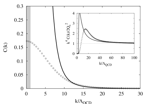
Figure 4: Value of $C(k_{\perp})$ as a function of $k_{\perp}/\Lambda_{{}_{QCD}}$ for $Q_{s}/\Lambda_{{}_{QCD}}=10$. The open circles are the result of a numerical evaluation, and the solid line is the asymptotic formula given in Eq. (82). The shaded area indicates the region where $k_{\perp}\leq\Lambda_{{}_{QCD}}$. One can see on the numerical curve the onset of saturation at low values of $k_{\perp}$. In the upper right corner, we have plotted the same data for the quantity $k_{\perp}^{4}C(k_{\perp})/2Q_{s}^{2}$, which allows for an easier reading for large values of $k_{\perp}$.

References

- [1] A.H. Mueller, Lectures given at the International Summer School on Particle Production Spanning MeV and TeV Energies (Nijmegen 99), Nijmegen, Netherlands, Aug 8-20 1999, hep-ph/9911289 .
- [2] L. McLerran, Lectures given at the 40’th Schladming Winter School: Dense Matter, March 3-10 2001, hep-ph/0104285 .
- [3] L.V. Gribov, E.M. Levin, M.G. Ryskin, Phys. Rept. 100, 1 (1983).
- [4] A.H. Mueller, J-W. Qiu, Nucl. Phys. B 268, 427 (1986).
- [5] L.L. Frankfurt, M.I. Strikman, Phys. Rept. 160, 235 (1988).
- [6] L.N. Lipatov, Sov. J. Nucl. Phys. 23, 338 (1976).
- [7] E.A. Kuraev, L.N. Lipatov, V.S. Fadin, Sov. Phys. JETP 45, 199 (1977).
- [8] I. Balitsky, L.N. Lipatov, Sov. J. Nucl. Phys. 28, 822 (1978).
- [9] J. Jalilian-Marian, A. Kovner, L. McLerran, H. Weigert, Phys. Rev. D 55, 5414 (1997).
- [10] Yu.V. Kovchegov, A.H. Mueller, Nucl. Phys. B 529, 451 (1998).
- [11] L. McLerran, R. Venugopalan, Phys. Rev. D 49, 2233 (1994).
- [12] L. McLerran, R. Venugopalan, Phys. Rev. D 49, 3352 (1994).
- [13] L. McLerran, R. Venugopalan, Phys. Rev. D 50, 2225 (1994).
- [14] Yu.V. Kovchegov, L. McLerran, Phys. Rev. D 60, 054025 (1999).
- [15] J. Jalilian-Marian, A. Kovner, A. Leonidov, H. Weigert, Nucl. Phys. B 504, 415 (1997).
- [16] J. Jalilian-Marian, A. Kovner, A. Leonidov, H. Weigert, Phys. Rev. D 59, 014014 (1999).
- [17] J. Jalilian-Marian, A. Kovner, H. Weigert, Phys. Rev. D 59, 014015 (1999).
- [18] J. Jalilian-Marian, A. Kovner, A. Leonidov, H. Weigert, Phys. Rev. D 59, 034007 (1999).
- [19] J. Jalilian-Marian, A. Kovner, A. Leonidov, H. Weigert, Erratum. Phys. Rev. D 59, 099903 (1999).
- [20] A. Kovner, G. Milhano, Phys. Rev. D 61, 014012 (2000).
- [21] A. Kovner, G. Milhano, H. Weigert, Phys. Rev. D 62, 114005 (2000).
- [22] I. Balitsky, Nucl. Phys. B 463, 99 (1996).
- [23] Yu.V. Kovchegov, Phys. Rev. D 61, 074018 (2000).
- [24] E. Iancu, A. Leonidov, L. McLerran, hep-ph/0011241 .
- [25] E. Iancu, A. Leonidov, L. McLerran, Phys. Lett. B 510, 133 (2001).
- [26] E. Iancu, L. McLerran, Phys. Lett. B 510, 145 (2001).
- [27] L. McLerran, R. Venugopalan, Phys. Rev. D 59, 094002 (1999).
- [28] A. Kovner, L. McLerran, H. Weigert, Phys. Rev. D 52, 3809 (1995).
- [29] A. Kovner, L. McLerran, H. Weigert, Phys. Rev. D 52, 6231 (1995).
- [30] A. Krasnitz, R. Venugopalan, Phys. Rev. Lett. 84, 4309 (2000).
- [31] A. Krasnitz, R. Venugopalan, Phys. Rev. Lett. 86, 1717 (2001).
- [32] A. Dumitru, L. McLerran, hep-ph/0105268.
- [33] N. Baron, G. Baur, Phys. Rev. C 48, 1999 (1993).
- [34] M. Greiner, M. Vidovic, C. Hofmann, A. Schafer, Phys. Rev. C 51, 911 (1995).
- [35] A.J. Baltz, F. Gelis, L. McLerran, A. Peshier, nucl-th/0101024, to appear in Nucl. Phys. A .
- [36] A. Kovner, U. Wiedeman, hep-ph/0106240.
- [37] D.Yu. Ivanov, A. Schiller, V.G. Serbo, Phys. Lett. B 454, 155 (1999).
- [38] R.N. Lee, A.I. Milstein, Phys. Rev. A 61, 032103 (2000).
- [39] R.N. Lee, A.I. Milstein, hep-ph/0103212 .
- [40] S.R. Klein, J. Nystrand, R. Vogt, hep-ph/0005157 .
- [41] C.S. Lam, G. Mahlon, Phys. Rev. D 62, 114023 (2000).