BARI-TH/01-418

July 2001

$D_{s}$ decays to $\eta$ and $\eta^{\prime}$ final states:
a phenomenological analysis

P. Colangelo and F. De Fazio

Istituto Nazionale di Fisica Nucleare, Sezione di Bari, Italy

Abstract

We consider the semileptonic and nonleptonic $D_{s}$ decay modes to final states with $\eta$ and $\eta^{\prime}$. We use QCD sum rules to determine the $D_{s}\to\eta$ form factor $f_{+}^{\eta}$, and a generalized factorization ansatz to compute nonleptonic decays. We propose a parameterization of possible OZI suppressed contributions producing the $\eta^{\prime}$ in the final state, compatible with current data; such a scheme can be further constrained improving the precision of the measurement of the $D_{s}$ decay rates, as expected by the ongoing experiments.

1 Introduction

The exclusive $D_{s}$ decays to final states containing $\eta$ and $\eta^{\prime}$ represent nearly $30\%$ of the total decay rate of the $D_{s}$ meson. Therefore, $D_{s}$ could be a suitable system where to gather information on important aspects of the $\eta-\eta^{\prime}$ phenomenology, namely the long-standing issue of the $\eta-\eta^{\prime}$ mixing. Moreover, $D_{s}$ can be used to further investigate some unsettled aspects of nonleptonic heavy meson decays, such as the anomalously large $\eta^{\prime}$ production observed in several heavy meson decay channels. Examples are $B^{-}\to K^{-}\eta^{\prime}$ and $D^{0}\to\overline{K}^{0}\eta^{\prime}$, the measured decay rates of which are substantially larger than what can be expected by naive theoretical calculations.

The current experimental situation concerning the $D_{s}$ transitions to $\eta$ and $\eta^{\prime}$ is summarized in Table 1 [1], mainly using the results obtained by the CLEO Collaboration in the past few years [2].

Table 1: Experimental rates and branching fractions of semileptonic and nonleptonic $D_{s}$ decays to final states containing $\eta$ and $\eta^{\prime}$.

Decay mode	$\Gamma$ $\,(10^{-15}\,GeV)$	${\cal B}(10^{-2})$
$D_{s}^{+}\to\eta\ell^{+}\nu$	$34.5\pm 9.3$	$2.6\pm 0.7$
$D_{s}^{+}\to\eta^{\prime}\ell^{+}\nu$	$11.8\pm 4.5$	$0.89\pm 0.34$
$D_{s}^{+}\to\eta\pi^{+}$	$22.6\pm 6.7$	$1.7\pm 0.5$
$D_{s}^{+}\to\eta\rho^{+}$	$143.3\pm 41.2$	$10.8\pm 3.1$
$D_{s}^{+}\to\eta^{\prime}\pi^{+}$	$51.8\pm 13.3$	$3.9\pm 1.0$
$D_{s}^{+}\to\eta^{\prime}\rho^{+}$	$134.0\pm 37.3$	$10.1\pm 2.8$

The experimental results are expected to be improved in the near future, since the analysis of the $D_{s}$ system is an important item of the experimental program of the current hadron facilities, as well as of the $e^{+}e^{-}$ machines running at the $\Upsilon(4S)$ peak.

The results in Table 1 have inspired several considerations. First, it has been proposed that information on the $\eta-\eta^{\prime}$ mixing could be obtained just considering the semileptonic decay modes. As a matter of fact, writing the hadronic matrix element governing the transition $D_{s}^{+}\to\eta\ell^{+}\nu$ in terms of form factors:

$$<\eta(p^{\prime})|{\bar{s}}\gamma_{\mu}c|D_{s}(p)>=f_{+}^{\eta}(q^{2})(p+p^{\prime})_{\mu}+f_{-}^{\eta}(q^{2})q_{\mu}$$ (1)

($q=p-p^{\prime}$) and a similar expression for $D_{s}^{+}\to\eta^{\prime}\ell^{+}\nu$, the ratio $\displaystyle{{\cal B}(D_{s}^{+}\to\eta^{\prime}\ell^{+}\nu)\over{\cal B}(D_{s}^{+}\to\eta\ell^{+}\nu)}$ could be used to access the $\eta-\eta^{\prime}$ mixing angle through the ratios of the form factors $\displaystyle{f_{\pm}^{\eta^{\prime}}(q^{2})/f_{\pm}^{\eta}(q^{2})}$ which are related to the $\eta-\eta^{\prime}$ mixing scheme [3, 4]. In particular, information could be gathered on the mixing scheme in the flavour basis [5, 6], which consists in writing the $\eta$ and $\eta^{\prime}$ states as combinations of $|\eta_{q}>=\displaystyle{1\over\sqrt{2}}|{\overline{u}}u+{\overline{d}}d>$ and $|\eta_{s}>=|{\overline{s}}s>$:

$$|\eta> = \cos\phi_{q}~{}|\eta_{q}>-\sin\phi_{s}~{}|\eta_{s}>$$

$$|\eta^{\prime}> = \sin\phi_{q}~{}|\eta_{q}>+\cos\phi_{s}~{}|\eta_{s}>\;\;\;.$$ (2)

It has been shown [5] that in this scheme a single angle is essentially required, since $|\phi_{s}-\phi_{q}|/(\phi_{s}+\phi_{q})\ll 1$, a result confirmed by a QCD sum rule calculation [7]. Therefore, one can safely assume $\phi_{s}\simeq\phi_{q}\simeq\phi$; the most recent estimates of $\phi$ give values close to $40^{0}$ [6, 8]. In the flavour scheme, the semileptonic form factors relative to $D_{s}^{+}\to\eta\ell^{+}\nu$ and $D_{s}^{+}\to\eta^{\prime}\ell^{+}\nu$ satisfy the relation

$${|f_{\pm}^{\eta^{\prime}}(q^{2})|\over|f_{\pm}^{\eta}(q^{2})|}=\cot\phi\;\;\;,$$ (3)

so that the possibility of a direct comparison with the results for $\phi$ obtained from the analyses of other channels involving $\eta-\eta^{\prime}$ particles could be envisaged. The situation is particularly simple in the case of semileptonic $D_{s}^{+}$ decays to positrons or antimuons, where essentially only the form factors $f_{+}^{\eta(\eta^{\prime})}(q^{2})$ are involved. However, in order to pursue this program, one has to neglect possible contributions to the semileptonic decay amplitude from diagrams where $\eta$ and $\eta^{\prime}$ are produced through gluon emission; we shall consider this problem below.

As for nonleptonic decays, naive factorization, using the semileptonic $D_{s}\to\eta$ and $D_{s}\to\eta^{\prime}$ form factors and the Wilson coefficients relevant for the transitions in Table 1, does not allow to predict all the branching fractions of $D_{s}^{+}\to\eta^{(\prime)}\pi^{+}$ and $D_{s}^{+}\to\eta^{(\prime)}\rho^{+}$ [9]. The same conclusion is obtained by analyzing the various decay channels in terms of transition amplitudes related by $SU(3)_{F}$ symmetry to analogous amplitudes for $D$ decays [10], or accounting for some effects of the inelastic final state rescattering [11]. In particular, the prediction for the rate of the decay mode $D_{s}^{+}\to\eta^{\prime}\rho^{+}$ is lower than the experimental measurement by more than a factor of two. This is disappointing: in Cabibbo favoured hadronic $D_{s}$ decays the final state contains a single isospin mode, thus ruling out possible interference effects due to the elastic final state interactions; moreover, the conservation of G-parity does not allow to include inelastic effects of intermediate states consisting of ordinary mesons in the $D_{s}^{+}\to\eta^{\prime}\rho^{+}$ mode [12]. Therefore, a different mechanism must be invoked to explain the enhanced $\eta^{\prime}$ production. It has been suggested that the enhancement could be due to OZI suppressed diagrams with the $\eta^{\prime}$ produced by gluons and the $c\bar{s}$ pair annihilating to a charged $W$ [3]. This mechanism would not affect substantially the $\eta$ production, since the coupling of the gluons to $\eta$ is estimated to be smaller than the coupling to $\eta^{\prime}$ [13]. However, a mechanism of this type, violating the OZI rule, could also affect the semileptonic $D_{s}^{+}\to\eta^{\prime}\ell^{+}\nu$ transition, spoiling the possibility of using the relation (3) to gather information on the angle $\phi$ from the semileptonic decay rates. Moreover, these effects could be also present in other systems, namely in $D$ decays, although in such cases the annihilation amplitudes are Cabibbo suppressed.

The effects of the gluon production of the $\eta$ and $\eta^{\prime}$, although plausible, are not included in ordinary analyses since they are difficult to take into account in a quantitative way. Nevertheless, their investigation is of particular relevance, and we shall try to perform it in a phenomenological way.

In this paper, we compute the form factor $f_{+}^{\eta}(q^{2})$ relative to $D_{s}^{+}\to\eta\ell^{+}\nu$, showing that the result is in agreement with the experimental measurement in Table 1. On the other hand, assuming the standard value of the $\eta-\eta^{\prime}$ mixing angle together with the naive factorization, other results in Table 1 are not reproduced. Therefore, we adopt a generalized factorization ansatz, fitting the relevant parameters from the experiment; moreover, we assume that the effect of the process producing the $\eta^{\prime}$ through the annihilation of the $c\bar{s}$ pair numerically modifies the $D_{s}\to\eta^{\prime}$ form factors. This enables us to investigate whether the experimental results can be reproduced by this assumption and how the reduction of the experimental uncertainty can be used to test various consequences of our ansatz.

2 QCD sum rule calculation of $f_{+}^{\eta}(q^{2})$

Let us first compute the form factor $f_{+}^{\eta}(q^{2})$ using a nonperturbative method, such as the QCD sum rule technique [14]. We adopt the usual strategy of considering a three-point function:

$$\Pi_{\mu\nu}(p^{2},p^{\prime 2},q^{2}) = i^{2}\int d^{4}x~{}d^{4}y~{}e^{-ip\cdot y}\,e^{ip^{\prime}\cdot x}\left\langle 0\right|T[J^{\eta}_{5}(x)J_{\mu}(0)J_{5}^{D_{s}}(y)]\left|0\right\rangle$$ (4)

$$= \Pi_{+}P_{\mu}+\Pi_{-}q_{\mu}\;\;\;,$$

with $J^{\eta}_{5}={\bar{s}}i\gamma_{5}s$ the pseudoscalar quark density probing the strangeness content of the $\eta$, $J_{\mu}={\bar{s}}\gamma_{\mu}c$ the weak current inducing the $c\to s$ transition, and $J_{5}^{D_{s}}={\bar{c}}i\gamma_{5}s$ a quark current having the $D_{s}$ quantum numbers. The momenta $P$ and $q$ are defined as $P=p+p^{\prime}$ and $q=p-p^{\prime}$, respectively. For the invariant function $\Pi_{+}(p^{2},p^{\prime 2},q^{2})$ a double dispersion relation in the variables $p^{2}$, $p^{\prime 2}$ can be written down:

$$\Pi_{+}(p^{2},p^{\prime 2},q^{2})={1\over\pi^{2}}\int ds_{1}\int ds_{2}\,{\rho(s_{1},s_{2},q^{2})\over(s_{1}-p^{2})(s_{2}-p^{\prime 2})}$$ (5)

where possible subtraction terms have been omitted. The spectral function $\rho(s_{1},s_{2},q^{2})$ contains, for low values of $s_{1}$ and $s_{2}$, a double $\delta-$function corresponding to the transition $D_{s}\to\eta$. Isolating such a contribution, and neglecting possible subtraction terms which we discuss later on, we can write:

$$\Pi_{+}(p^{2},p^{\prime 2},q^{2})={{\cal A}f_{+}^{\eta}(q^{2})\over(M_{D_{s}}^{2}-p^{2})(M_{\eta}^{2}-p^{\prime 2})}{f_{D_{s}}M_{D_{s}}^{2}\over m_{s}+m_{c}}+{1\over\pi^{2}}\int_{s_{1}^{0}}^{\infty}ds_{1}\int_{s_{2}^{0}}^{\infty}ds_{2}\,{\rho^{had}(s_{1},s_{2},q^{2})\over(s_{1}-p^{2})(s_{2}-p^{\prime 2})}\;.$$ (6)

In (6) we have assumed that the contribution of higher resonances and continuum of states starts from the effective thresholds $s_{1}^{0}$ and $s_{2}^{0}$. The hadronic parameter $\cal A$ represents the matrix element:

$$<0|J_{5}^{\eta}|\eta(p^{\prime})>={\cal A}$$ (7)

while the projection of the $J^{D_{s}}_{5}$ current on the $D_{s}$ state is given by the matrix element

$$<0|J_{5}^{D_{s}}|D_{s}(p)>={f_{D_{s}}M_{D_{s}}^{2}\over m_{s}+m_{c}}\;\;\;.$$ (8)

The correlator (4) can be computed in QCD for large Euclidean values of $p^{2}$ and $p^{\prime 2}$ by an Operator Product Expansion, expanding the T-product in (4) as a sum of a perturbative contribution and non perturbative terms, proportional to vacuum expectation values of quark and gluon gauge invariant operators of increasing dimension, the vacuum condensates. In practice, only the first few condensates numerically contribute, the most important ones being the dimension 3 $<{\bar{s}}s>$ and dimension 5 $<{\bar{s}}g\sigma Gs>$ condensates. The QCD expression for $\Pi_{+}$ reads:

$$\Pi_{+}(p^{2},p^{\prime 2},q^{2}) = {1\over\pi^{2}}\int_{(m_{c}+m_{s})^{2}}^{\infty}ds_{1}\int_{4m_{s}^{2}}^{\infty}ds_{2}{\rho^{pert}(s_{1},s_{2},q^{2})\over(s_{1}-p^{2})(s_{2}-p^{\prime 2})}$$ (9)

$$+ \Pi_{+}^{(D=3)}<{\overline{s}}s>+\Pi_{+}^{(D=5)}<{\overline{s}}g\sigma Gs>+...\;\;.$$

Invoking quark-hadron duality, i.e. assuming that the hadronic and the perturbative QCD spectral densities give the same result when integrated above the thresholds $s_{1}^{0}$ and $s_{2}^{0}$, we get the sum rule:

$${{\cal A}f_{D_{s}}M^{2}_{D_{s}}\over m_{s}+m_{c}}{f_{+}^{\eta}(q^{2})\over(M_{\eta}^{2}-p^{\prime 2})(M_{D_{s}}^{2}-p^{2})} = {1\over 4\pi^{2}}\int_{D}ds_{1}ds_{2}{\rho_{+}^{pert}(s_{1},s_{2},q^{2})\over(s_{1}-p^{2})(s_{2}-p^{\prime 2})}$$

$$+ \Pi_{+}^{(D=3)}<{\overline{s}}s>+\Pi_{+}^{(D=5)}<{\overline{s}}g\sigma Gs>+...$$

with

$$\rho_{+}^{pert}(s_{1},s_{2},q^{2}) = {3\over 4\sqrt{(s_{1}+s_{2}-q^{2})^{2}-4s_{1}s_{2}}}\Big{[}s_{1}-m_{c}^{2}+m_{s}^{2}+s_{2}+2m_{s}(m_{c}-m_{s})$$

$$+ 2s_{2}{(s_{1}+s_{2}-q^{2})(2s_{1}-m_{c}^{2}+m_{s}^{2})\over(s_{1}+s_{2}-q^{2})^{2}-4s_{1}s_{2}}-{(s_{1}+s_{2}-q^{2})^{2}(s_{1}-m_{c}^{2}+m_{s}^{2}+s_{2})\over(s_{1}+s_{2}-q^{2})^{2}-4s_{1}s_{2}}\Big{]}$$

and

$$\Pi_{+}^{(D=3)} = -{1\over 2}\Big{\{}{m_{c}\over rr^{\prime}}$$

$$+ (m_{c}+m_{s})\Big{[}{m_{s}^{2}\over 2rr^{\prime 2}}+{m_{c}m_{s}\over r^{2}r^{\prime}}-{m_{s}^{2}(m_{c}^{2}+m_{s}^{2}-q^{2})\over 2r^{2}r^{\prime 2}}+m_{s}^{2}\Big{(}{m_{s}^{2}\over rr^{\prime 3}}+{m_{c}^{2}\over r^{3}r^{\prime}}\Big{)}\Big{]}\Big{\}}$$

$$\Pi_{+}^{(D=5)} = {1\over 24}\Big{[}{6m_{s}^{2}(m_{c}+m_{s})\over rr^{\prime 3}}+{6m_{c}^{2}(m_{c}+m_{s})\over r^{3}r^{\prime}}$$

$$+ {2(m_{c}+m_{s})(2m_{c}^{2}+2m_{s}^{2}-2q^{2}-m_{c}m_{s})\over r^{2}r^{\prime 2}}+{12m_{c}\over r^{2}r^{\prime}}+{12m_{s}\over rr^{\prime 2}}\Big{]}\,.$$

The variables $r$ and $r^{\prime}$ are defined as $r=p^{2}-m_{c}^{2}$ and $r^{\prime}=p^{\prime}-m_{s}^{2}$. The domain $D$ is bounded by the curves

$$s_{2}^{\pm} = {[2m_{s}^{2}(s_{1}+q^{2})+\Delta(m_{c}^{2}-m_{s}^{2}-q^{2})]\over 2m_{c}^{2}}$$

$$\pm {1\over 2m_{c}^{2}}\left[\left(2m_{s}^{2}(s_{1}+q^{2})+\Delta(m_{c}^{2}-m_{s}^{2}-q^{2})\right)^{2}-4m_{c}^{2}m_{s}^{2}(s_{1}-q^{2})^{2}\right]^{1/2}$$

where $\Delta=s_{1}-m_{c}^{2}+m_{s}^{2}$, and by the lines $s_{2}=s_{2}^{0}$ and $s_{1}=s_{1}^{0}$. Eq. (2) can be improved by applying to both its sides a Borel transform, defined as follows:

$${\cal B}[{\cal F}(Q^{2})]=lim_{Q^{2}\to\infty,\;n\to\infty,\;{Q^{2}\over n}=M^{2}}\;{1\over(n-1)!}(-Q^{2})^{n}\left({d\over dQ^{2}}\right)^{n}{\cal F}(Q^{2})\;,$$ (15)

where ${\cal F}$ is a generic function of $Q^{2}$. The application of such a procedure to the sum rule amounts to exploiting the relation:

$${\cal B}\left[{1\over(s+Q^{2})^{n}}\right]={\exp(-s/M^{2})\over(M^{2})^{n}\ (n-1)!}\;,$$ (16)

with $M^{2}$ a Borel parameter. The operation, applied independently to the variables $-p^{2}$ and $-p^{\prime 2}$, improves the convergence of the series in the OPE in the r.h.s. of Eq. (9) by factorials in $n$, and, for suitably chosen values of the Borel parameters, enhances the contribution of the low-lying states in the hadronic representation of the correlator $\Pi_{+}$. Moreover, since the Borel transform of a polynomial vanishes, the procedure allows to get rid of subtraction terms in the dispersion relations, which are polynomials in $p^{2}$ or $p^{\prime 2}$. Therefore, a final sum rule can be worked out, keeping only the contribution of the lowest dimensional condensates:

$${{\cal A}f_{D_{s}}M^{2}_{D_{s}}\over m_{s}+m_{c}}f_{+}^{\eta}(q^{2})e^{-{M_{D_{s}}^{2}/M_{1}^{2}}}e^{-{M_{\eta}^{2}/M_{2}^{2}}} = {1\over 4\pi^{2}}\int_{D}ds_{1}ds_{2}\rho_{+}^{pert}(s_{1},s_{2},q^{2})e^{-{s_{1}\over M_{1}^{2}}}e^{-{s_{2}\over M_{2}^{2}}}$$

$$-e^{-{m_{c}^{2}/M_{1}^{2}}}e^{-{m_{s}^{2}/M_{2}^{2}}}{<{\bar{s}}s>\over 2}\Big{\{}m_{c} + (m_{c}+m_{s})\Big{[}-{m_{s}^{2}\over 2M_{2}^{2}}-{m_{c}m_{s}\over 2M_{1}^{2}}$$

$$- {m_{s}^{2}(m_{c}^{2}+m_{s}^{2}-q^{2})\over 2M_{1}^{2}M_{2}^{2}}+{m_{s}^{2}\over 2}\Big{(}{m_{s}^{2}\over M_{2}^{4}}+{m_{c}^{2}\over M_{1}^{4}}\Big{)}\Big{]}\Big{\}}$$

$$+e^{-{m_{c}^{2}/M_{1}^{2}}}e^{-{m_{s}^{2}/M_{2}^{2}}}{<{\bar{s}}g\sigma Gs>\over 8}\Big{[} {m_{s}^{2}(m_{c}+m_{s})\over M_{2}^{4}}+{m_{c}^{2}(m_{c}+m_{s})\over M_{1}^{4}}$$ (17)

$$+ {2(m_{c}+m_{s})(2m_{c}^{2}+2m_{s}^{2}-2q^{2}-m_{c}m_{s})\over 3M_{1}^{2}M_{2}^{2}}$$

$$- {4m_{c}\over M_{1}^{2}}-{4m_{s}\over M_{2}^{2}}\Big{]}\,.$$

In the numerical analysis of (17) we used standard values of the condensates: $<{\bar{s}}s>=0.8<{\bar{q}}q>$ with $<{\bar{q}}q>=(-0.23\;GeV)^{3}$, and $<{\bar{s}}g\sigma Gs>=m_{0}^{2}<{\bar{s}}s>$ with $m_{0}^{2}=0.8\;GeV^{2}$. The charm and strange quark masses were fixed to the values $m_{c}=1.4\,GeV$ [15] and $m_{s}=140\,MeV$ [16, 15]. As for the $D_{s}$ decay constant, we used $f_{D_{s}}=225\,MeV$ [15], while for the parameter $\cal A$ we adopted the two-point QCD sum rule result ${\cal A}=0.115\,GeV^{2}$ [7]. The obtained sum rule shows stability to the variation of the Borel parameter in the region $2.5\;GeV^{2}\leq M_{1}^{2}\leq 3.5\;GeV^{2}$ and $1.6\;GeV^{2}\leq M_{2}^{2}\leq 2.4\;GeV^{2}$, with the thresholds $s_{1}^{0}$ and $s_{2}^{0}$ in the ranges $s_{1}^{0}=5.9-6.1$ $GeV^{2}$ and $s_{2}^{0}=0.9-1.1$ $GeV^{2}$, respectively. The form factor $f_{+}^{\eta}(q^{2})$, obtained in the range of momentum transfer $0\leq q^{2}\leq 0.5$ $GeV^{2}$, is depicted in Fig. 1; it can be fitted by a linear expression

$$f_{+}^{\eta}(q^{2})=A\,q^{2}+B\,,$$ (18)

with $A=0.14$ $GeV^{-2}$ and $B=0.50\pm 0.04$. This expression is consistent, in the considered range of momentum transfer, with a polar form $\displaystyle{f_{+}^{\eta}(q^{2})={f_{+}^{\eta}(0)\over 1-{q^{2}\over M_{P}^{2}}}}$, with the mass of the pole $M_{P}\simeq 1.9$ $GeV$.

In the following, we shall consider the form factor $f_{+}^{\eta}(q^{2})$ as a theoretical input in a phenomenological analysis of $D_{s}$ transitions.

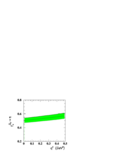
Figure 1: Form factor $f_{+}^{D_{s}\to\eta}(q^{2})$ as obtained using QCD sum rules. The shaded region represents the theoretical uncertainty related to the variation of the input parameters.

3 $D_{s}$ transitions to $\eta$ and $\eta^{\prime}$

The form factor $f_{+}^{\eta}(q^{2})$ computed above allows us to calculate the semileptonic $D_{s}^{+}\to\eta\ell^{+}\nu$ decay rate. It can also be used to analyze the nonleptonic modes $D_{s}\to\eta\pi^{+}$ and $D_{s}\to\eta\rho^{+}$ if the factorization approximation is adopted. This amounts to consider the effective Hamiltonian

$$H_{eff}={G_{F}\over\sqrt{2}}V_{cs}^{*}V_{ud}\left(C_{1}(\mu)+{C_{2}(\mu)\over N_{c}}\right)({\bar{s}}c)_{V-A}({\bar{u}}d)_{V-A}+\,h.c.\,,$$ (19)

with $({\bar{q}}_{1}q_{2})_{V-A}={\bar{q}}_{1}\gamma_{\mu}(1-\gamma_{5})q_{2}$ and $C_{1}$ and $C_{2}$ Wilson coefficients, and factorize the $V-A$ currents appearing in it. As for the modes with $\eta^{\prime}$, we further need an input on the $\eta-\eta^{\prime}$ mixing, and we choose the angle $\phi$ in the flavour basis mixing scheme, with the value $\phi=39^{0}$ coming from the measurements of $\phi\to\eta^{(\prime)}\gamma$ [17].

Table 2: Computed semileptonic and nonleptonic $D_{s}$ rates and branching fractions. Nonleptonic rates are obtained using naive factorization. The $\eta-\eta^{\prime}$ mixing is described in the flavour basis, with mixing angle $\phi=39^{0}$.

Decay mode	$\Gamma$ $\,(10^{-15}$ GeV)	${\cal B}\,(10^{-2})$
$D_{s}^{+}\to\eta\ell^{+}\nu$	$30.3\pm 4.8$	$2.3\pm 0.4$
$D_{s}^{+}\to\eta^{\prime}\ell^{+}\nu$	$12.7\pm 2.0$	$1.0\pm 0.2$
$D_{s}^{+}\to\eta\pi^{+}$	$38.5\pm 6.2$	$2.9\pm 0.5$
$D_{s}^{+}\to\eta\rho^{+}$	$74.5\pm 11.9$	$5.6\pm 0.9$
$D_{s}^{+}\to\eta^{\prime}\pi^{+}$	$33.2\pm 5.3$	$2.5\pm 0.4$
$D_{s}^{+}\to\eta^{\prime}\rho^{+}$	$30.7\pm 4.9$	$2.3\pm 0.4$

In Table 2 we collect the resulting branching fractions obtained in the factorization approximation, using $f_{\pi}=0.132$ $GeV$, $f_{\rho}=0.220$ $GeV$, $\tau_{D_{s}}=0.496\;ps$; the number of colours $N_{c}$ is fixed to $N_{c}=3$, and the values $C_{1}(m_{c})=1.263$ and $C_{2}(m_{c})=-0.513$ are chosen, corresponding to the results for the Wilson coefficients obtained at the leading order in renormalization group improved perturbation theory at $\mu=m_{c}\simeq 1.4~{}GeV$, in corrispondence to $\alpha_{s}(M_{Z})=0.118$. Using the form factor $f_{+}^{\eta}$ in (18) we obtain the branching fraction ${\cal B}(D_{s}^{+}\to\eta\ell^{+}\nu)=(2.3\pm 0.4)\times 10^{-2}$ in agreement with the experimental outcome reported in Table 1; also the result ${\cal B}(D_{s}^{+}\to\eta^{\prime}\ell^{+}\nu)=(1.0\pm 0.2)\times 10^{-2}$, obtained using Eq.(3), is within the experimental uncertainty quoted in Table 1. On the other hand, as one can infer by comparing the computed decay rates reported in Table 2 with the experimental measurements in Table 1, the calculations of the nonleptonic modes do not fit all the experimental measurements, as already anticipated by previous analyses.

In order to parameterize the deviation from the factorization approximation, as well as the possible role of the $\eta$ and $\eta^{\prime}$ gluon production, we adopt a generalized factorization ansatz, consisting in substituting the combination of the Wilson coefficients $a_{1}=C_{1}+\displaystyle{C_{2}\over N_{c}}$ with effective scale-independent parameters $a_{1}^{eff}$ in the factorized amplitudes. The coefficients $a_{1}^{eff}$ should be considered as non-universal, process-dependent parameters [18]. However, since in the decay modes $D_{s}^{+}\to\eta\pi^{+}$, $D_{s}^{+}\to\eta^{\prime}\pi^{+}$, and analogously $D_{s}^{+}\to\eta\rho^{+}$, $D_{s}^{+}\to\eta^{\prime}\rho^{+}$, the underlying process is the same, we assume only two process-dependent parameters to describe the deviation from naive factorization: $a_{1,\pi}^{eff}$ describing $D_{s}^{+}\to\eta\pi^{+}$ and $D_{s}^{+}\to\eta^{\prime}\pi^{+}$, and $a_{1,\rho}^{eff}$ describing $D_{s}^{+}\to\eta\rho^{+}$ and $D_{s}^{+}\to\eta^{\prime}\rho^{+}$.

As for the possible contribution of OZI suppressed diagrams producing $\eta$ and $\eta^{\prime}$, it is essentially related to the matrix elements $\left\langle 0\right|G{\tilde{G}}\left|\eta^{(\prime)}\right\rangle$, where $G$ is the gluon field and $\tilde{G}$ its dual. Several theoretical investigations suggest that $\left\langle 0\right|G{\tilde{G}}\left|\eta\right\rangle\ll\left\langle 0\right|G{\tilde{G}}\left|\eta^{\prime}\right\rangle$ [13, 7]; therefore, we assume that such annihilation amplitudes mainly affect the $D_{s}$ transitions to $\eta^{\prime}$. A simple parameteterizion consists in modifying the values of the parameters $A,B$ in (18), thus without affecting the shape of the form factor $f_{+}^{\eta^{\prime}}$. This seems rather reasonable, since the range of momentum transfer in $D_{s}\to\eta^{\prime}$ transitions is rather narrow ($q^{2}\simeq 0$ for $D_{s}\to\eta^{\prime}\pi$, $q^{2}=M^{2}_{\rho}$ for $D_{s}\to\eta^{\prime}\rho$ and $q^{2}<(M_{D_{s}}-M_{\eta^{\prime}})^{2}$ for $D_{s}\to\eta^{\prime}\ell\nu$), and a linear expansion is a suitable representation of the form factors. Therefore, in the case of $\eta^{\prime}$, we phenomenologically represent the $D_{s}\to\eta^{\prime}$ form factor as

$$f_{+}^{eff}(q^{2})={\bar{A}}q^{2}+{\bar{B}}\,.$$ (20)

It is now possible to use the experimental data in Table 1 to fit all the parameters we have introduced, namely $a_{1,\pi}^{eff}$, $a_{1,\rho}^{eff}$, $\bar{A}$ and $\bar{B}$. From the decays $D_{s}^{+}\to\eta\pi^{+}$ and $D_{s}^{+}\to\eta\rho^{+}$ we find that the values of $a_{1,\pi}^{eff}$ and $a_{1,\rho}^{eff}$ are bound in the ranges:

$$a_{1,\pi}^{eff}\in[0.65,1.04]\hskip 42.67912pta_{1,\rho}^{eff}\in[1.21,1.86]\,,$$ (21)

to be compared with the value of $a_{1}$ obtained from the Wilson coefficients $C_{1}$ and $C_{2}$: $\displaystyle{a_{1}(m_{c})=C_{1}(m_{c})+{C_{2}(m_{c})\over N_{c}}\simeq 1.1}$. As for the decay mode $D_{s}^{+}\to\eta^{\prime}\pi^{+}$, it involves $f_{+}^{eff}(q^{2})$; however, only the value $f_{+}^{eff}(0)={\bar{B}}$ is needed in the approximation $M_{\pi}=0$, allowing us to constrain ${\bar{B}}$ in the range

$$|{\bar{B}}|\in[0.70,1.45]\,.$$ (22)

Moreover, considering the modes $D_{s}^{+}\to\eta^{\prime}\ell^{+}\nu$ and $D_{s}^{+}\to\eta^{\prime}\rho^{+}$, we find that the relations

$$\Gamma(D_{s}^{+}\to\eta^{\prime}\rho^{+}) = X_{\rho}\left[f_{+}^{eff}(M_{\rho}^{2})\right]^{2}\left[a_{1,\rho}^{eff}\right]^{2}$$ (23)

$$\Gamma(D_{s}^{+}\to\eta^{\prime}\ell^{+}\nu) = X_{semilep}\int_{0}^{(M_{D_{s}}-M_{\eta^{\prime}})^{2}}dq^{2}\left[\lambda(M_{D_{s}}^{2},M_{\eta^{\prime}}^{2},q^{2})\right]^{3/2}\left[f_{+}^{eff}(q^{2})\right]^{2}$$ (24)

($X_{\rho}=\displaystyle{G_{F}^{2}|V_{ud}V_{cs}^{*}|^{2}f_{\rho}^{2}\over 32\pi M_{D_{s}}^{3}}\lambda(M_{D_{s}}^{2},M_{\rho}^{2},M_{\eta^{\prime}}^{2})^{3/2}$ and $X_{semilep}=\displaystyle{G_{F}^{2}V_{cs}^{2}\over 192\pi^{3}M_{D_{s}}^{3}}$) constrain the parameters ${\bar{A}}$ and ${\bar{B}}$ in selected regions of the $({\bar{B}},{\bar{A}})$ plane. These regions are delimited by two straight lines, from the datum on the nonleptonic $D_{s}^{+}\to\eta^{\prime}\rho^{+}$ decay rate, and by two ellypses corresponding to the measurement of the semileptonic $D_{s}^{+}\to\eta^{\prime}\ell^{+}\nu$ decay rate.

Considering simultaneously the constraints, all the data in Table 1 can be fitted if, in the ($\bar{B},\bar{A}$) plane, overlap regions exist among the area delimited by the ellypses from Eq.(24), the regions delimited by the straight lines from Eq.(23) and the regions between the vertical lines from Eq. (22). At the present level of accuracy of the experimental data in Table 1 such regions indeed exist. They are depicted in figure 2 and denoted as $D_{1}$, $D_{2}$, $D_{3}$ and $D_{4}$.

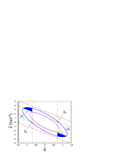
Figure 2: Bounds on the parameters $({\bar{B}},{\bar{A}})$ in (20). The ellypses represent the curves obtained from Eq. (24); the dashed lines stem from Eq. (23); the two pairs of continuous vertical lines represent the bound (22). The shaded areas and the dots indicate the regions of the parameter space satisfying all the constraints.

The regions $D_{1}$ and $D_{3}$ are defined, respectively, by the conditions:

$$-1.2\leq {\bar{B}} \leq-0.70$$ (25)

$$2.9\,[0.44-0.58{\bar{B}}]\,GeV^{-2}\leq {\bar{A}} \leq 1.38\left[-1.62{\bar{B}}+1.224\sqrt{1.57-{\bar{B}}^{2}}\right]GeV^{-2}$$

and

$$0.70\leq {\bar{B}} \leq 1.20$$ (26)

$$-1.38\left[1.62{\bar{B}}+1.224\sqrt{1.57-{\bar{B}}^{2}}\right]GeV^{-2}\leq {\bar{A}} \leq-2.9\,[0.44+0.58{\bar{B}}]\,GeV^{-2}\,.$$

On the other hand, the regions $D_{2}$ and $D_{4}$ are defined, respectively, by the conditions:

$$0.70\leq {\bar{B}} \leq 0.755$$ (27)

$$2.9\left[0.44-0.58{\bar{B}}\right]GeV^{-2}\leq {\bar{A}} \leq 1.38\,[-1.62{\bar{B}}+1.224\sqrt{1.57-\bar{B}^{2}}]\,GeV^{-2}$$

and

$$-0.755\leq {\bar{B}} \leq-0.70$$ (28)

$$-1.38\,[1.62{\bar{B}}+1.224\sqrt{1.57-\bar{B}^{2}}]\,GeV^{-2}\leq {\bar{A}} \leq-2.9\,[0.44+0.58{\bar{B}}]\,GeV^{-2}\,.$$

Although it is expected and rather plausible, the existence of such overlap regions was not guaranteed a priori; it shows that we have chosen a sensible scheme to parameterize the decays in Table 1. More important, we expect that an improvement in the accuracy of the experimental data on the $D_{s}$ decay rates would sensibly reduce the size of such overlap regions, and presumably, exclude some of them. Noticeably, already at the present level of accuracy some interesting observations can be drawn. Let us consider, for example, the parameters in the regions $D_{3}$ and $D_{2}$. In both the cases the experimental branching fraction of the semileptonic decay mode $D_{s}\to\eta^{\prime}\ell\nu$ is reproduced. However, a prime difference is that in the region $D_{3}$ the parameters $\bar{A}$ and $\bar{B}$ are opposite in sign, while in the region $D_{2}$ they have the same sign. This implies that the relation between the $D_{s}\to\eta^{\prime}$ and $D_{s}\to\eta$ form factors in (3) cannot be satisfied by the parameters in the region $D_{3}$. The same conclusion holds for the region $D_{1}$. The opposite signs between $\bar{A}$ and $\bar{B}$, as it happens in the regions $D_{1}$ and $D_{3}$, have an observable consequence in the spectrum of the semileptonic decay $D_{s}^{+}\to\eta^{\prime}\ell^{+}\nu$: in this case, a zero in the $\displaystyle{d\Gamma(D_{s}\to\eta^{\prime}\ell\nu)/dq^{2}}$ distribution should be observed, as depicted in Figure 3. On the other hand, in the case of parameters in the region $D_{2}$ (and $D_{4}$) a smooth decrease in the spectrum should be observed as in $D\to K\ell\nu$.

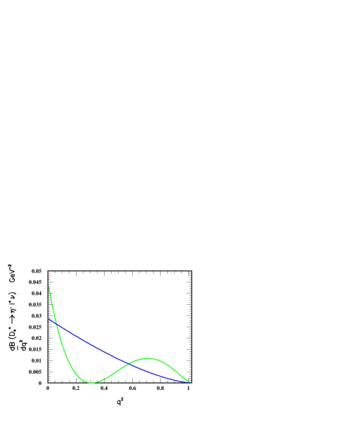
Figure 3: Semileptonic spectra of $D_{s}\to\eta^{\prime}\ell\nu$. The green curve corrisponds to the parameters $({\bar{B}},{\bar{A}})=(0.9,-2.9)\in D_{1}$, the blue one to $({\bar{B}},{\bar{A}})=(0.72,0.08)\in D_{2}$.

At the present level of accuracy of the experimental measurements, no choice can be done between the two shapes of the semileptonic distribution.

We can reasonably expect that improved data would restrict the allowed regions in the $({\bar{B}},{\bar{A}})$ plane. It could happen that they do not intersect any more, or that intersection regions could be found with restricted extension, allowing a better determination of the effective parameters introduced in our analysis. The calculation of such parameters remains a challenging task, and we do not attempt it in the present paper. However, it is worth outlining the theoretical framework in which the calculation could be carried out.

Concerning the effective coefficients $a_{1,\pi}^{eff}$ and $a_{1,\rho}^{eff}$, which take into account the deviation from the naive factorization in the corresponding decay modes, their theoretical calculation would consist in a precise determination of nonfactorizable contributions. A step in this direction has been recently performed in the case of some two-body nonleptonic B decays, where the meson picking up the B spectator quark is light, exploiting the large value of the beauty quark mass [19]. In this case, it has been observed that nonfactorizable contributions are of order $\alpha_{s}$ or $1/m_{b}$, and a QCD factorization formula has been written for the nonleptonic matrix elements in terms of meson light-cone distribution amplitudes. A possible extension of such a procedure to charm requires the development of a reliable method for computing at least the first (process dependent) $1/m_{Q}$ correction. A different approach would consist in considering the corrections to the large $N_{c}$ limit, where factorization becomes exact [20]: also in this case, however, next-to-leading $1/N_{c}$ terms are generally sizeable, and one needs their actual calculation. Therefore, it seems worth attempting to gain information on the effective coefficients from phenomenological analyses, as done, for example, in [18].

As for the OZI suppressed diagrams producing the $\eta^{\prime}$ through its coupling to the gluons, together with a weak annihilation of $D_{s}$, a perturbative calculation could be carried out in QCD, in analogy with the calculation of the $\eta^{\prime}$ production in quarkonium decays [21, 22]. The difference, in the present case, is that one has to account also for the gluon emission from a light (strange) quark, and one cannot exploit the fact that all the quarks involved are heavy, which justifies the application of perturbative QCD methods. The calculation, for small values of $q^{2}$, produces an amplitude for $D_{s}\to\eta^{\prime}\ell\nu$ of the same form as provided by a linear $q^{2}$ representation of the $D_{s}-\eta^{\prime}$ form factor. An important ingredient in this perturbative calculation is the actual value of the two-gluon-$\eta^{\prime}$ matrix element $<g(k_{1})g(k_{2})|\eta^{\prime}(p)>$ describing the vertex $\eta^{\prime}gg$ for off-shell gluons. Such a matrix element is parameterized by a form factor $F(k^{2}_{1},k^{2}_{2})$ whose value at $k^{2}_{1}=k^{2}_{2}=0$ is fixed by the QCD anomaly; as for the momentum dependence, various parameterizations have been proposed in the literature, thus providing different values for the effective parameters $\bar{A}$ and $\bar{B}$ introduced in our analysis, which in turn could correspond to various solutions for the spectrum shown in fig.3. One might notice some analogies with the analyses which explain the observed enhancement of the $\eta^{\prime}$ production in $B$ decays through the mechanism of gluon fusion [23].

All such considerations taken into account, we believe that our proposed scheme, where additional contributions are reabsorbed in the parametrization of the $D_{s}\to\eta^{\prime}$ form factor and in $a_{1,\pi}^{eff}$, $a_{1,\rho}^{eff}$ is useful from the phenomenological point of view, as a starting point for the investigation of the underlying dynamics, and could be extended to other cases.

Before concluding, we want to mention a check of consistency. If we consider the decay mode $D_{s}^{+}\to{\bar{K}}^{0}K^{+}$, which can be related to $D_{s}^{+}\to\eta\pi^{+}$ through $SU(3)_{F}$ symmetry, and describe the $D_{s}\to{\bar{K}}^{0}$ form factor by $f_{+}^{\eta}(q^{2})$, together with $f_{K}=0.160\,GeV$, we can estimate the effective parameter $a_{1,K}^{eff}$. The experimental measurement ${\cal B}(D_{s}^{+}\to{\bar{K}}^{0}K^{+})=(3.6\pm 1.1)\times 10^{-2}$ produces $a_{1,K}^{eff}\in[0.72,1.14]$, i.e. the effective parameter $a_{1,K}^{eff}$ displays a significant overlap with the range determined for $a_{1,\pi}^{eff}$. In different words, from our analysis and assuming $SU(3)_{F}$, we would be able to predict rather accurately the experimental datum for ${\cal B}(D_{s}\to{\bar{K}}^{0}K^{+})$.

4 Conclusions

We have presented a phenomenological analysis of the $D_{s}$ decays to final states containing $\eta$ and $\eta^{\prime}$. Since the theoretical investigations based on $SU(3)_{F}$ symmetry, FSI effects and standard $\eta-\eta^{\prime}$ mixing failed in simultaneously reproducing the observed branching ratios for all these decays, we have considered a possible role of annihilation diagrams, in which the $\eta^{\prime}$ is produced through its coupling to gluons. We have proposed a parametrization of those effects in the $D_{s}\to\eta^{\prime}$ form factor. As for $D_{s}\to\eta$, we used a theoretical calculation of the form factor $f_{+}^{\eta}(q^{2})$ which corresponds to a branching fraction for the decay $D_{s}\to\eta\ell\nu$ in agreement with data. A fit to all the available experimental results, adopting a generalized factorization scheme for nonleptonic decays, is possible; it constrains the parameters in restricted regions that can be discriminated by making dedicated observations, for example looking at the semileptonic spectrum of the $D_{s}\to\eta^{\prime}$ transitions. An improvement in the precision of the experimental data on $D_{s}$ decays could support this scheme and be helpful in understanding the dynamics of the $\eta$ and $\eta^{\prime}$ production in heavy meson decays.

References

[1]
D.E. Groom et al, Review of Particle Physics, Eur. Phys. J C 15
(2000) 1.
[2]
G. Brandenburg et al., CLEO Collab., Phys. Rev. Lett. 75 (1995)
3804;
C.P. Jessop et al., CLEO Collab., Phys. Rev. D 58 (1998) 052002.
[3]
R.C. Verma, A.N. Kamal and M.P. Khanna, Z. Phys. C 65 (1995) 255;
P. Ball. J.M. Frere and M. Tygat, Phys. Lett. B 365 (1996) 367.
[4]
V.V. Anisovich, D.V. Bugg, D.I. Melikhov and V.A. Novikov,
Phys. Lett. B 404 (1997) 166.
[5]
T. Feldmann, P. Kroll and B. Stech, Phys. Rev. D 58 (1998) 114006;
Phys. Lett. B 449 (1999) 339.
[6]
For a review see: T. Feldmann, Int. J. Mod. Phys.
A 15 (2000) 159.
[7]
F. De Fazio and M.R. Pennington, JHEP 0007 (2000) 051.
[8]
A. Bramon et al., Phys. Lett. B 403 (1997) 339; Eur. Phys. J. C
7 (1999) 271; Phys. Lett. B 503 (2001) 271.
[9]
M. Bauer and B. Stech, Phys. Lett. B 152 (1985) 380;
M. Bauer, B. Stech and M. Wirbel, Z. Phys. C 34 (1987) 103;
P .Bedaque, A. Das and V.S. Mathur, Phys. Rev. D 49 (1994) 269;
B. Bajc, S. Fajfer, R.J. Oakes and S. Prelovsek,
Phys. Rev. D 56 (1997) 7207.
[10]
J. Rosner, Phys. Rev. D 60 (1999) 114026.
[11]
T.N. Pham, Phys. Rev. D 46 (1992) 2080;
A.N. Kamal, Q.P. Xu and A. Czarnecki, Phys. Rev. D 48 (1993) 5215;
F. Buccella, M. Lusignoli and A. Pugliese, Phys. Lett. B 379 (1996) 249,
and references therein;
H.-Y. Cheng and B. Tseng, Phys. Rev. D 59 (1998) 014034.
[12]
H. Lipkin, Phys. Lett. B 494 (2000) 248.
[13]
V.A. Novikov, M. A. Shifman, A.I. Vainshtein and V.I. Zakharov,
Nucl. Phys. B 165 (1980) 55.
[14]
M.A. Shifman, A.I. Vainshtein and V.I. Zakharov,
Nucl. Phys. B 147 (1979) 385.
[15]
For an updated review of the QCD sum rule method and of the most recent
predictions see: P. Colangelo and A. Khodjamirian, in
“At the frontier of Particle Physics - Handbook of WCD”,
edited by M. A. Shifman, (World Scientific, Singapore) 2001, page 1495
(hep-ph/0010175).
[16]
P. Colangelo, F. De Fazio, G. Nardulli and N. Paver,
Phys. Lett. B 408 (1997) 340.
[17]
CMD-2 Collaboration, R.R. Akhmetshin et al., Phys. Lett. B 460
(1999) 242; Phys. Lett. B 473 (2000) 337;
KLOE Collaboration, M. Adinolfi et al., hep-ex/0006036;
KLOE Collaboration, A. Aloisio et al., hep-ex/0107022.
[18]
M. Neubert, V. Rieckert, B. Stech and Q.P. Xu, in Heavy Flavours,
edited by A.J. Buras and M. Lindner, (World Scientific, Singapore) 1992, and
references therein;
M. Neubert and B. Stech, in Heavy Flavours II, edited by A.J. Buras and M.
Lindner, (World Scientific, Singapore) 1998.
[19]
M. Beneke, G. Buchalla, M. Neubert and C.T. Sachrajda, Phys. Rev, Lett.
83 (1999) 1914; Nucl. Phys. B 591 (2000) 313; hep-ph/0104110.
[20]
A.J. Buras, J.-M. Gérard and R. Ruckl, Nucl. Phys. B 268 (1986) 16.
[21]
S. J. Brodsky, D. G. Coyne, T. A. DeGrand and R. R. Horgan,
Phys. Lett. B 73 (1978) 203.
[22]
J. G. Korner, J. H. Kuhn, M. Krammer and H. Schneider,
Nucl. Phys. B 229 (1983) 115.
[23]
D. Atwood and A. Soni, Phys. Lett. B 405 (1997) 150;
W. Hou and B. Tseng, Phys. Rev. Lett. 80 (1998) 434;
A. Ali, J. Chay, C. Greub and P. Ko, Phys. Lett. B 424 (1998) 161;
M. R. Ahmady, E. Kou and A. Sugamoto, Phys. Rev. D 58 (1998)
014015;
D. Du, C. S. Kim and Y. Yang, Phys. Lett. B 426 (1998) 133.