US-FT/7-01
June, 2001

The contribution of off-shell gluons
to the structure functions $F_{2}^{c}$ and $F_{L}^{c}$
and the unintegrated gluon distributions

A.V. Kotikov

Bogoliubov Laboratory of Theoretical Physics
Joint Institute for Nuclear Research
141980 Dubna, Russia

A.V. Lipatov

Department of Physics
M.V. Lomonosov Moscow State University
119899 Moscow, Russia

G. Parente

Departamento de Física de Partículas
Universidade de Santiago de Compostela
15706 Santiago de Compostela, Spain

N.P. Zotov

D.V. Skobeltsyn Institute of Nuclear Physics
M.V. Lomonosov Moscow State University
119899 Moscow, Russia

Abstract

We calculate the perturbative parts of the structure functions $F_{2}^{c}$ and $F_{L}^{c}$ for a gluon target having nonzero transverse momentum squared at order $\alpha_{s}$. The results of the double convolution (with respect to the Bjorken variable $x_{B}$ and the transverse momentum ) of the perturbative part and the unintegrated gluon densities are compared with HERA experimental data for $F_{2}^{c}$. The contribution from $F_{L}^{c}$ structure function ranges $10\div 30\%$ of that of $F_{2}^{c}$ at the kinematical range of HERA experiments.

PACS number(s): 13.60.Hb, 12.38.Bx, 13.15.Dk

1 Introduction

Recently there have been important new data on the charm structure function (SF) $F_{2}^{c}$, of the proton from the H1 [2, 5] and ZEUS [3, 4] Collaborations at HERA, which have probed the small-$x_{B}$ region down to $x_{B}=8\times 10^{-4}$ and $x_{B}=2\times 10^{-4}$, respectively. At these values of $x_{B}$, the charm contribution to the total proton SF, $F_{2}^{p}$, is found to be around $25\%$, which is a considerably larger fraction than that found by the European Muon Collaboration at CERN [6] at larger $x_{B}$, where it was only $\sim 1\%$ of $F_{2}^{p}$. Extensive theoretical analyses in recent years have generally served to confirm that the $F_{2}^{c}$ data can be described through perturbative generation of charm within QCD (see, for example, the review in Ref. [7] and references therein).

In the framework of DGLAP dynamics [8, 9] there are two basic methods to study heavy flavour physics. One of them [10] is based on the massless evolution of parton distributions and the other [11] on the boson-gluon fusion process. There are also interpolating schemes (see Ref. [12] and references therein). The present HERA data [2, 3, 4, 5] for the charm SF $F_{2}^{c}$ are in good agreement with the predictions from Ref. [11].

We note, however, that perhaps more relevant analyses of the HERA data, where the $x_{B}$ values are quite small, are those based on BFKL dynamics [13] (see discussions in the review of Ref. [14] and references therein), because the leading $ln(1/x_{B})$ contributions are summed. The basic dynamical quantity in BFKL approach is the unintegrated gluon distribution $\varphi_{g}(x,k^{2}_{\bot})$ ($f_{g}$ is the (integrated) gluon distribution multiplied by $x_{B}$ and $k_{\bot}$ is the transverse momentum)

$$f_{g}(x_{B},Q^{2})~{}=~{}\int^{Q^{2}}\frac{dk^{2}_{\bot}}{k^{2}_{\bot}}\;\varphi_{g}(x_{B},k^{2}_{\bot})~{}~{}~{}~{}~{}\mbox{(hereafter}~{}q^{2}=-Q^{2},~{}k^{2}=-k^{2}_{\bot}~{}~{}\mbox{)},$$ (1)

which satisfies the BFKL equation.

We define the Bjorken variables

$$x_{B}=Q^{2}/(2pq)~{}~{}~{}\mbox{ and }~{}~{}~{}x=Q^{2}/(2kq),$$ (2)

for lepton-hadron and lepton-parton scattering, respectively, where $p^{\mu}$ and $k^{\mu}$ are the hadron and the gluon 4-momentums, respectively, and $q^{\mu}$ is the photon 4-momentum.

Notice that the integral is divergent at the lower limit and so it leads to the necessity to consider the difference $f_{g}(x_{B},Q^{2})-f_{g}(x_{B},Q^{2}_{0})$ with some nonzero $Q^{2}_{0}$ (see discussions in Sect. 3), i.e.

$$f_{g}(x_{B},Q^{2})~{}=~{}f_{g}(x_{B},Q^{2}_{0})+\int^{Q^{2}}_{Q^{2}_{0}}\frac{dk^{2}_{\bot}}{k^{2}_{\bot}}\;\varphi_{g}(x_{B},k^{2}_{\bot})$$ (3)

In our analysis below we will not use the Sudakov decomposition, which is sometimes quite convenient in high-energy calculations. However, it is useful to have relations between our calculations and the results, where the Sudakov decomposition has been used. The corresponding analysis will be done in the next Section. Here we only note that the property $k^{2}=-k^{2}_{\bot}$ (see Eq. (1)) comes from the fact that the Bjorken parton variable $x$ in the standard and in the Sudakov approaches coincide.

Then, in the BFKL approach the SFs $F^{c}_{2,L}(x_{B},Q^{2})$ are driven at small $x_{B}$ by gluons and are related in the following way to the unintegrated distribution $\varphi_{g}(x,k^{2}_{\bot})$:

$$F^{c}_{2,L}(x_{B},Q^{2})~{}=~{}\int^{1}_{x_{B}}\frac{dx}{x}\int\frac{dk^{2}_{\bot}}{k^{2}_{\bot}}\;C^{g}_{2,L}(x,Q^{2},m_{c}^{2},k^{2}_{\bot})~{}\varphi_{g}(x_{B}/x,k^{2}_{\bot}),$$ (4)

The functions $C^{g}_{2,L}(x,Q^{2},m_{c}^{2},k^{2}_{\bot})$ may be regarded as the structure functions of the off-shell gluons with virtuality $k^{2}_{\bot}$ (hereafter we call them as coefficient functions). They are described by the quark box (and crossed box) diagram contribution to the photon-gluon interaction (see Fig. 1).

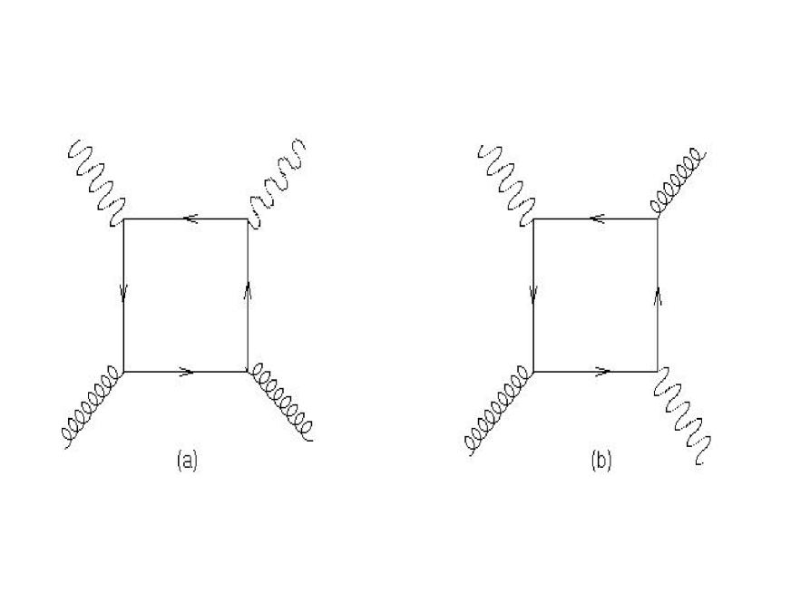
Figure 1: The diagrams contributing to $T_{\mu\nu}$ for a gluon target. They should be multiplied by a factor of 2 because of the opposite direction of the fermion loop. The diagram (a) should be also doubled because of crossing symmetry.

The purpose of the article is to calculate these coefficient functions $C^{g}_{2,L}(x,Q^{2},m_{c}^{2},k^{2}_{\bot})$ and to analyze experimental data for $F^{c}_{2}(x_{B},Q^{2})$ by applying Eq. (4) with different sets of unintegrated gluon densities (see Ref. [15]) and to give predictions for the longitudinal SF $F^{c}_{L}(x_{B},Q^{2})$.

It is instructive to note that the diagrams shown in Fig. 1. are similar to those of the photon-photon scattering process. The corresponding QED contributions have been calculated many years ago in Ref. [16] (see also the beautiful review in Ref. [17]). Our results have been calculated independently and they are in full agreement with Ref. [16] (see Appendix B). However, we hope that our formulas which are given in a more simple form could be useful for others.

The structure of this article is as follows: in Sect. 2 we present the basic formalism of our approach with a brief review of the calculational steps (based on Ref. [18]). The connection of our analysis with the Sudakov-like approach is also given. Later, we present the results for the two most important polarization matrices for off-shell gluons into the proton. In Sect. 3 and 4 we give the predictions for the structure functions $F_{2}^{c}$ and $F_{L}^{c}$ for two cases of unintegrated gluon distribution functions (see Ref. [15]) used, which are shortly reviewed. In Appendix A we show the basic technique for the evaluation of the required Feynman diagrams. Appendix B contains the review of QED results from Refs. [16, 17]. In Appendix C we consider the limiting cases, when the values of the quark mass or the gluon momentum are equal to zero and also when the value of the photon “mass” $Q^{2}$ goes to zero.

2 Approach

The hadron part of the deep inelastic (DIS) spin-average lepton-hadron cross section can be represented in the form :

$$F_{\mu\nu}~{}=~{}e_{\mu\nu}(q)~{}F_{L}(x_{B},Q^{2})+d_{\mu\nu}(q,p)~{}F_{2}(x_{B},Q^{2}),$$ (5)

where $q^{\mu}$ and $p^{\mu}$ are the photon and hadron momenta,

$$e_{\mu\nu}(q)=g_{\mu\nu}-\frac{q_{\mu}q_{\nu}}{q^{2}}~{}~{}\mbox{ and }~{}~{}d_{\mu\nu}(q,p)=-\Biggl{[}g_{\mu\nu}+2x_{B}\frac{(p_{\mu}q_{\nu}+p_{\nu}q_{\mu})}{q^{2}}+p_{\mu}p_{\nu}\frac{4x_{B}^{2}}{q^{2}}\Biggr{]}$$

and $F_{k}(x_{B},Q^{2})~{}~{}($hereafter $k=2,L)$ are structure functions.

The tensor $F_{\mu\nu}$ is connected via the optical theorem with the amplitude of elastic forward scattering of a photon on a hadron $T_{\mu\nu}(q,p)$, which may be decomposed in invariant amplitudes $T_{k}(x_{B},Q^{2})$ by analogy with Eq. (5).

Let us expand the invariant amplitudes in inverse powers of $x_{B}$:

$$T_{k}~{}=~{}\sum_{n=0}^{\infty}{\biggl{(}\frac{1}{x_{B}}\biggr{)}}^{n}\;T_{k,n}$$ (6)

The coefficients $T_{k,n}$ coincide (for even $n$) with the moments $M_{k,n}$ of the SF $F_{k}$:

$$T_{k,n}~{}=~{}M_{k,n}\equiv\int_{0}^{1}dz~{}z^{n-2}F_{k}(z,Q^{2})~{}~{}~{}$$ (7)

2.1 Evaluation of coefficient functions

We would like to note that the previous formalism can be replicated at parton level by replacing the hadron momentum $p^{\mu}$ by the gluon one $k^{\mu}$ and the Bjorken variable $x_{B}$ by the corresponding $x$. Then, the hadron part of the deep inelastic spin-average lepton-parton cross section can be represented in the form

$$F^{p}_{\mu\nu}~{}=~{}e_{\mu\nu}(q)~{}F^{p}_{L}(x,Q^{2})+d_{\mu\nu}(q,k)~{}F^{p}_{2}(x,Q^{2}),$$ (8)

where $F^{p}_{k}(x,Q^{2})$ are the structure functions of lepton-parton DIS.

As in our analysis we only consider gluons, the unintegrated gluon distribution into the parton (i.e. into the gluon) $\varphi^{p}_{g}(x,k^{2}_{\bot})$ should have the form

$$\varphi^{g}_{g}(x,k^{2}_{\bot})~{}=~{}\delta(1-x)\hat{\varphi}(k^{2}_{\bot}),$$

where $\hat{\varphi}(k^{2}_{\bot})$ is a function of $k^{2}_{\bot}$.

The parton SF $F^{p}_{k}(x,Q^{2})$ and the amplitudes $T_{k}^{p}(x,Q^{2})$ at the parton level obey equations similar to Eq. (6) and Eq. (7) with the replacement $x_{B}\to x$. Then, they are connected via optical theorem:

$$T_{k}^{p}(x,Q^{2})~{}=~{}\sum_{n=0}^{\infty}{\biggl{(}\frac{1}{x}\biggr{)}}^{n}\;\int_{0}^{1}dz~{}z^{n-2}F_{k}^{p}(z,Q^{2})~{}~{}~{}~{}~{}~{}(n=2m)$$ (9)

Thus, the coefficient functions $C^{g}_{k}(x,Q^{2},k^{2})$ of the parton SF $F^{p}_{k}(x,Q^{2})$

$$F^{p}_{2,L}(x,Q^{2})~{}=~{}\int\frac{dk^{2}_{\bot}}{k^{2}_{\bot}}\;C^{g}_{2,L}(y,Q^{2},m_{c}^{2},k^{2}_{\bot})\Theta(x_{0}-x)~{}\hat{\varphi}(k^{2}_{\bot}),$$ (10)

can be obtained directly using the amplitudes $T_{k}^{p}(x,Q^{2})$ at the parton level

$$T^{p}_{2,L}(x,Q^{2})~{}=~{}\int\frac{dk^{2}_{\bot}}{k^{2}_{\bot}}\;\tilde{C}^{g}_{2,L}(y,Q^{2},m_{c}^{2},k^{2}_{\bot})~{}\hat{\varphi}(k^{2}_{\bot}),$$ (11)

in the following way:

$$\tilde{C}^{g}_{k}(x,Q^{2},k^{2})~{}=~{}\sum_{n=0}^{\infty}{\biggl{(}\frac{1}{x}\biggr{)}}^{n}\;\int_{0}^{1}dz~{}z^{n-2}C^{g}_{k}(z,Q^{2},k^{2})\Theta(z_{0}-z),$$ (12)

where we have extracted a kinematical factor $\Theta(z_{0}-z)$.

As it was already discussed we will work with gluon part alone, keeping nonzero values of quark masses and the gluon virtuality. The corresponding Feynman diagrams are displayed on Fig. 1. The coefficient functions $C^{g}_{k}(x,Q^{2},k^{2})$ do not depend on the target type. So, it can be calculated in photon-parton DIS and used later in the photon-hadron reaction (see Eq. (4)).

2.2 Connection with the Sudakov-like approach

One of the basic ingredients in the Sudakov-like approach is the introduction of an additional light-cone momentum $n^{\mu}$ with $n^{2}=0$ and $(np)=1$.

The gluon momentum $k^{\mu}$ can be represented as

$$k^{\mu}=\xi p^{\mu}+\frac{k^{2}+k^{2}_{\bot}}{2\xi}n^{\mu}+k_{T}^{\mu}$$ (13)

with the following properties

$$p^{2}=n^{2}=(pk_{T})=(nk_{T})=0,~{}~{}~{}(np)=1$$ (14)

where the four-vector $k^{\mu}_{T}$ contains only the transverse part of $k^{\mu}$, $k_{T}=(0,k_{\bot},0)$, i.e. $k_{T}^{2}=-k^{2}_{\bot}$. and $\xi=x_{B}/x$ is the fraction of the proton momentum carried by the gluon (see Eq. (4).

To study the relations between the “usual” approach used here and the Sudakov-like one, it is convenient to introduce the following parametrization for the vector $n^{\mu}$ (see Ref. [19])

$$n^{\mu}~{}=~{}\frac{2x_{B}}{Q^{2}}\left(x_{B}p^{\mu}+q^{\mu}\right)$$ (15)

It is easy to check that the properties in Eq. (14) are fulfilled.

Then, for the scalar product $(kq)$ we have in the Sudakov-like approach:

$$(kq) = \xi\;(pq)+\frac{k^{2}+k^{2}_{\bot}}{2\xi}\;(nq)$$ (16)

$$= \frac{Q^{2}}{2x}\left[1-x^{2}\frac{k^{2}+k^{2}_{\bot}}{Q^{2}}\right]$$

If $k^{2}=-k^{2}_{\bot}$, then it follows from Eq. (16)

$$x~{}=~{}\frac{Q^{2}}{2(kq)},$$

that agrees with Eq. (2). Also from Eq. (13) it follows

$$k^{\mu}=xp^{\mu}+k_{T}^{\mu},$$ (17)

where $x$ is the fraction of the proton momentum carried by the gluon.

2.3 Feynman-gauge gluon polarization

As a first approximation we consider gluons having polarization tensor (hereafter the indices $\alpha$ and $\beta$ are connected with gluons and $\mu$ and $\nu$ are connected with photons):

$$\hat{P}^{\alpha\beta}=-g^{\alpha\beta}$$ (18)

This polarization tensor corresponds to the case when gluons do not interact. In some sense the case of polarization is equal to the standard DIS suggestions about parton properties, excepting their off-shell property. The polarization in Eq. (18) gives the main contribution to the polarization tensor we are interested in (see below)

$$\hat{P}^{\alpha\beta}_{BFKL}=\frac{k_{\bot}^{\alpha}k_{\bot}^{\beta}}{k_{\bot}^{2}}=\frac{x^{2}}{-k^{2}}p^{\alpha}p^{\beta},~{}~{}~{}$$ (19)

which comes from the high energy (or $k_{T}$) factorization prescription [20, 21, 22] .

Contracting the photon projectors (connected with photon indices of diagrams in Fig.1.)

$$\hat{P}^{(1)}_{\mu\nu}=-\frac{1}{2}g_{\mu\nu}~{}~{}\mbox{ and }~{}~{}\hat{P}^{(2)}_{\mu\nu}=4x^{2}\frac{k_{\mu}k_{\nu}}{Q^{2}}$$

with the hadronic tensor $F_{\mu\nu}$, we obtain the following relations at the parton level (i.e. for off-shell gluons having momentum $k_{\mu}$)

$$\tilde{\beta}^{2}\;C^{g}_{2}(x) = {\cal K}\;\left[f^{(1)}+\frac{3}{2\tilde{\beta}^{2}}\;f^{(2)}\right]$$ (20)

$$\tilde{\beta}^{2}\;C^{g}_{L}(x) = {\cal K}\;\left[4bx^{2}f^{(1)}+\frac{(1+2bx^{2})}{\tilde{\beta}^{2}}\;f^{(2)}\right]~{}=~{}{\cal K}\;f^{(2)}+4bx^{2}\tilde{\beta}^{2}\;C^{g}_{2},$$ (21)

where the normalization factor ${\cal K}=e_{c}^{2}\;\alpha_{s}(Q^{2})/(4\pi)\;x$,

$$P^{(i)}_{\mu\nu}F_{\mu\nu}={\cal K}\;f^{(i)},\,i=1,2$$

and $\tilde{\beta}^{2}=1-4bx^{2},~{}~{}b=-k^{2}/Q^{2}\equiv k_{\bot}^{2}/Q^{2}>0,~{}~{}a=m^{2}/Q^{2}$. The kinematical factor $z_{0}$ which appear in Eq. (12) is

$$z_{0}~{}=~{}\frac{1}{1+4a+b}$$ (22)

Applying the projectors $\hat{P}^{(i)}_{\mu\nu}$ to the Feynman diagrams displayed in Fig.1, we obtain the following results for the contributions to expressions

$$f^{(1)} = -2\beta\Biggl{[}1-\biggl{(}1-2x(1+b-2a)\;[1-x(1+b+2a)]\biggr{)}\;f_{1}$$ (23)

$$+ (2a-b)(1-2a)x^{2}\;f_{2}\Biggr{]},$$

$$f^{(2)} = 8x\;\beta\Biggl{[}(1-(1+b)x)-2x\biggl{(}bx(1-(1+b)x)(1+b-2a)+a\tilde{\beta}^{2}\biggr{)}\;f_{1}$$ (24)

$$+ bx^{2}(1-(1+b)x)(2a-b)\;f_{2}\Biggr{]},$$

where

$$\beta^{2}=1-\frac{4ax}{(1-(1+b)x)}$$

and

$$f_{1}=\frac{1}{\tilde{\beta}\beta}\;ln\frac{1+\beta\tilde{\beta}}{1-\beta\tilde{\beta}},~{}~{}~{}~{}~{}f_{2}=\frac{-4}{1-\beta^{2}\tilde{\beta}^{2}}$$

The important regimes: $k^{2}=0$, $m^{2}=0$ and $Q^{2}\to 0$ are considered in Appendix C. The $Q^{2}=0$ limit is given in Sect. 2.5.

2.4 BFKL-like gluon polarization

Now we take into account the BFKL gluon polarization given in Eq. (19). As we already noted in previous subsection, in these calculations we did not use Sudakov decomposition and, hence, the hadron momentum $p^{\alpha}$ is not so convenient variable in our case. Thus, we represent the projector $\hat{P}^{\alpha\beta}_{BFKL}$ as a combination of projectors constructed by the momenta $k^{\alpha}$ and $q^{\alpha}$.

We can represent the tensor $F^{\alpha\beta}$ in the general form:

$$F^{\alpha\beta}~{}=~{}Ag^{\alpha\beta}+Bq^{\alpha}q^{\beta}+Ck^{\alpha}k^{\beta}+D\left(k^{\alpha}q^{\beta}+q^{\alpha}k^{\beta}\right),$$ (25)

where $A$, $B$, $C$ and $D$ are some scalar functions of the variables $y$, $a$ and $b$.

¿From the gauge invariance of the vector current: $k^{\alpha}F^{\alpha\beta}=k^{\beta}F^{\alpha\beta}=0$ we have the following relations

$$C\;k^{2}~{}=~{}-\left[A+D\;(kq)\right],~{}~{}~{}B\;(kq)~{}=~{}-D\;k^{2}$$ (26)

If we apply the BFKL-like projector $\hat{P}^{\alpha\beta}_{BFKL}$ and use the light-cone properties given in Eq. (14), we get the simple relation

$$\hat{P}^{\alpha\beta}_{BFKL}F^{\alpha\beta}~{}=~{}D\;(kq)$$ (27)

The standard projectors $g^{\alpha\beta}$ and $q^{\alpha}q^{\beta}$ lead to the relations

$$g^{\alpha\beta}F^{\alpha\beta} = 3A+D\frac{Q^{2}}{2x}\tilde{\beta}^{2}$$ (28)

$$q^{\alpha}q^{\beta}F^{\alpha\beta} = \frac{\tilde{\beta}^{2}}{bx^{2}}\left[3A+D\frac{Q^{2}}{2x}\tilde{\beta}^{2}\right]$$ (29)

¿From Eqs. (26), (28) and (29) we have

$$\left[\left((kq)^{2}-k^{2}q^{2}\right)g^{\alpha\beta}+3k^{2}q^{\alpha}q^{\beta}\right]F^{\alpha\beta}~{}=~{}-D\frac{Q^{8}}{4x^{4}}\tilde{\beta}^{4}$$ (30)

and the BFKL-like projector $\hat{P}^{\alpha\beta}_{BFKL}$ can be represented as

$$\hat{P}^{\alpha\beta}_{BFKL}~{}=~{}-\frac{1}{2}\frac{1}{\tilde{\beta}^{4}}\left[\tilde{\beta}^{2}g^{\alpha\beta}-12bx^{2}\frac{q^{\alpha}q^{\beta}}{Q^{2}}\right]$$ (31)

In the previous section we have already calculated the contributions to coefficient functions using the first term within the brackets in the r.h.s. of Eq. (31). Repeating the above calculations with the projector $\sim q^{\alpha}q^{\beta}$, we obtain the total contribution to the coefficient functions which can be represented as the following shift in the results given in Eqs. (20)- (24):

$$C^{g}_{2}(x)~{} \to ~{}C^{g}_{2,BFKL}(x),~{}~{}~{}C^{g}_{L}(x)~{}\to~{}C^{g}_{L,BFKL}(x);$$

$$f^{(1)}~{} \to ~{}f^{(1)}_{BFKL}=\frac{1}{\tilde{\beta}^{4}}\left[\tilde{\beta}^{2}f^{(1)}~{}-~{}3bx^{2}\tilde{f}^{(1)}\right]$$

$$f^{(2)}~{} \to ~{}f^{(2)}_{BFKL}=\frac{1}{\tilde{\beta}^{4}}\left[\tilde{\beta}^{2}f^{(2)}~{}-~{}3bx^{2}\tilde{f}^{(2)}\right],$$ (32)

where

$$\tilde{f}^{(1)} = -\beta\Biggl{[}\frac{1-x(1+b)}{x}-2\biggl{(}x(1-x(1+b))(1+b-2a)+a\tilde{\beta}^{2}\biggr{)}\;f_{1}$$ (33)

$$- x(1-x(1+b))(1-2a)\;f_{2}\Biggr{]},$$

$$\tilde{f}^{(2)} = 4\;\beta~{}(1-(1+b)x)^{2}\Biggl{[}2-(1+2bx^{2})\;f_{1}-bx^{2}\;f_{2}\Biggr{]},$$ (34)

For the important regimes when $k^{2}=0$, $m^{2}=0$ and $Q^{2}\to 0$, the analyses are given in Appendix C.

Notice that our results in Eqs. (33) and (34) should coincide with the integral representations of Refs. [20, 26] (at $Q^{2}\to 0$ there is full agreement (see following subsection) with the formulae of Refs. [20, 26] for photoproduction of heavy quarks). Our results in Eqs. (33) and (34) should also agree with those in Ref. [25] but the direct comparison is quite difficult because the authors of Ref. [25] used a different (and quite complicated) way to obtain their results and the structure of their results is quite cumbersome (see Appendix A in Ref. [25]). We have found numerical agreement in the case of $F_{2}(x_{B},Q^{2})$ (see Sect. 3 and Fig.4).

2.5 $Q^{2}=0$ limit and Catani-Ciafaloni-Hautmann approach

We introduce the new variables $\hat{s}$, $\rho$ and $\Delta$ which are useful in the limit $Q^{2}\to 0$:

$$\hat{s}=\frac{Q^{2}}{x},~{}~{}\rho=4ax\equiv\frac{4m^{2}}{\hat{s}},~{}~{}\Delta=bx\equiv\frac{-k^{2}}{Q^{2}}x=\frac{k^{2}_{\bot}}{\hat{s}}$$ (35)

and express our formulae above as functions of $\rho$ and $\Delta$ at small $x$ asymptotic (i.e. small $Q^{2}$).

When $x=0$ we have got the following relations:
for the intermediate functions

$$\tilde{\beta}^{2} = 1,~{}~{}\beta^{2}=1-\frac{\rho}{1-\Delta}\equiv\hat{\beta}^{2},~{}~{}f_{1}=\frac{1}{\hat{\beta}}ln\frac{1+\hat{\beta}}{1-\hat{\beta}}\equiv L(\hat{\beta}),~{}~{}f_{2}=\frac{4\hat{\beta}}{\rho}(1-\Delta)$$ (36)

$$f^{(1)} = 2\hat{\beta}\Biggl{[}\left(1+\rho-\frac{\rho^{2}}{2}\right)L(\hat{\beta})-(1-\rho)+\left(2+\rho-2L(\hat{\beta})\right)\Delta$$ (37)

$$+ 2\left(L(\hat{\beta})-1\right)\Delta^{2}\Biggr{]},$$

$$x\tilde{f}^{(1)} = -2\hat{\beta}\Biggl{[}2(1-\Delta)-\rho L(\hat{\beta})\Biggr{]},~{}~{}~{}f^{(2)}~{}=~{}x\tilde{f}^{(2)}~{}=~{}0,$$ (38)

and, thus, for the coefficient functions

$$C^{g}_{L}~{}=~{}0,~{}~{}~{}~{}~{}C^{g}_{2}~{}=~{}{\cal K}\;f^{(1)}_{BFKL},$$ (39)

where

$$f^{(1)}_{BFKL} = 2\hat{\beta}\Biggl{[}\left(1+\rho-\frac{\rho^{2}}{2}\right)L(\hat{\beta})-(1+\rho)+\left(8+\rho-(2+3\rho)L(\hat{\beta})\right)\Delta$$ (40)

$$+ 2\left(L(\hat{\beta})-4\right)\Delta^{2}\Biggr{]},$$

We note that the results coincide exactly with those from Catani-Ciafaloni-Hautmann work in Ref. [20, 26] (see Eq. (2.2) in Ref. [26]) in the case of photoproduction of heavy quarks. The $O(x)$ contribution in the $Q^{2}\to 0$ limit is given in Appendix C (see subsection C.3).

3 Comparison with $F_{2}^{c}$ experimental data

With the help of the results obtained in the previous Section we have analyzed HERA data for SF $F_{2}^{c}$ from ZEUS [4] and H1 [5] collaborations.

3.1 Unintegrated gluon distribution

In this paper we consider two different parametrizations for the unintegrated gluon distribution  [15]. Firstly, we use the parametrization based on the numerical solution of the BFKL evolution equation [27] (RS–parametrization). The solution has the following form [27]:

$$\Phi(x,k^{2}) {=} \frac{a_{1}}{a_{2}+a_{3}+a_{4}}\left[a_{2}+a_{3}\;\frac{Q_{0}^{2}}{k^{2}}+\left(\frac{Q_{0}^{2}}{k^{2}}\right)^{2}+\alpha\;x+\frac{\beta}{\epsilon+\ln(1/x)}\right]$$ (41)

$$C_{q}{\left[\frac{a_{5}}{a_{5}+x}\right]}^{1/2}\left[1-a_{6}x^{a_{7}}\ln{(k^{2}/a_{8})}\right](1+a_{11}x)(1-x)^{a_{9}+a_{10}\ln(k^{2}/a_{8})},$$

where

$$C_{q}=\cases{1,&$\mbox{if}\quad k^{2}<q_{0}^{2}(x)$,\cr q_{0}^{2}(x)/k^{2},&$\mbox{if}\quad k^{2}>q_{0}^{2}(x)$}$$ (42)

The parameters $(a_{1}-a_{11},\alpha,\beta$ and $\epsilon)$ were found (see Ref. [27]) by minimization of the differences between the l.h.s and the r.h.s. of the BFKL-type equation for the unintegrated gluon distribution $\Phi(x,k^{2})$ with ‘$Q_{0}^{2}=$4 GeV².

Secondly, we also use the results of a BFKL-like parametrization of the unintegrated gluon distribution $\Phi(x,k_{\bot}^{2},\mu^{2})$, according to the prescription given in Ref. [28]. The proposed method lies upon a straightforward perturbative solution of the BFKL equation where the collinear gluon density $x\,G(x,\mu^{2})$ from the standard GRV set [29] is used as the boundary condition in the integral form of Eq. (1). Technically, the unintegrated gluon density is calculated as a convolution of the collinear gluon density $G(x,\mu^{2})$ with universal weight factors [28]:

$$\Phi(x,k_{\bot}^{2},\mu^{2})=\int_{x}^{1}{\cal G}(\eta,k_{\bot}^{2},\mu^{2})\,\frac{x}{\eta}\,G(\frac{x}{\eta},\mu^{2})\,d\eta,$$ (43)

where

$${\cal G}(\eta,k_{\bot}^{2},\mu^{2})=\frac{\bar{\alpha}_{s}}{\eta k_{\bot}}\,\cases{J_{0}(2\sqrt{\bar{\alpha}_{s}\ln(1/\eta)\ln(\mu^{2}/k^{2}_{\bot})}),&$\mbox{if}\quad k^{2}_{\bot}<\mu^{2}$,\cr I_{0}(2\sqrt{\bar{\alpha}_{s}\ln(1/\eta)\ln(k^{2}_{\bot}/\mu^{2})}),&$\mbox{if}\quad k^{2}_{\bot}>\mu^{2}$},$$ (44)

20xun01 where $J_{0}$ and $I_{0}$ stand for Bessel functions (of real and imaginary arguments, respectively), and $\bar{\alpha}_{s}=3{\alpha}_{s}/\pi$. The parameter $\bar{\alpha}_{s}$ is connected with the Pomeron trajectory intercept: $\Delta_{P}=\bar{\alpha}_{s}4\ln{2}$ in the LO and $\Delta_{P}=\bar{\alpha}_{s}4\ln{2}-N\bar{\alpha}_{s}^{2}$ in the NLO approximations, where $N$ is a number, $N\sim 18$ [30]-[32]. However, some resummation procedures proposed in the last years lead to positive value of $\Delta_{P}\sim 0.2-0.3$ (see Refs. [33, 34] and references therein).

Therefore, in our calculations with Eq. (43) we only used the solution of the LO BFKL equation and considered $\Delta_{P}$ as a free parameter varying it from 0.166 to 0.53. This approach was used for the description of the $p_{T}$ spectrum of $D^{*}$ meson electroproduction at HERA [35] where the value for the Pomeron intercept parameter $\Delta_{P}=0.35$ was obtained . We used this value of $\Delta_{P}$ in our present calculations with $\mu^{2}=Q_{0}^{2}=1-4$ GeV².

3.2 Numerical results

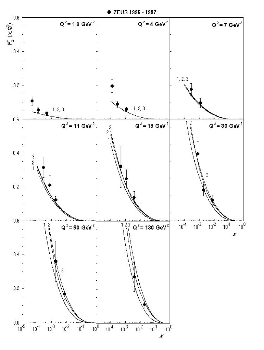
Figure 2: The structure function $F_{2}^{c}(x,Q^{2})$ as a function of $x$ for different values of $Q^{2}$ compared to ZEUS data [4]. Curves 1, 2 and 3 correspond to SF obtained in the standard parton model with the GRV  [29] gluon density at the leading order approximation and to SF obtained in the $k_{T}$ factorization approach with RS [27] and BFKL (at $Q_{0}^{2}=4$ GeV²) [28] parametrizations of unintegrated gluon distribution.

For the calculation of the SF $F_{2}^{c}$ we use Eq. (4) in the following form:

$$F_{2}^{c}(x,Q^{2}) = \int_{x(1+4a)}^{1}\frac{dy}{y}C_{2}^{g}(\frac{x}{y},Q^{2},0)\,yG(y,Q_{0}^{2})+$$ (45)

$$+ \sum_{i=1}^{2}\int_{y_{min}^{(i)}}^{y_{max}^{(i)}}\frac{dy}{y}\int_{k_{{\bot}min}^{2(i)}}^{k_{{\bot}max}^{2(i)}}dk_{\bot}^{2}\,C_{2}^{g}(\frac{x}{y},Q^{2},k_{\bot}^{2})\,\Phi(y,k_{\bot}^{2},Q_{0}^{2}).$$

Here $\Phi(y,k_{\bot}^{2},Q_{0}^{2})=\frac{1}{k_{\bot}^{2}}\varphi_{g}(y,k_{\bot}^{2},Q_{0}^{2})$ and the changes $x_{B}\to x,x\to y$ were done in comparison with Eq. (4). The coefficient function $C_{2}^{g}(x)$ is given in Eq. (20) with $f^{(1)}_{BFKL}$ and $f^{(2)}_{BFKL}$ instead of $f^{(1)}$ and $f^{(2)}$, respectively (see Eq. (32)). The functions $f^{(1)}$ and $f^{(2)}$ in Eq. (20) are given by Eqs. (23) and (24), respectively, and the functions $\tilde{f}^{(1)}$ and $\tilde{f}^{(2)}$ can be found in Eqs. (33) and (34), respectively.

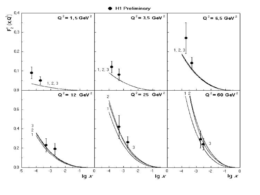
Figure 3: The structure function $F_{2}^{c}(x,Q^{2})$ as a function of $x$ for different values of $Q^{2}$ compared to H1 data [5]. Curves 1, 2 and 3 are as in Fig. 2.

The integration limits in Eq. (45) have the following values:

$$y^{(1)}_{min} = x(1+4a+\frac{Q_{0}^{2}}{Q^{2}}),\,\,\;\;y^{(1)}_{max}~{}=~{}2x(1+2a);$$

$$k_{{\bot}min}^{2(1)} = Q_{0}^{2},\,\,\;\;k_{{\bot}max}^{2(1)}~{}=~{}(\frac{y}{x}-(1+4a))Q^{2};$$

$$y^{(2)}_{min} = 2x(1+2a),\,\,\;\;y^{(2)}_{max}~{}=~{}1;$$

$$k_{{\bot}min}^{2(2)} = Q_{0}^{2},\,\,\;\;k_{{\bot}max}^{2(2)}~{}=~{}Q^{2};$$ (46)

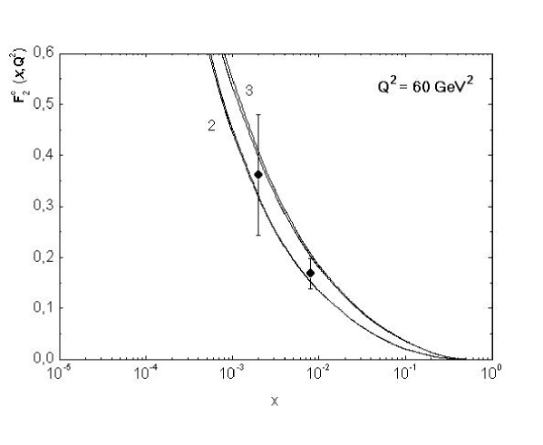
Figure 4: The structure function $F_{2}^{c}(x,Q^{2})$ as a function of $x$ at $Q^{2}=60$ GeV² compared to ZEUS data [4]. Curves 2 and 3 correspond to RS (at $Q_{0}^{2}=4$ GeV²) [27] and BFKL (at $Q_{0}^{2}=1$ GeV²) [28] parametrizations obtained with our off mass shell matrix and ones from Ref. [25].

The ranges of integration correspond to the requirement of positive values in the arguments of the square roots in Eqs. (23), (24), (33) and (34) and also obey to the kinematical restriction $(z\equiv x/y)\leq z_{0}$ with $z_{0}$ from Eq. (22).

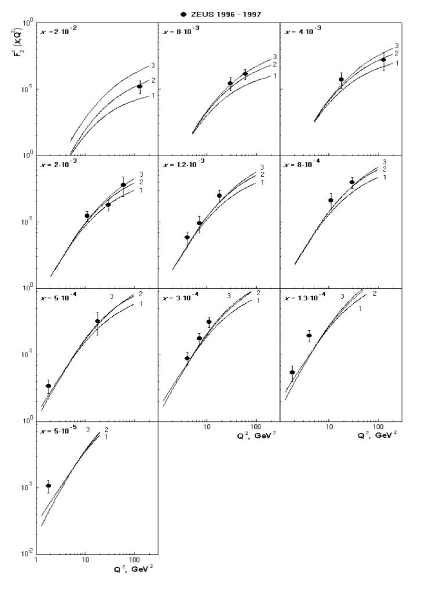
Figure 5: The structure function $F_{2}^{c}(x,Q^{2})$ as a function of $Q^{2}$ for different values of $x$ compared to ZEUS data [4]. Curves 1, 2 and 3 are as in Fig. 2.

In Figs. 2 and 3 we show the SF $F_{2}^{c}$ as a function $x$ for different values of $Q^{2}$ in comparison with ZEUS [4] and H1 [5] experimental data. For comparison we present the results of the calculation with two different parametrizations for the unintegrated gluon distribution $\Phi(x,k^{2}_{\bot},Q_{0}^{2})$ in the forms given by Eq. (41)  and Eq. (43) at $Q_{0}^{2}=4$ GeV².

The differences observed between the curves 2 and 3 are due to the different behaviour of the unintegrated gluon distribution as function $x$ and $k_{\bot}$.

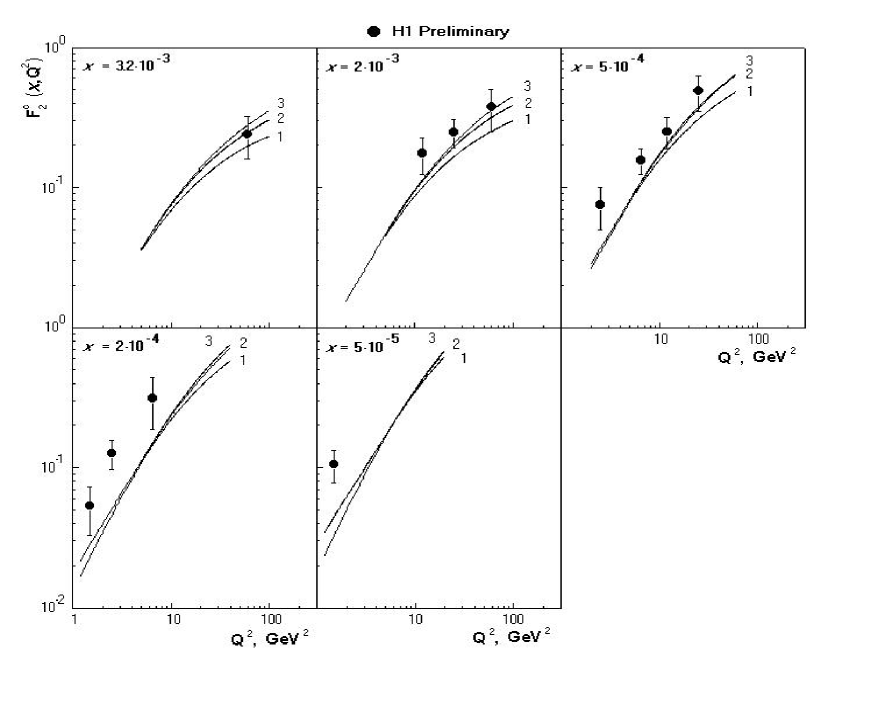
Figure 6: The structure function $F_{2}^{c}(x,Q^{2})$ as a function of $Q^{2}$ for different values of $x$ compared to H1 data [5]. Curves 1, 2 and 3 are as in Fig. 2.

We see that at large $Q^{2}$ ($Q^{2}\geq 10$ GeV²) the SF $F_{2}^{c}$ obtained in the $k_{T}$ factorization approach is higher than the SF obtained in the standard parton model with the GRV gluon density at the LO approximation (see curve 1) and has a more rapid growth in comparison with the standard parton model results, especially at $Q^{2}\sim 130$ GeV² [38]. At $Q^{2}\leq 10$ GeV² the predictions from perturbative QCD (in GRV approach) and those based on the $k_{T}$ factorization approach are very similar and show the disagreement with data below $Q^{2}=7$ GeV² . Unfortunately the available experimental data do not permit yet to distinguish the $k_{T}$ factorization effects from those due to boundary conditions [27].

Fig. 4 shows the structure function $F_{2}^{c}$ at $Q^{2}=60$ GeV² obtained with two different gluon densities, i.e. RS (at $Q_{0}^{2}=4$ GeV²) and BFKL (at $Q_{0}^{2}=1$ GeV²) parametrizations. The difference between curves 2 and 3 are mainly due to the different $Q_{0}^{2}$ value used (as we have already shown in Figs. 2 and 3, the difference due to the parametrizations is essentially smaller). From Figs. 2, 3 and 4, we note that the difference between the $k_{T}$ factorization results and those from perturbative QCD increases when we change the value of $Q_{0}^{2}$ in Eq. (3) from 4 GeV² to 1 GeV² [38]. In addition, for each case presented in Fig. 4. we have done the calculations with our off mass shell matrix elements and those from Ref. [25] . The predictions are very similar and cannot be distinguished on curves 2 and 3.

For completeness, in Figs. 5 and 6 we present the SF $F_{2}^{c}$ as a function $Q^{2}$ for different values of $x$ in comparison with ZEUS [4] and H1 [5] experimental data.

4 Predictions for $F_{L}^{c}$

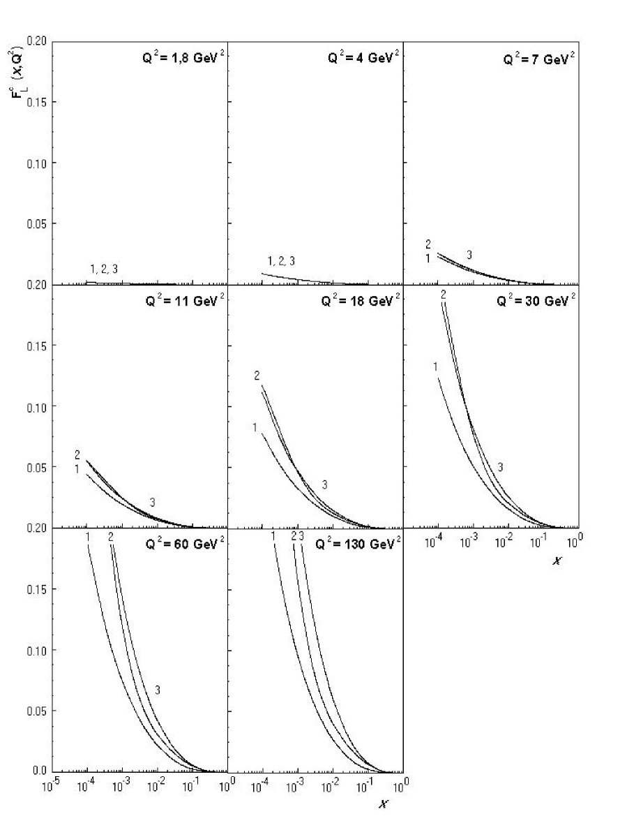
Figure 7: The structure function $F_{L}^{c}(x,Q^{2})$ as a function of $x$ for different values of $Q^{2}$. Curves 1, 2 and 3 are as in Fig. 2.

To calculate the SF $F_{L}^{c}$ we have used Eq. (45) with the replacement of the coefficient function $C_{2}^{g}$ by $C_{L}^{g}$, which is given by Eq. (21).

In Fig. 7 we show the predictions for $F_{L}^{c}$ obtained with different unintegrated gluon distributions. The difference between the results obtained in perturbative QCD and from the $k_{T}$ factorization approach is quite similar to the $F_{2}^{c}$ case discussed above.

The ratio $R^{c}=F_{L}^{c}/F_{2}^{c}$ is shown in Fig. 8. We see $R^{c}\approx 0.1\div 0.3$ in a wide region of $Q^{2}$. The estimation of $R^{c}$ is very close to the results for $R=F_{L}/(F_{2}-F_{L})$ ratio (see Refs. [41]-[44]). We would like to note that these values of $R^{c}$ contradict the estimation obtained in Refs. [4, 5]. The effect of $R^{c}$ on the corresponding differential cross-section should be considered in the extraction of $F_{2}^{c}$ from future more precise measurements.

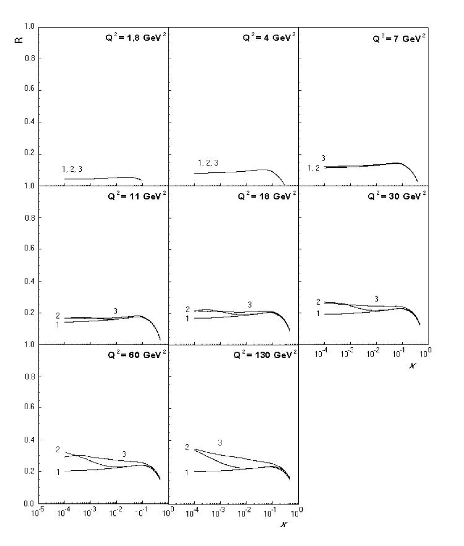
Figure 8: The ratio $R^{c}=F_{L}^{c}(x,Q^{2})/F_{2}^{c}$ as a function of $x$ for different values of $Q^{2}$. Curves 1, 2 and 3 are as in Fig. 2.

For the ratio $R^{c}$ we found quite flat $x$-behavior at low $x$ in the low $Q^{2}$ region (see Fig. 8), where approaches based on perturbative QCD and on $k_{T}$ factorization give similar predictions (see Fig 2, 3, 5, 6 and 7). It is in agreement with the corresponding behaviour of the ratio $R=F_{L}/(F_{2}-F_{L})$ (see Ref. [41]) at quite large values of $\Delta_{P}$ ($\Delta_{P}>0.2-0.3$). The low $x$ rise of $R^{c}$ at high $Q^{2}$ disagrees with early calculations [41] in the framework of perturbative QCD. It could be due to the small $x$ resummation, which is important at high $Q^{2}$ (see Fig 2, 3, 5, 6 and 7). We plan to study in future this effect on $R$ in the framework of $k_{T}$ factorization.

5 Conclusions

We have performed the calculation of the perturbative parts for the structure functions $F_{2}^{c}$ and $F_{L}^{c}$ for a gluon target having nonzero momentum squared, in the process of photon-gluon fusion. The results have quite compact form for both: the Feynman gauge and a nonsense (or BFKL-like) gluon polarizations.

We have applied the results in the framework of $k_{T}$ factorization approach to the analysis of present data for the charm contribution to $F_{2}$ ($F_{2}^{c}$) and we have given the predictions for $F_{L}^{c}$. The analysis has been performed with several parametrizations of unintegrated gluon distributions (RS and BFKL) for comparison. We have found good agreement of our results, obtained with RS and BFKL parametrizations of unintegrated gluons distributions at $Q_{0}^{2}=4$ GeV², with experimental $F_{2}^{c}$ HERA data, except at low $Q^{2}$ ($Q^{2}\leq 7$ GeV²) . We have also obtained quite large contribution of the SF $F_{L}^{c}$ at low $x$ and high $Q^{2}$ ($Q^{2}\geq 30$ GeV²).

We would like to note the good agreement between our results for $F_{2}^{c}$ and the ones obtained in Ref. [46] by Monte-Carlo studies. Moreover, we have also good agreement with fits of H1 and ZEUS data for $F_{2}^{c}$ (see recent reviews in Ref. [47] and references therein) based on perturbative QCD calculations at NLO. But unlike to these fits, our analysis uses universal unintegrated gluon distribution, which gives in the simplest way the main contribution to the cross-section in the high-energy limit.

It could be also very useful to evaluate the complete $F_{2}$ itself and the derivatives of $F_{2}$ with respect to the logarithms of $1/x$ and $Q^{2}$ with our expressions using the unintegrated gluons. We are considering to present this work and also the predictions for $F_{L}$ in a forthcoming article.

The consideration of the SF $F_{2}$ in the framework of the leading-twist approximation of perturbative QCD (i.e. for “pure” perturbative QCD) leads to very good agreement (see Ref. [39] and references therein) with HERA data at low $x$ and $Q^{2}\geq 1.5$ GeV². The agreement improves at lower $Q^{2}$ when higher twist terms are taken into account [40]. As it has been studied in Refs. [39, 40], the SF $F_{2}$ at low $Q^{2}$ is sensitive to the small-$x$ behavior of quark distributions. Thus, the analysis of $F_{2}$ in a broader $Q^{2}$ range should require the incorporation of parametrizations for unintegrated quark densities, introduced recently (see Ref. [48] and references therein).

The study of the complete SF $F_{L}$ should also be very interesting. The structure function $F_{L}$ depends strongly on the gluon distribution (see, for example, Ref. [49]), which in turn is determined [50] by the derivative $dF_{2}/dlnQ^{2}$. Thus, in the framework of perturbative QCD at low $x$ the relation between $F_{L}$, $F_{2}$ and $dF_{2}/dlnQ^{2}$ could be violated by non-perturbative contributions, which are expected to be important in the $F_{L}$ case (see Ref. [51]). The application of present analysis to $F_{L}$ will give a “non pure” perturbative QCD predictions for the structure function that should be compared with data [42, 44] and with the “pure” perturbative results of Ref. [41].

Acknowledgments

We are grateful to Profs. V.S. Fadin, M. Ciafaloni, I.P. Ginzburg, H. Jung, E.A. Kuraev, L.N. Lipatov and G. Ridolfi for useful discussions. N.P.Z. thanks S.P. Baranov for a careful reading of the manuscript and useful remarks. We thank also to participants of the Workshop “Small $x$ phenomenology” (Lund, March 2001) for the interest in this work and discussions.

One of the authors (A.V.K.) was supported in part by Alexander von Humboldt fellowship and INTAS grant N366. G.P. acknowledges the support of Xunta de Galicia (PGIDT00 PX20615PR) and CICyT (AEN99-0589-C02-02). N.P.Z. also acknowledge the support of Royal Swedish Academy of Sciences.

A Appendix

Here we present the contribution to the amplitude of the DIS process from scalar diagrams in the elastic forward scattering of a photon on a parton. In analogy to Eq. (6) one can represent any one-loop diagram of the elastic forward scattering

$$D_{m_{1}m_{2}m_{3}m_{4}}\equiv\int\frac{d^{D}k_{1}}{{(2\pi)}^{D/2}}\,d^{m_{1}}(k_{1})\,d^{m_{2}}(k-k_{1})\,d^{m_{3}}(q+k_{1})\,d^{m_{4}}(q+k_{1}-k),$$ (A.1)

where $d(k)=(k^{2}-m^{2})^{-1}$, in the form :

$$D_{m_{1}m_{2}m_{3}m_{4}}~{}=~{}\sum_{n=0}^{\infty}{\biggl{(}\frac{1}{x}\biggr{)}}^{n}\tilde{k}(n)\;\int_{0}^{1/(1+4a+b)}dz~{}z^{n-1}\beta(z)\tilde{f}_{m_{1}m_{2}m_{3}m_{4}}(z),$$ (A.2)

For application of Eqs. (A.1) and (A.2) to $F_{2}$ and $F_{L}$ coefficient functions, only even $n$ are needed. We choose $\tilde{k}(n)$ so that $\tilde{k}(2n)=1$.

Below we rewrite Eq. (A.2) in the symbolic form:

$$D_{m_{1}m_{2}m_{3}m_{4}}~{}\longrightarrow~{}\tilde{k}(n),~{}\tilde{f}_{m_{1}m_{2}m_{3}m_{4}}(z)$$ (A.3)

Then, we can represent the needed formulae by:

1. The loops:

$$D_{0110} \longrightarrow \tilde{k}(n)=1,~{}~{}~{}~{}~{}~{}~{}~{}\tilde{f}_{0110}(z)=1,$$

$$D_{1001} \longrightarrow \tilde{k}(n)=(-1)^{n},~{}~{}\tilde{f}_{1001}(z)=1$$ (A.4)

2. The triangles:

$$D_{1110} = D_{0111}~{}\longrightarrow~{}\tilde{k}(n)=1,~{}~{}~{}~{}~{}~{}~{}~{}\tilde{f}_{1110}(z)=\tilde{f}_{0111}(z)=-z\;f_{1}(z)$$

$$D_{1011} = D_{1101}~{}\longrightarrow~{}\tilde{k}(n)=(-1)^{n},~{}~{}\tilde{f}_{1011}(z)=\tilde{f}_{1101}(z)=-z\;f_{1}(z)$$ (A.5)

3. The boxes:

$$D_{2110} \longrightarrow \tilde{k}(n)=1,~{}~{}~{}~{}~{}~{}~{}~{}~{}~{}~{}~{}~{}~{}~{}~{}~{}\tilde{f}_{0110}(z)=-4z^{2}\;f_{2}(z)$$ (A.6)

$$D_{1111} \longrightarrow \tilde{k}(n)=\frac{(1+(-1)^{n})}{2},~{}~{}\tilde{f}_{1111}(z)=4z^{2}\;f_{1}(z)$$ (A.7)

We would like to note that the result for the second box $D_{1111}$ is very similar to ones for the triangles. In the case of massless quarks this property has been observed in Refs. [18, 52].

B Appendix

We compare the results obtained in Sect. 2 and Appendix A with well known formulae obtained in earlier works (see Refs. [16, 17]).

Following Ref. [17] let us consider the kinematics of virtual $\gamma\gamma$ forward scattering. According to the optical theorem (see Sect. 1) the quantity $F^{\mu\nu\alpha\beta}$ is the absorptive part of the $\gamma\gamma$ forward amplitude, connected with the cross section in the usual way. (The expression of the amplitude in terms of the electromagnetic currents is given in Sect. 1).

In the expansion of $F^{\mu\nu\alpha\beta}$ into invariant functions one should take into account Lorentz invariance, $T$-invariance (symmetry in the substitution $\mu\nu\leftrightarrow\alpha\beta$) and gauge invariance as well, i.e.

$$q_{1}^{\mu}F^{\mu\nu\alpha\beta}=q_{1}^{\nu}F^{\mu\nu\alpha\beta}=q_{2}^{\alpha}F^{\mu\nu\alpha\beta}=q_{2}^{\beta}F^{\mu\nu\alpha\beta}$$ (B.1)

The tensors in which $F^{\mu\nu\alpha\beta}$ is expanded can be constructed in terms of vectors $q_{1}^{\mu}$, $q_{2}^{\mu}$ and the tensor $g^{\mu\nu}$. In order to take into account explicitly gauge invariance, it is convenient to use their linear combinations:

$${\cal Q}_{1}^{\mu} = \sqrt{\frac{-q_{1}^{2}}{{\cal X}}}\biggl{[}q_{2}^{\mu}-q_{1}^{\mu}\frac{(q_{1}q_{2})}{q_{1}^{2}}\biggr{]},~{}~{}{\cal Q}_{2}^{\mu}~{}=~{}\sqrt{\frac{-q_{2}^{2}}{{\cal X}}}\biggl{[}q_{1}^{\mu}-q_{2}^{\mu}\frac{(q_{1}q_{2})}{q_{2}^{2}}\biggr{]},$$ (B.2)

$$R^{\mu\nu} = R^{\nu\mu}~{}=~{}-g^{\mu\nu}+{{\cal X}}^{-1}\biggl{[}(q_{1}q_{2})(q_{1}^{\mu}q_{2}^{\nu}+q_{1}^{\nu}q_{2}^{\mu})-q_{1}^{2}q_{2}^{\mu}q_{2}^{\nu}-q_{2}^{2}q_{1}^{\mu}q_{1}^{\nu}\biggr{]},$$ (B.3)

where

$${\cal X}=(q_{1}q_{2})^{2}-q_{1}^{2}-q_{2}^{2}$$ (B.4)

The unit vectors ${\cal Q}_{i}^{\mu}$ are orthogonal to the vectors $q_{i}^{\mu}$ and the symmetrical tensor $R^{\mu\nu}$ is orthogonal both to $q_{1}^{\mu}$ and $q_{2}^{\mu}$, i.e. to ${\cal Q}_{1}^{\mu}$ and ${\cal Q}_{2}^{\mu}$:

$$q_{1}^{\mu}{\cal Q}_{1}^{\mu}=q_{2}^{\mu}{\cal Q}_{2}^{\mu}=0,~{}~{}q_{i}^{\mu}R^{\mu\nu}={\cal Q}_{i}^{\mu}R^{\mu\nu}=0,$$

$${\cal Q}_{1}^{2}={\cal Q}_{1}^{2}=1,~{}~{}R^{\mu\nu}R^{\mu\nu}=2,~{}~{}R^{\mu\nu}R^{\nu\rho}=-R^{\mu\rho}$$ (B.5)

We note, that $R^{\mu\nu}$ is a metric tensor of a subspace which is orthogonal to $q_{1}^{\mu}$ and $q_{2}^{\mu}$. In the c.m.s. of the photons, only two components of $R^{\mu\nu}$ are different from 0 ($R^{xx}=R^{yy}=1$).

The choice of independent tensors in which the expansion is carried out, has a high degree of arbitrariness. We make this choice so that these tensors are orthogonal to each other, and the invariant functions have a simple physical interpretation:

$$F^{\mu\nu\alpha\beta} = R^{\mu\alpha}R^{\nu\beta}F_{TT}+R^{\mu\alpha}{\cal Q}_{2}^{\nu}{\cal Q}_{2}^{\beta}F_{TS}+{\cal Q}_{1}^{\mu}{\cal Q}_{1}^{\alpha}R^{\nu\beta}F_{ST}$$

$$+ {\cal Q}_{1}^{\mu}{\cal Q}_{1}^{\alpha}{\cal Q}_{2}^{\nu}{\cal Q}_{2}^{\beta}F_{SS}+\frac{1}{2}\biggl{[}R^{\mu\nu}R^{\alpha\beta}+R^{\mu\beta}R^{\nu\alpha}-R^{\mu\alpha}R^{\nu\beta}\biggr{]}F_{TT}^{\tau}$$

$$- \biggl{[}R^{\mu\nu}{\cal Q}_{1}^{\alpha}{\cal Q}_{2}^{\beta}+R^{\mu\beta}{\cal Q}_{1}^{\alpha}{\cal Q}_{2}^{\nu}+(\mu\nu\leftrightarrow\alpha\beta)\biggr{]}F_{TS}^{\tau}$$

$$+ \biggl{[}R^{\mu\nu}R^{\alpha\beta}-R^{\mu\beta}R^{\nu\alpha}\biggr{]}F_{TT}^{a}-\biggl{[}R^{\mu\nu}{\cal Q}_{1}^{\alpha}{\cal Q}_{2}^{\beta}-R^{\mu\beta}{\cal Q}_{1}^{\alpha}{\cal Q}_{2}^{\nu}+(\mu\nu\leftrightarrow\alpha\beta)\biggr{]}F_{TS}^{a}$$

The dimensionless invariant functions $F_{ab}$ defined here only depend on the invariants $W^{2}=(q_{1}+q_{2})^{2}$, $q_{1}^{2}$ and $q_{2}^{2}$. The first four functions are expressed through the cross sections $\sigma_{ab}$ ($a,b\equiv S,T$ for scalar and transverse photons, respectively). The amplitudes $F_{ab}^{\tau}$ correspond to transitions with spin-flip for each of the photons with total helicity conservation. The last two amplitudes are antisymmetric.

We would like to represent the results of Ref. [16] in terms of our functions, introduced in Section 2.

First of all, we return to the variables introduced in Sect. 2. Then, we have

$${\cal X}~{}=~{}\frac{Q^{4}}{4x^{2}}\,\tilde{\beta}^{2},~{}~{}{\cal Q}_{1}^{\mu}~{}=~{}\sqrt{\frac{4bx^{2}}{Q^{2}\tilde{\beta}^{2}}}\biggl{[}q_{2}^{\mu}+\frac{1}{2bx}q_{1}^{\mu}\biggr{]},~{}~{}{\cal Q}_{2}^{\mu}~{}=~{}\sqrt{\frac{4bx^{2}}{Q^{2}\tilde{\beta}^{2}}}\biggl{[}q_{1}^{\mu}+\frac{1}{2x}q_{2}^{\mu}\biggr{]},$$ (B.7)

The results of Ref. [16] have the form :

$$\tilde{\beta}F_{TT} = 4x\beta\biggl{[}1+4(a-1-b)T+12bT^{2}-\biggl{\{}1-8a^{2}x^{2}+2(2a-1-b$$

$$+2bx(1-x(1+b)))T+24b^{2}T^{2}\biggr{\}}f_{1}+bx^{2}f_{2}\biggr{]},$$

$$\tilde{\beta}F_{TS} = -16x\beta\biggl{[}T-2x\biggl{\{}ax-b(1+2x(a-1-b))T-6b^{2}T^{2}\biggr{\}}f_{1}$$

$$+bx^{2}(6a-b+6bT)Tf_{2}\biggr{]},$$

$$\tilde{\beta}F_{ST} = -16x\beta\biggl{[}T-2x\biggl{\{}ax-(1+x(2a-1-b))T-6b^{2}T^{2}\biggr{\}}f_{1}$$

$$+x^{2}(6a-b+6bT)Tf_{2}\biggr{]},$$

$$\tilde{\beta}F_{SS} = 64bxT^{2}\beta\biggl{[}2-(1+2bx^{2})f_{1}-bx^{2}f_{2}\biggr{]},$$

$$\tilde{\beta}F_{TT}^{\tau} = 8x\beta\biggl{[}2aT+(1-a^{2})\frac{x^{2}}{\tilde{\beta}^{2}}+6bT^{2}+x^{2}\biggl{\{}2(1+a+b)-b-2b(2a-1-b)T$$

$$-12b^{2}T^{2}\biggr{\}}f_{1}\biggr{]},$$

$$\tilde{\beta}F_{TS}^{\tau} = \tilde{\beta}F_{ST}^{\tau}~{}=~{}16b^{1/2}xT\beta\biggl{[}2x-3T+x^{2}\biggl{\{}2a-1-b+6bT\biggr{\}}f_{1}\biggr{]},$$

$$\tilde{\beta}F_{TT}^{a} = 4\beta\biggl{[}x-4T+\biggl{\{}2T-x\biggr{\}}f_{1}-bx^{3}f_{2}\biggr{]},$$

$$\tilde{\beta}F_{TS}^{a} = \tilde{\beta}F_{ST}^{a}~{}=~{}-16b^{3/2}x^{2}T\beta\biggl{[}2f_{1}-f_{2}\biggr{]},$$

where

$$T=\frac{x(1-x(1+b))}{\tilde{\beta}^{2}}$$

Doing the needed projections on Eqs. (B) we can express the above functions as combinations of $f^{(1)},~{}f^{(2)},~{}\tilde{f}^{(1)}$ and $\tilde{f}^{(2)}$ (see Sect. 2).

$$\tilde{\beta}^{2}F_{SS} = f^{(1)},~{}~{}~{}~{}~{}\tilde{\beta}^{2}F_{ST}~{}=~{}\tilde{\beta}^{2}f^{(1)}+\frac{1}{2}f^{(2)}$$

$$\tilde{\beta}^{2}F_{TS} = \frac{1}{2}\biggl{[}\tilde{f}^{(2)}-f^{(2)}\biggr{]},~{}~{}~{}~{}~{}\tilde{\beta}^{2}F_{TT}~{}=~{}\frac{1}{2}\biggl{[}\tilde{\beta}^{2}\tilde{f}^{(1)}-f^{(1)}\biggr{]}$$ (B.8)

The coefficient functions calculated in Sect. 2 can be expressed as combinations of $F_{AB}~{}~{}(A,B=S,T)$.

For non interacting gluons:

$$\tilde{\beta}^{2}C_{2} = {\cal K}\;\Biggl{[}F_{SS}+F_{ST}-2(F_{TT}+F_{TS})\Biggr{]},$$

$$\tilde{\beta}^{2}C_{L} = {\cal K}\;\Biggl{[}F_{SS}-2F_{TS}+4bx^{2}\Bigl{(}F_{ST}-2F_{TT}\Bigr{)}\Biggr{]}$$ (B.9)

For the BFKL projector:

$$\tilde{\beta}^{4}C_{2,BFKL} = {\cal K}\;\Biggl{[}F_{SS}+F_{ST}+F_{TS}+F_{TT}\Biggr{]},$$

$$\tilde{\beta}^{4}C_{L,BFKL} = {\cal K}\;\Biggl{[}F_{SS}+F_{TS}+4bx^{2}\Bigl{(}F_{ST}+F_{TT}\Bigr{)}\Biggr{]}$$ (B.10)

C Appendix

Here we consider the particular cases: $k^{2}=0$, $m^{2}=0$ and $Q^{2}\to 0$ which are relevant to compare with others.

C.1 The case $k^{2}=0$

When $k^{2}=0$

$$C^{g}_{2}(x)~{}=~{}{\cal K}\;\left[f^{(1)}+\frac{3}{2}\;f^{(2)}\right]~{}~{}~{}\mbox{ and }~{}~{}~{}C^{g}_{L}(x)~{}=~{}{\cal K}\;f^{(2)}$$ (C.1)

with

$$f^{(1)} = -2\;\beta\Biggl{[}\biggl{(}1-2x(1-x)(1-2a)\biggr{)}-\biggl{(}1-2x(1-2a)+2x^{2}(1-4a^{2})\biggr{)}$$ (C.2)

$$\;L(\beta)\Biggr{]}$$

$$f^{(2)} = 8x\;\beta\Biggl{[}(1-x)-2xa\;L(\beta)\Biggr{]},$$ (C.3)

where

$$\beta^{2}=1-\frac{4ax}{(1-x)}$$

and the function $L(\beta)$ has been defined in Eq. (36).

Equations (C.1)-(C.3) coincide with the results of Ref. [54].

Indeed, we have

$$C^{g}_{2} = {\cal K}\;(-2)\beta\Biggl{[}\biggl{(}1-4x(2-a)(1-x)\biggr{)}$$ (C.4)

$$- \biggl{(}1-2x(1-2a)+2x^{2}(1-6a-4a^{2})\biggr{)}\;L(\beta)\Biggr{]}$$

$$C^{g}_{L} = {\cal K}\;8x\beta\Biggl{[}(1-x)-2xa\;L(\beta)\Biggr{]}$$ (C.5)

The consideration of the BFKL projector does not change the results given above because the additional terms (see Eq. (31)) are proportional to $k^{2}$ and they are negligible. The expression in Eq. (C.5) also coincides with the corresponding result in Ref. [26] (see Eqs. (A17,A18)).

C.2 The case $m^{2}=0$

When $m^{2}=0$ the coefficient functions $C^{g}_{k}(x)$ are defined through $f^{(1)}$ and $f^{(2)}$ (see Eqs. (20), (21)) being in this case

$$f^{(1)} = -2\Biggl{[}2-\biggl{(}1-2x(1+b)+2x^{2}(1+b)^{2}\biggr{)}\;L(\tilde{\beta})\Biggr{]}$$ (C.6)

$$f^{(2)} = 8x(1+b)(1-(1+b)x)\Biggl{[}1-2bx^{2}\;L(\tilde{\beta})\Biggr{]}$$ (C.7)

For the coefficient functions themselves, we have

$$\tilde{\beta}^{4}\;C^{g}_{2} = {\cal K}\;(-2)\left(1-x(1+b)\right)\Biggl{[}2\biggl{(}1-2x(1+b)+\frac{x^{2}(1-b)^{2}}{1-x(1+b)}\biggr{)}$$ (C.8)

$$- \biggl{(}1-x(1+b)-4x^{3}b(1+b)+\frac{x^{2}(1-b)^{2}}{1-x(1+b)}\biggr{)}\;L(\tilde{\beta})\Biggr{]}$$

$$\tilde{\beta}^{4}\;C^{g}_{L} = {\cal K}\;8x\left(1-x(1+b)\right)\Biggl{[}\biggl{(}(1+b)-2bx\biggl{[}1+\frac{x^{2}(1-b)^{2}}{1-x(1+b)}\biggr{]}\biggr{)}$$ (C.9)

$$+ bx\biggl{(}1-3x(1+b)+4x^{3}b(1+b)+\frac{x^{2}(1-b)^{2}}{1-x(1+b)}\biggr{)}\;L(\tilde{\beta})\Biggr{]}$$

In the case of the BFKL projector, the coefficient functions $C^{g}_{k}(x)$ are defined by Eqs. (C.1), (23) and (24) with the replacement $f^{(i)}\to f^{(i)}_{BFKL}$ as in Eq. (32). In Eq. (32) the expressions for $f^{(i)}$ can be found in Eqs. (C.6), (C.7) while for $\tilde{f}^{(i)}$ are given by:

$$\tilde{f}^{(1)} = -\frac{(1+b)(1-x(1+b))}{bx}\Biggl{[}1-2bx^{2}\;L(\tilde{\beta})\Biggr{]}=-\frac{1}{8bx^{2}}f^{(2)}$$ (C.10)

$$\tilde{f}^{(2)} = 4(1-x(1+b))^{2}\Biggl{[}3-(1+2bx^{2})\;L(\tilde{\beta})\Biggr{]}$$ (C.11)

and, thus,

$$f^{(1)}_{BFKL} = C^{g}_{2}/{\cal K}$$ (C.12)

$$\tilde{\beta}^{4}\;f^{(2)}_{BFKL} = 8x(1-x(1+b))\Biggl{[}1+b-18bx(1-x(1+b))$$ (C.13)

$$+ 2bx\left(3-4x(1+b)+6bx^{2}(1-x(1+b))\right)\;L(\tilde{\beta})\Biggr{]}$$

For the coefficient functions $C^{g}_{k,BFKL}(x)$ we have the following results:

$$\tilde{\beta}^{8}\;C^{g}_{2,BFKL} = {\cal K}\;(-2)\left(1-x(1+b)\right)\Biggl{[}2\biggl{(}1-5x(1+b)$$ (C.14)

$$+ x^{2}(1+48b+b^{2})+x^{3}(1+b)(1-48b+b^{2})+\frac{x^{4}(1-b)^{4}}{1-x(1+b)}\biggr{)}$$

$$- \biggl{(}1-x(1+b)+(1-30b+b^{2})x^{2}+(1-50b+b^{2})x^{3}(1+b)$$

$$+ 72x^{4}b^{2}-56x^{5}b^{2}(1+b)+\frac{x^{4}(1-b)^{4}}{1-x(1+b)}\biggr{)}\;L(\tilde{\beta})\Biggr{]}$$

$$\tilde{\beta}^{8}\;C^{g}_{L,BFKL} = {\cal K}\;8x\left(1-x(1+b)\right)\Biggl{[}\biggl{(}(1+b)-20bx+24b(1+b)x^{2}$$ (C.15)

$$- 2b(1+12b+b^{2})x^{3}-2(1+b)b(1-12b+b^{2})x^{4}-2bx\;\frac{x^{4}(1-b)^{4}}{1-x(1+b)}\biggr{)}$$

$$+ bx\biggl{(}7-11x(1+b)+(1-42b+b^{2})x^{2}+(1-30b+b^{2})(1+b)x^{3}$$

$$+ 24b^{2}x^{4}-8b^{2}(1+b)x^{5}+\frac{x^{4}(1-b)^{4}}{1-x(1+b)}\biggr{)}\;L(\tilde{\beta})\Biggr{]}$$

C.3 The case $Q^{2}\to 0$

Using the definitions in Eq. (35), when $x\to 0$ we have got the following relations (at $O(x)$):

for the intermediate functions:

$$\tilde{\beta}^{2} = 1-4x\Delta,~{}~{}\beta^{2}=\hat{\beta}^{2}(1-4\gamma x),$$

$$f_{1} = L(\hat{\beta})\left(1+2x(\gamma+\Delta)\right)-2x(\gamma+\Delta)\frac{(1-\Delta)}{z},~{}~{}$$

$$f_{2} = -\frac{2(1-\Delta)}{z}\biggl{[}1-2x\frac{1-\Delta-2z}{z}\;(\gamma+\Delta)\biggr{]},$$ (C.16)

where

$$z=\frac{\rho}{2},~{}~{}~{}\gamma=\frac{z/2}{(1-\Delta)(1-\Delta-2z)}$$

for the basic functions:

$$f^{(1)} = -2\hat{\beta}\Biggl{[}1-2(1-\Delta)(\Delta-z)-\Bigl{(}1-2(1-\Delta)\Delta+2(1-z)z\Bigr{)}L(\hat{\beta})$$ (C.17)

$$+ 2x\Biggl{\{}\frac{1-\Delta}{z}\left(\Delta+(\Delta-z)(1-2z\Delta)\right)-\frac{1-\Delta-z}{z}\,\gamma$$

$$+ \biggl{(}1-\Delta\Bigl{[}3-2(1-\Delta)\Delta+2(1-z)z\Bigr{]}\biggr{)}L(\hat{\beta})\Biggr{\}}\Biggr{]},$$

$$f^{(2)} = 8x\hat{\beta}\Biggl{[}(1-\Delta)\left(1-2\frac{\Delta(1-\Delta)}{z}(z-\Delta)\right)-\Bigl{(}2\Delta^{2}(1-\Delta)$$

$$+ z(1-2\Delta(1-\Delta))\Bigr{)}L(\hat{\beta})\Biggr{]},$$

$$x\tilde{f}^{(1)} = -\hat{\beta}\Biggl{[}\biggl{\{}(1-\Delta)-x(3-6\Delta+4\Delta^{2})\biggr{\}}-\biggl{\{}z+2x(\Delta(1-\Delta)-z)\biggr{\}}L(\hat{\beta})\Biggr{]},$$

$$x\tilde{f}^{(2)} = 4x\hat{\beta}(1-\Delta)^{2}\Bigl{[}2-L(\hat{\beta})\Bigr{]},$$ (C.18)

and, thus,

$$f^{(1)}_{BFKL} = f^{(1)}~{}+~{}4\hat{\beta}\Delta\Biggl{[}3\Bigl{(}1-\Delta-zL(\hat{\beta})\Bigr{)}-x\Biggl{\{}11-46\Delta+40\Delta^{2}+4z(1-\Delta)$$ (C.19)

$$- 2\Bigl{[}1-5(1-\Delta)\Delta+z(5-2z-12\Delta)\Bigr{]}\Biggr{\}}L(\hat{\beta})\Biggr{]},$$

$$f^{(2)}_{BFKL} = f^{(2)}~{}-~{}48x\hat{\beta}\Delta(1-\Delta)\Bigl{[}2-L(\hat{\beta})\Bigr{]}.$$ (C.20)

Similarly to Eq. (C.18), the coefficient functions in Eq. (39) and the functions $f^{(1)}_{BFKL}$ in Eq. (40) have the additional terms proportional $x$.

$$C^{g}_{2}/{\cal K} = f^{(1)}~{}+~{}4x\hat{\beta}\Biggl{[}\,6\,\frac{\Delta^{2}(1-\Delta)^{2}}{z}+3-\Delta\Bigl{(}11-16\Delta+10\Delta^{2}+4z(1-\Delta)\Bigr{)}$$ (C.21)

$$+ \Biggl{\{}2\Delta\Bigl{[}1-5(1-\Delta)\Delta+z(5-2z-3\Delta)\Bigr{]}-3z\Biggr{\}}L(\hat{\beta})\Biggr{]},$$

$$C^{g}_{L}/{\cal K} = 8x\hat{\beta}\Biggl{[}\,2\,\frac{\Delta^{2}(1-\Delta)^{2}}{z}+1-2\Delta\Bigl{(}2-3\Delta+2\Delta^{2}+z(1-\Delta)\Bigr{)}$$ (C.22)

$$+ \Biggl{\{}\Delta\Bigl{[}1-4(1-\Delta)\Delta+2z(2-z-\Delta)\Bigr{]}-z\Biggr{\}}L(\hat{\beta})\Biggr{]},$$

$$C^{g}_{2,BFKL}/{\cal K} = C^{g}_{2}/{\cal K}~{}+~{}4\hat{\beta}\Delta\Biggl{[}3\Bigl{(}1-\Delta-zL(\hat{\beta})\Bigr{)}-x\Biggl{\{}47-130\Delta+88\Delta^{2}$$ (C.23)

$$+ 4z(1-\Delta)-2\Bigl{[}10-23\Delta+14\Delta^{2}+z(5-2z-18\Delta)\Bigr{]}L(\hat{\beta})\Biggr{\}}\Biggr{]},$$

$$C^{g}_{L,BFKL}/{\cal K} = C^{g}_{L}/{\cal K}~{}-~{}48x\hat{\beta}\Delta\Biggl{[}(1-\Delta)(2-3\Delta)-\Bigl{[}(1-\Delta)^{2}-z\Delta\Bigr{]}L(\hat{\beta})\Biggr{]}$$ (C.24)

References

- [1]
- [2] H1 Collab.: S. Aid et al., Z. Phys. C72 (1996) 593; Nucl. Phys. B545 (1999) 21.
- [3] ZEUS Collab.: J. Breitweg et al., Phys. Lett. B407 (1997)402.
- [4] ZEUS Collab.: J. Breitweg et al., Eur. Phys. J. C12 (2000) 35.
- [5] H1 Collab.: S. Adloff et al., Paper submitted to ICHEP2000, Osaka, Japan, Abstract 984.
- [6] EM Collab.: J.J. Aubert et al., Nucl. Phys. B213 (1983) 31; Phys. Lett. B94 (1980) 96; B110 (1983) 72.
- [7] A.M. Cooper-Sarkar, R.C.E. Devenish and A. De Roeck, Int. J. Mod. Phys. A13 (1998) 3385.
- [8] V.N. Gribov and L.N. Lipatov, Sov. J. Nucl. Phys. 18 (1972) 438, 675.
-
[9]
L.N. Lipatov, Sov. J. Nucl. Phys. 20
(1975) 93;
G. Altarelli and G. Parisi, Nucl. Phys. B126 (1977) 298;
Yu.L. Dokshitzer, Sov. Phys. JETP 46 (1977) 641. -
[10]
B.A. Kniehl et al.,
Z. Phys. C76 (1997) 689;
J. Binnewies et al., Z. Phys. C76 (1997) 677;
M. Cacciari et al., Phys. Rev. D55 (1997) 2736, 7134. - [11] S. Frixione et al., Phys. Lett. B348 (1995) 653, Nucl. Phys. B454 (1995) 3.
- [12] M.A.G. Aivazis et al., Phys. Rev. D50 (1994) 3102.
-
[13]
L.N. Lipatov, Sov. J. Nucl. Phys.
23 (1976) 642;
E.A. Kuraev, L.N. Lipatov and V.S. Fadin, Sov. Phys. JETP 44 (1976) 45, 45 (1977) 199;
Ya.Ya. Balitzki and L.N. Lipatov, Sov. J. Nucl. Phys. 28 (1978) 822;
L.N. Lipatov, Sov. Phys. JETP 63 (1986) 904. - [14] J. Kwiecinski, Acta Phys. Polon. B27 (1996) 3455.
-
[15]
A. V. Lipatov and N.P. Zotov, Mod. Phys. Lett.
A15 (2000) 695;
A. V. Lipatov, V.A. Saleev and N.P. Zotov, Mod. Phys. Lett. A15 (2000) 1727. -
[16]
V.N. Baier, V.S. Fadin and V.A. Khose,
JETP 50 (1966) 156 (in Russian);
V.N. Baier, V.M. Katkov and V.S. Fadin, Relativistic electron radiation, (Moscow, Atomizdat, 1973) (in Russian);
V.G. Zima, Yad. Fiz. 16 (1972) 1051. - [17] V.M. Budnev, I.F. Ginsburg, G.V. Meledin and V.G. Serbo, Phys. Rept. 15 (1975) 181.
- [18] D.I. Kazakov and A.V. Kotikov, Theor.Math.Phys. 73 (1987) 1264; Nucl.Phys. B307 (1988) 721; E: B345 (1990) 299.
- [19] R.K. Ellis, W. Furmanski, and R. Petronzio, Nucl. Phys. B207 (1982) 1; B212 (1983) 29.
- [20] S. Catani, M. Ciafaloni and F. Hautmann, Phys. Lett. B242 (1990) 97; Nucl. Phys. B366 (1991) 135.
- [21] J.C. Collins and R.K. Ellis, Nucl. Phys. B360 (1991) 3.
- [22] E.M. Levin, M.G. Ryskin, Yu.M. Shabelskii and A.G. Shuvaev, Sov. J. Nucl. Phys. 53 (1991) 657.
- [23] E.A. Kuraev and L.N. Lipatov, Sov. J. Nucl. Phys. 16 (1973) 584.
-
[24]
W. Vogelsang,
Z. Phys. C50 (1991) 275;
A. Gabrieli and G. Ridolfi, Phys. Lett. B417 (1998) 369. - [25] G. Bottazzi, G. Marchesini, G.P. Salam, and M. Scorletti, JHEP 9812 (1998) 011.
- [26] S. Catani, M. Ciafaloni, and F. Hautmann, Preprint CERN - TH.6398/92, in Proceeding of the Workshop on Physics at HERA (Hamburg, 1991), v.2, p.690.
- [27] M.G. Ryskin and Yu.M. Shabelski, Z. Phys. C61 (1994) 517; C66 (1995) 151.
- [28] J. Blumlein, Preprint DESY 95-121 (hep-ph/9506203).
- [29] M. Gluck, E. Reya, and A. Vogt, Z. Phys. C67 (1995) 433.
-
[30]
V.N. Fadin and L.N. Lipatov, Phys. Lett. B429 (1998) 127;
M. Ciafaloni and G. Camici, Phys. Lett. B430 (1998) 349. - [31] A.V. Kotikov and L.N. Lipatov, Nucl. Phys. B582 (2000) 19.
- [32] D.A. Ross, Phys. Lett B431 (1998) 161.
- [33] G. Salam. JHEP 9807 (1998) 019; Acta Phys.Polon. B30 (1999) 3679
- [34] S.J. Brodsky, V.S. Fadin, V.T. Kim, L.N. Lipatov, and G.B. Pivovarov, JETP Lett. 70 (1999) 155.
- [35] S. P. Baranov and N.P. Zotov, Phys. Lett. B458 (1999) 389.
-
[36]
N.N. Nikolaev and B.G. Zakharov, Phys. Lett B333 (1994) 250;
Phys. Lett B327 (1994) 157;
J. Kwiecinski, A.D. Martin, and P.J. Sutton, Z. Phys. C71 (1996) 585;
B. Andersson, G. Gustafson, H. Kharrazina, and J. Samuelsson, Z. Phys. C71 (1996) 613;
N.N. Nikolaev and V.R. Zoller, in Proc. QCD-2000, Villefranche-sur-Mer, January 2000 (hep-ph/0001084);
B.I. Ermolaev, M. Greco, and S.I. Troyan, Nucl.Phys. B594 (2001) 71. -
[37]
L3 Collaboration, M. Acciarri et al., Phys. Lett. B453 (1999) 333;
M. Kienzle, talk given at the International Symposium on Evolution Equations and Large Order Estimates in QCD, Gatchina, Russia, May,2000. - [38] A.V. Lipatov and N.P. Zotov, in Proc. of the 8th Int. Workshop on Deep Inelastic Scattering, DIS 2000 (2000), World Scientific, p. 157.
- [39] A.V. Kotikov and G. Parente, Nucl. Phys. B549 (1999) 242; Nucl. Phys. (Proc. Suppl.) 99 (2001) 196; in Proc. of the Int. Conference PQFT98 (1998), Dubna (hep-ph/9810223); in Proc. of the 8th Int. Workshop on Deep Inelastic Scattering, DIS 2000 (2000), Liverpool, p. 198 (hep-ph/0006197).
- [40] A.V. Kotikov and G. Parente, in Proc. Int. Seminar Relativistic Nuclear Physics and Quantum Chromodynamics (2000), Dubna (hep-ph/0012299); in Proc. of the 9th Int. Workshop on Deep Inelastic Scattering, DIS 2001 (2001), Bologna (hep-ph/0106175).
-
[41]
A.V. Kotikov, JETP 80 (1995) 979;
A.V. Kotikov and G. Parente, in Proc. Int. Workshop on Deep Inelastic Scattering and Related Phenomena (1996), Rome, p. 237 (hep-ph/9608409); Mod. Phys. Lett. A12 (1997) 963; JETP 85 (1997) 17; hep-ph/9609439. -
[42]
H1 Collab.: S. Aid et al.,
Phys.Lett. B393 (1997) 452;
H1 Collab.: D. Eckstein, in Proc. Int. Workshop on Deep Inelastic Scattering, (2001), Bologna;
H1 Collab.: M.Klein, in Proc. of the 9th Int. Workshop on Deep Inelastic Scattering, DIS 2001 (2001), Bologna. - [43] R.S. Thorne, Phys.Lett. B418 (1998) 371.
-
[44]
CCFR/NuTeV Collab.: U.K. Yang et al.,
in Proc. Int. Conference on High Energy Physics (2000) Osaka, Japan
(hep-ex/0010001);
CCFR/NuTeV Collab.: A. Bodek, in Proc. of the 9th Int. Workshop on Deep Inelastic Scattering, DIS 2001 (2001), Bologna (hep-ex/00105067). -
[45]
S. Keller, M. Miramontes, G. Parente,
J. Sánchez-Guillén, and O.A. Sampayo,
Phys.Lett. B270 (1990) 61;
L.H. Orr and W.J. Stirling, Phys.Rev.Lett. B66 (1991) 1673;
E. Berger and R. Meng, Phys.Lett. B304 (1993) 318;
A.V. Kotikov, JETP Lett. 59 (1994) 1; Phys.Lett. B338 (1994) 349. - [46] H. Jung, Nucl. Phys. (Proc. Suppl.) 79 (1999) 429.
-
[47]
G. Wolf, Preprint DESY 01-058 (hep-ex/0105055);
L. Gladilin and I. Redoldo, to appear in “The THERA Book” (hep-ph/0105126). - [48] M.A. Kimber, A.D. Martin, and M.G. Ryskin, Phys. Rev. D63 (2001) 114027.
-
[49]
A.M. Cooper-Sarkar, G. Ingelman, R.G. Roberts and D.H. Saxon,
Z. Phys. C39 (1988) 281;
A.V. Kotikov, Phys. Atom. Nucl. 57 (1994) 133; Phys. Rev. D49 (1994) 5746. -
[50]
K. Prytz, Phys.Lett. B311 (1993) 286;
A.V. Kotikov, JETP Lett. 59 (1994) 667;
A.V. Kotikov and G. Parente, Phys.Lett. B379 (1996) 195. - [51] J. Bartels, K.Golec-Biernat, and K. Peters, Eur.Phys.J. C17 (2000) 121.
- [52] A.V. Kotikov, Theor.Math.Phys. 78 (1989) 134.
- [53] A.V. Kotikov, Phys.Lett. B254 (1991) 158; B259 (1991) 314; B267 (1991) 123.
-
[54]
E. Witten,
Nucl. Phys. B104 (1976) 445;
M. Gluck and E. Reya, Phys. Lett. B83 (1979) 98;
F.M. Steffens, W. Melnitchouk, and A.W. Thomas, Eur.Phys.J. C11 (1999) 673.