Theory of the Quark-Gluon Plasma

Theory of the Quark-Gluon Plasma

1 Introduction

In spite of what the title might suggest, I shall not try to cover in these lectures all interesting aspects of the theory of the quark-gluon plasma. I shall rather focus on progress made in recent years in understanding the high temperature phase of QCD by using weak coupling techniques. Such techniques go far beyond strict perturbation theory viewed as an expansion in powers of the gauge coupling. In fact such an expansion becomes meaningless as soon as the coupling is not vanishingly small. However, we shall see that a rather simple structure emerges from weak coupling studies, with a characteristic hierarchy of scales and degrees of freedom. The interactions renormalize the properties of these elementary degrees of freedom, but does not destroy the simple picture of the high temperature quark-gluon plasma as a system of weakly interacting quasiparticles. As we shall see at the end of these lectures, this picture is supported by a first principle calculation of the entropy which reproduces accurately lattice data above 2 or 3 times the critical temperature.

Some of the material presented here is borrowed from the recent review Blaizot:2001nr , and complements can also be found in Blaizot1997 ; Blaizot:1996ns ; BIO95 ; Puri94 ; Coree91 . Another perspective on some of the topics discussed here can be found in the lectures by A. Rebhan.

The outline of the lectures is the following. In order to get a first rough picture of the phase diagram of hadronic matter I use the bag model to describe the quark-hadron phase transition: this exercise will give us some familiarity with the thermodynamics of massless, non-interacting, particles. Then I briefly recall some techniques of quantum field theory at finite temperature needed to treat the interactions KB62 ; Abrikosov63 ; Fetter71 ; BR86 ; Kapusta ; LeBellac96 , and introduce the concept of effective theory in a simple case of a scalar field. Then I proceed to an analysis of the various important scales and degrees of freedom of the quark-gluon plasma and focus on the effective theory for the collective modes which develop at the particular momentum scale $gT$, where $g$ is the gauge coupling and $T$ the temperature. A powerful technique to construct the effective theory is based on kinetic equations which govern the dynamics of the hard degrees of freedom. Some of the collective phenomena that are described by this effective theory are briefly mentioned. Then I turn to the calculation of the entropy and show how the information coded in the effective theory can be exploited in (approximately) self-consistent calculations Blaizot:1999ip ; Blaizot:1999ap ; Blaizot:2001fc .

2 The quark-hadron transition in the bag model.

The phase diagram of dense hadronic matter has the expected shape indicated in Fig. 1. There is a low density, low temperature region, corresponding to the world of ordinary hadrons, and a high density, high temperature region, where the dominant degrees of freedom are quarks and gluons. The precise determination of the transition line requires elaborate non perturbative techniques, such as those of lattice gauge theories (see the lectures by F. Karsch). But one can get rough orders of magnitude for the transition temperature and density using a simple model dealing mostly with non-interacting particles Blaizot:1996ns ; Puri94 .

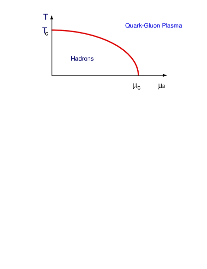
Figure 1: The expected phase diagram of hot and dense hadronic matter in the plane $\left(\mu_{B},T\right)$, where $T$ is the temperature and $\mu_{B}$ the baryon chemical potential

Let us first consider the transition in the case where $\mu_{B}=0$. At low temperature this baryon free matter is composed of the lightest mesons, i.e. mostly the pions. At sufficiently high temperature one should also take into account heavier mesons, but in the present discussion this is an inessential complication. We shall even make a further approximation by treating the pion as a massless particle. At very high temperature, we shall consider that hadronic matter is composed only of quarks and antiquarks (in equal numbers), and gluons, forming a quark-gluon plasma. In both the high temperature and the low temperature phases, interactions are neglected (except for the bag constant to be introduced below). The description of the transition will therefore be dominated by entropy considerations, i.e. by counting the degrees of freedom.

The energy density $\varepsilon$ and the pressure $P$ of a gas of massless pions are given by:

$$\varepsilon=3\cdot{\pi^{2}\over 30}T^{4}\,,\ \ \ \ \ \ P=3\cdot{\pi^{2}\over 90}T^{4},$$ (1)

where the factors 3 account for the 3 types of pions $(\pi^{+},$ $\pi^{-},$ $\pi^{0}).$

The energy density and pressure of the quark-gluon plasma are given by similar formulae:

$$\varepsilon = 37\cdot{\pi^{2}\over 30}T^{4}+B,$$ (2)

$$P = 37\cdot{\pi^{2}\over 90}T^{4}-B,$$ (3)

where $37=2\times 8+{7\over 8}\times 2\times 2\times 2\times 3$ is the effective number of degrees of freedom of gluons (8 colors, 2 spin states) and quarks (3 colors, 2 spins, 2 flavors, $q$ and $\bar{q})$. The quantity $B$, which is added to the energy density, and subtracted from the pressure, summarizes interaction effects which are responsible for a change in the vacuum structure between the low temperature and the high temperature phases. It was introduced first in the “bag model”  of hadron structure as a restoring force needed to equilibrate the pressure generated by the kinetic energy of the quarks inside the bag bagmodel . Roughly, the energy of the bag is

$$E(R)={4\pi\over 3}R^{3}B+{C\over R},$$ (4)

where $C/R$ is the kinetic energy of massless quarks. Minimizing with respect to $R,$ one finds that the energy at equilibrium is $E\left(R_{0}\right)=4BV_{0},$ where $V_{0}=4\pi R_{0}^{3}/3$ is the equilibrium volume. For a proton with $E_{0}\approx 1$ GeV and $R_{0}\approx 0.7$ fm, one finds $E_{0}/V_{0}\simeq 0.7$ GeV/fm³, which corresponds to a “bag constant” $B\approx 175$ MeV/fm³, or $B^{1/4}\approx 192$ MeV.

We can now compare the two phases as a function of the temperature. Fig. 2 shows how $P$ varies as a function of $T^{4}.$ One sees that there exists a transition temperature

$$T_{c}=\left({45\over 17\pi^{2}}\right)^{1/4}\ B^{1/4}\approx 0.72\ B^{1/4},$$ (5)

beyond which the quark-gluon plasma is thermodynamically favored (has largest pressure) compared to the pion gas. For $B^{1/4}\approx 200$ MeV, $T_{c}\approx 150$ MeV.

Figure 2: The pressure of the massless pion gas compared to that of a quark-gluon plasma, showing the transition temperature $T_{c}$.

The variation of the entropy density $s=\partial P/\partial T$ as a function of the temperature is displayed in Fig. 3. Note that the bag constant $B$ does not enter explicitly the expression of the entropy. However, $B$ is involved in Fig. 3 indirectly, via the temperature $T_{c}$ where the discontinuity $\Delta s$ occurs. One verifies easily that the jump in entropy density $\Delta s=\Delta\varepsilon/T_{c}$ is directly proportional to the change in the number of active degrees of freedom when $T$ crosses $T_{c}$.

In order to extend these considerations to the case where $\mu_{B}\neq 0$, we note that the transition is taking place when the total pressure approximately vanishes, that is when the kinetic pressure of quarks and gluons approximately equilibrates the bag pressure. Taking as a criterion for the phase transition the condition $P=0$, one replaces the value (5) for $T_{c}$ by the value $(90/37\pi^{2})^{1/4}B^{1/4}\approx 0.70B^{1/4}$, which is nearly identical to (5). We shall then assume that for any value of $\mu_{B}$ and $T$, the phase transition occurs when $P(\mu_{B},T)=B$, where $B$ is the bag constant and $P(\mu_{B},T)$ is the kinetic pressure of quarks and gluons:

$$P(\mu_{B},T)={37\over 90}\pi^{2}T^{4}+{\mu_{B}^{2}\over 9}(T^{2}+{\mu_{B}^{2}\over 9\pi^{2}}).$$ (6)

The transition line is then given by $P(\mu_{c},T_{c})=B$, and it has indeed the shape illustrated in Fig. 1.

The model that we have just described reproduces some of the bulk features of the equation of state obtained through lattice gauge calculations (see the lecture by F. Karsch). In particular, it exhibits the characteristic increase of the entropy density at the transition which corresponds to the emergence of a large number of new degrees of freedom associated with quarks and gluons. Its simplicity has made it popular for instance among the practitioners of hydrodynamic calculations with which one tries to simulate the behavior of matter produced in high energy nuclear collisions. As such it has been very useful. One should be cautious however when attempting to draw too detailed conclusions about the nature of the phase transitions from such simple models. In particular this model predicts (by construction!) a discontinuous transition; but this prediction should not be trusted. Further discussion of this model can be found in Blaizot:1996ns

Figure 3: The entropy density. The jump $\Delta s$ at the transition is proportional to the increase in the number of active degrees of freedom

3 Quantum Fields at Finite Temperature

The effects of interactions among quarks and gluons at finite temperature can be calculated by using the tools of quantum field theory at finite temperature. We shall briefly recall some essential formalism, and emphasize in particular the periodicity properties of the propagators. At the end of this section we discuss, with a simple example of a scalar field, the method of effective field theory which proves useful in problems where various scales can be separated. In the example that we shall consider, the separation of scale is provided by the Matsubara frequencies. As we shall see, in some cases, one is lead to single out the mode with vanishing Matsubara frequency. The corresponding effective theory is a classical field in three dimensions, and the procedure commonly called ‘dimensional reduction’.

3.1 Finite Temperature calculations

All thermodynamic observables can be deduced from the partition function:

$${\cal Z}={\rm tr\;}e^{-\beta H}.$$ (7)

Thus the energy density and the pressure are given by:

$$\epsilon=-{1\over V}{\partial\over\partial\beta}\ln Z\qquad\qquad P={1\over\beta}{\partial\over\partial V}\ln Z.$$ (8)

In order to calculate the partition function, one may observe that $e^{-\beta H}$ is like an evolution operator in imaginary time:

$$t\rightarrow-i\beta\qquad\qquad e^{-iHt}\rightarrow e^{-\beta H}.$$ (9)

One may then take advantage of all the techniques developed to evaluate matrix elements of the evolution operator in quantum mechanics or field theory.

For instance one may use a perturbative expansion. We assume that one can split the hamiltonian into $H=H_{0}+H_{1}$ with $H_{1}\ll H_{0}$, and define the following “interaction representation” of the perturbation $H_{1}$:

$$H_{1}(\tau)=e^{\tau H_{0}}H_{1}e^{-\tau H_{0}},$$ (10)

and similarly for other operators. Using standard techniques, one can then obtain the following expression for the partition function ${\cal Z}$:

$${\cal Z}={\cal Z}_{0}\,\langle{\rm T}\exp\left\{-\int_{0}^{\beta}d\tau H_{1}(\tau)\right\}\rangle_{0}.$$ (11)

In this equation, the symbol T implies an ordering of the operators on its right, from left to right in decreasing order of their time arguments; ${\cal Z}_{0}={\rm tr\;}e^{-\beta H_{0}}$ and, for any operator $\cal O$,

$$\langle{\cal O}\rangle_{0}\equiv{\rm Tr}\left({e^{-\beta H_{0}}\over{\cal Z}_{0}}{\cal O}\right).$$ (12)

One commonly refers to $\tau$ as the “imaginary time” ($\tau$ is real). This $\tau$ has no direct physical interpretation: its role here is to properly keep track of ordering of operators in the perturbative expansion.

In field theory, it is often more convenient to use the formalism of path integrals. Let us recall for instance that for one particle in one dimension the matrix element of the evolution operator can be written as

$$\langle q_{2}|e^{-iHt}|q_{1}\rangle=\int_{q\left(0\right)=q_{1}}^{q\left(t\right)=q_{2}}{\cal D}\left(q\left(t\right)\right)\quad e^{i\int_{t_{1}}^{t_{2}}\left({1\over 2}m\dot{q}^{2}-V\left(q\right)\right)dt}\,,$$ (13)

where $q_{1}$ and $q_{2}$ denote the positions of the particle at times $0$ and $t$ respectively. Changing $t\rightarrow-i\tau,$ and taking the trace, one obtains the following formula for the partition function:

$${\cal Z}={\rm tr}\;e^{-\beta H}=\int_{q(\beta)=q(0)}{\cal D}(q)\exp\left\{-\int_{0}^{\beta}\left({1\over 2}m\dot{q}^{2}+V(q)\right)\right\}.$$ (14)

This expression immediately generalizes to the case of a scalar field, for which the Lagrangian is of the form:

$${\cal L} = {1\over 2}\partial_{\mu}\phi\partial^{\mu}\phi-{m^{2}\over 2}\phi^{2}-V(\phi)$$ (15)

$$= {1\over 2}(\partial_{0}\phi)^{2}-{1\over 2}(\nabla\phi)^{2}-{m^{2}\over 2}\phi^{2}-V(\phi).$$ (16)

Again, we replace $t$ by $-i\tau$, $\partial_{0}=\partial_{t}$ by $i\partial_{\tau}$, so that $(\partial_{0}\phi)^{2}\to-(\partial_{\tau}\phi)^{2}$. The partition function becomes then (integrations over spatial coordinates are implicit):

$${\cal Z}=\int{\cal D}(\phi)\exp\left\{-\int_{0}^{\beta}d\tau\left({1\over 2}(\partial_{\tau}\phi)^{2}+{1\over 2}(\nabla\phi)^{2}+{m^{2}\over 2}\phi^{2}+V(\phi)\right)\right\},$$ (17)

where the integral is over periodic fields: $\phi(0)=\phi(\beta)$.

• Remarks. i) The partition function (17) may be viewed formally as a sum over classical field configurations in four dimensions, with particular boundary conditions in the (imaginary) time direction.

  ii) At high temperature, $\beta\to 0$, the time dependence of the fields play no role. The partition function becomes that of a classical field theory in three dimensions:

  $${\cal Z}=\int{\cal D}(\phi)\exp\left\{-\beta\int{\rm d}^{3}r\left({1\over 2}(\nabla\phi)^{2}+{m^{2}\over 2}\phi^{2}+V(\phi)\right)\right\}.$$ (19)

  Ignoring the time dependence of the fields amounts to take into account only the Matsubara frequency $i\omega_{\nu}=0$. We shall discuss later explicit examples of this “dimensional reduction”.

  iii) Note the Euclidean metric in (17). Since the integrand is the exponential of a negative definite quantity, it is well suited to numerical evaluations, using for instance the lattice technique.

3.2 Free propagators

An important feature of the path integral representation of the partition function is the boundary conditions to be imposed on the fields over which one integrates. For the scalar case considered here, the field has to be periodic in imaginary time, with a period $\beta$. Similar conditions hold for the fermion fields, which are antiperiodic in imaginary time, with the same period $\beta$. It is instructive to see how these periodicity conditions emerge in the operator formalism, and for this reason we consider now the free propagators, first in the simple case of the non relativistic many body problem. The generalization to relativistic field is straightforward.

Let us consider a system with unperturbed hamiltonian:

$$H_{0}=\sum_{k}\epsilon_{k}\,a^{\dagger}_{k}a_{k},$$ (20)

where $k$ denotes the set of quantum numbers necessary to specify a single particle state, for instance the three components of the momentum. We define time dependent creation and annihilation operators in the interaction picture:

$$a^{\dagger}_{k}(\tau) \equiv e^{\tau H_{0}}a^{\dagger}_{k}e^{-\tau H_{0}}=e^{\epsilon_{k}\tau}a^{\dagger}_{k}$$ (21)

$$a_{k}(\tau) \equiv e^{\tau H_{0}}a_{k}e^{-\tau H_{0}}=e^{-\epsilon_{k}\tau}a_{k}.$$ (22)

The last equalities follow (for example) from the commutation relations:

$$[H_{0},a_{k}^{\dagger}]=\epsilon_{k}a_{k}^{\dagger}\qquad\qquad[H_{0},a_{k}]=-\epsilon_{k}a_{k}$$ (23)

which hold for bosons and fermions. The single particle propagator can then be obtained by a direct calculation:

$$G_{k}(\tau_{1}-\tau_{2}) = \langle{\rm T}a_{k}(\tau_{1})a_{k}^{\dagger}(\tau_{2})\rangle_{0}$$ (24)

$$= e^{-\epsilon_{k}(\tau_{1}-\tau_{2})}\left[\theta(\tau_{1}-\tau_{2})(1\pm n_{k})\pm n_{k}\theta(\tau_{2}-\tau_{1})\right],$$ (25)

where:

$$n_{k}\equiv\langle a^{\dagger}_{k}a_{k}\rangle_{0}={1\over e^{\beta\epsilon_{k}}\mp 1},$$ (26)

and the upper (lower) sign is for bosons (fermions). One can verify on the expression (24) that, in the interval $-\beta<\tau=\tau_{1}-\tau_{2}<\beta$, $G_{k}(\tau)$ is a periodic (boson) or antiperiodic (fermion) function of $\tau$:

$$G_{k}(\tau-\beta)=\pm G_{k}(\tau)\qquad\qquad(0\leq\tau\leq\beta).$$ (27)

(To show this relation note that ${\rm e}^{\beta\epsilon_{k}}n_{k}=1\pm n_{k}$.) It can therefore be represented by a Fourier series

$$G_{k}(\tau)={1\over\beta}\sum_{\nu}e^{-i\omega_{\nu}\tau}G_{k}(i\omega_{\nu}),$$ (28)

where the $\omega_{\nu}$’s are called the Matsubara frequencies:

$$\begin{array}[]{llll}\omega_{\nu}&=&2\nu\pi/\beta&\qquad{\rm bosons,}\\ \omega_{\nu}&=&(2\nu+1)\pi/\beta&\qquad{\rm fermions.}\end{array}$$ (31)

The inverse transform is given by

$$G(i\omega_{\nu})=\int_{0}^{\beta}{\rm d}\tau\,e^{i\omega_{\nu}\tau}G(\tau)={1\over H_{0}-i\omega_{\nu}}.$$ (32)

Using the property

$$\delta(\tau)={1\over\beta}\sum_{\nu}e^{-i\omega_{\nu}\tau}\qquad\qquad-\beta<\tau<\beta$$ (33)

and (28), it is easily seen that $G(\tau)$ satisfies the differential equation

$$(\partial_{\tau}+H_{0})\,G(\tau)=\delta(\tau),$$ (34)

which may be also verified directly from (24). Alternatively, the single propagator at finite temperature may be obtained as the solution of this equation with periodic (bosons) or antiperiodic (fermions) boundary conditions.

• Remark. The periodicity or antiperiodicity that we have uncovered on the explicit form of the unperturbed propagator is, in fact, a general property of the propagators of a many-body system in thermal equilibrium. It is a consequence of the commutation relations of the creation and annihilation operators and the cyclic invariance of the trace.

The propagator of the free scalar field $\Delta(\tau)=\langle{\rm T}\phi(\tau_{1})\phi(\tau_{2}\rangle,$ where $\tau\equiv\tau_{1}-\tau_{2}$ satisfies the differential equation

$$\left[-\partial_{\tau_{1}}^{2}-\nabla_{1}^{2}+m^{2}\right]\Delta(\tau_{1}\vec{r_{1}};\tau_{2}\vec{r_{2}})=\delta(\tau_{1}-\tau_{2})\delta(\vec{r_{1}}-\vec{r_{2}}),$$ (35)

and obeys periodic boundary conditions. It admits the Fourier representation

$$\Delta(\tau)={1\over\beta}\sum_{n}e^{-i\omega_{n}\tau}\Delta(i\omega_{n}),$$ (36)

where $\omega_{n}=2\pi n/\beta$ and

$$\Delta(i\omega_{n})={1\over\epsilon_{k}^{2}-\omega_{n}^{2}}.$$ (37)

By inverting the Fourier transform (37), one gets

$$\Delta(\tau)={1\over 2\epsilon_{k}}\left\{(1+N_{k})e^{-\epsilon_{k}|\tau|}+N_{k}e^{\epsilon_{k}|\tau|}\right\},$$ (38)

with $N_{k}=1/({\rm e}^{\beta\epsilon_{k}}-1)$.

3.3 Classical field approximation and dimensional reduction

In the high temperature limit, $\beta\to 0$, the imaginary-time dependence of the fields frequently becomes unimportant and can be ignored in a first approximation. The integration over imaginary time becomes then trivial and the partition function (17) reduces to:

$$Z\,\approx\,{\cal N}\int{\cal D}(\phi)\exp\left\{-\beta\int{\rm d}^{3}x\,{\cal H}({\bf x})\right\}\,,$$ (39)

where $\phi\equiv\phi({\bf x})$ is now a three-dimensional field, and

$${\cal H}\,=\,{1\over 2}\,(\mbox{\boldmath$\nabla$}\phi)^{2}+{m^{2}\over 2}\,\phi^{2}+V(\phi)\,.$$ (40)

The functional integral in (39) is recognized as the partition function for static three-dimensional field configurations with energy $\int{\rm d}^{3}x\,{\cal H}(x)$. We shall refer to this limit as the classical field approximation.

Ignoring the time dependence of the fields is equivalent to retaining only the zero Matsubara frequency in their Fourier decomposition. Then the Fourier transform of the free propagator is simply:

$$G_{0}({\bf k})\,=\,{T\over\varepsilon_{k}^{2}}\,.$$ (41)

This may be obtained directly from (36) keeping only the term with $\omega_{\nu}=0$, or from eq. (38) by ignoring the time dependence and using the approximation

$$N(\varepsilon_{k})\,=\,{1\over{\rm e}^{\beta\varepsilon_{k}}-1}\approx{T\over\varepsilon_{k}}\,.$$ (42)

Both approximations make sense only for $\varepsilon_{k}\ll T$, implying $N(\varepsilon_{k})\gg 1$. In this limit, the energy per mode is $\propto\varepsilon_{k}N(\varepsilon_{k})\approx T$, as expected from the classical equipartition theorem.

The classical field approximation may be viewed as the leading term in a systematic expansion. To see that, let us expand the field variables in the path integral (17) in terms of their Fourier components:

$$\phi(\tau)={1\over\beta}\sum_{\nu}{\rm e}^{-i\omega_{\nu}\tau}\phi(i\omega_{\nu}),$$ (43)

where the $\omega_{\nu}$’s are the Matsubara frequencies. The path integral (17) can then be written as:

$$Z\,=\,{\cal N}_{1}\int{\cal D}(\phi_{0})\exp\left\{-S[\phi_{0}]\right\}\,,$$ (44)

where $\phi_{0}\equiv\phi(\omega_{\nu}=0)$ depends only on spatial coordinates, and

$$\exp\left\{-S[\phi_{0}]\right\}=\,{\cal N}_{2}\int{\cal D}(\phi_{\nu\neq 0})\exp\left\{-\int_{0}^{\beta}{\rm d}\tau\int{\rm d}^{3}x\,{\cal L}_{E}(x)\right\}\,.$$ (45)

The quantity $S[\phi_{0}]$ may be called the effective action for the “zero mode” $\phi_{0}$. Aside from the direct classical field contribution that we have already considered, this effective action receives also contributions from integrating out the non-vanishing Matsubara frequencies. Diagrammatically, $S[\phi_{0}]$ is the sum of all the connected diagrams with external lines associated to $\phi_{0}$, and in which the internal lines are the propagators of the non-static modes $\phi_{\nu\neq 0}$. Thus, a priori, $S[\phi_{0}]$ contains operators of arbitrarily high order in $\phi_{0}$, which are also non-local. In practice, however, one wishes to expand $S[\phi_{0}]$ in terms of local operators, i.e., operators with the schematic structure $a_{m,\,n}\nabla^{m}\phi_{0}^{n}$ with coefficients $a_{m,\,n}$ to be computed in perturbation theory.

To implement this strategy, it is useful to introduce an intermediate scale $\Lambda$ ($\Lambda\ll T$) which separates hard ($k\mathrel{\hbox to0.0pt{\raise 2.20013pt\hbox{$>$}\hss}{\lower 2.20013pt\hbox{$\sim$}}}\Lambda$) and soft ($k\mathrel{\hbox to0.0pt{\raise 2.20013pt\hbox{$<$}\hss}{\lower 2.20013pt\hbox{$\sim$}}}\Lambda$) momenta. All the non-static modes, as well as the static ones with $k\mathrel{\hbox to0.0pt{\raise 2.20013pt\hbox{$>$}\hss}{\lower 2.20013pt\hbox{$\sim$}}}\Lambda$ are hard (since $K^{2}\equiv\omega_{\nu}^{2}+k^{2}\mathrel{\hbox to0.0pt{\raise 2.20013pt\hbox{$>$}\hss}{\lower 2.20013pt\hbox{$\sim$}}}\Lambda^{2}$ for these modes), while the static ($\omega_{\nu}=0$) modes with $k\mathrel{\hbox to0.0pt{\raise 2.20013pt\hbox{$<$}\hss}{\lower 2.20013pt\hbox{$\sim$}}}\Lambda$ are soft. Thus, strictly speaking, in the construction of the effective theory along the lines indicated above, one has to integrate out also the static modes with $k\mathrel{\hbox to0.0pt{\raise 2.20013pt\hbox{$>$}\hss}{\lower 2.20013pt\hbox{$\sim$}}}\Lambda$. The benefits of this separation of scales are that (a) the resulting effective action for the soft fields can be made local (since the initially non-local amplitudes can be expanded out in powers of $p/K$, where $p\ll\Lambda$ is a typical external momentum, and $K\mathrel{\hbox to0.0pt{\raise 2.20013pt\hbox{$>$}\hss}{\lower 2.20013pt\hbox{$\sim$}}}\Lambda$ is a hard momentum on an internal line), and (b) the effective theory is now used exclusively at soft momenta, where classical approximations such as (42) are expected to be valid. This strategy, which consists in integrating out the non-static modes in perturbation theory in order to obtain an effective three-dimensional theory for the soft static modes (with $\omega_{\nu}=0$ and $k\equiv|{\bf k}|\mathrel{\hbox to0.0pt{\raise 2.20013pt\hbox{$<$}\hss}{\lower 2.20013pt\hbox{$\sim$}}}\Lambda$), is generally referred to as “dimensional reduction” Gins80 ; Appel81 ; Nadkarni83 ; Landsman89 ; Braaten94 ; Kajantie94 .

As an illustration let us consider a massless scalar theory with quartic interactions; that is, $m=0$ and $V(\phi)=({g^{2}}/{4!})\phi^{4}$ in (15). The ensuing effective action for the soft fields (which we shall still denote as $\phi_{0}$) reads

$$S[\phi_{0}]=\beta{\cal F}(\Lambda)$$ (46)

$$+\int{\rm d}^{3}x\,\left\{{1\over 2}\,(\mbox{\boldmath$\nabla$}\phi_{0})^{2}+{1\over 2}\,M^{2}(\Lambda)\phi^{2}_{0}+\,{g^{2}_{3}(\Lambda)\over 4!}\,\phi^{4}_{0}+{h(\Lambda)\over 6!}\,\phi^{6}_{0}+\Delta{\cal L}\right\},$$ (47)

where ${\cal F}(\Lambda)$ is the contribution of the hard modes to the free-energy, and $\Delta{\cal L}$ contains all the other local operators which are invariant under rotations and under the symmetry $\phi\to-\phi$, i.e., all the local operators which are consistent with the symmetries of the original Lagrangian. We have changed the normalization of the field ($\phi_{0}\rightarrow\sqrt{T}\phi_{0}$) with respect to (39)–(40), so as to absorb the factor $\beta$ in front of the effective action. The effective “coupling constants” in (46), i.e. $M^{2}(\Lambda)$, $g^{2}_{3}(\Lambda)$, $h(\Lambda)$ and the infinitely many parameters in $\Delta{\cal L}$, are computed in perturbation theory, and depend upon the separation scale $\Lambda$, the temperature $T$ and the original coupling $g^{2}$. To lowest order in $g$, $g^{2}_{3}\approx g^{2}T$, $h\approx 0$ (the first contribution to $h$ arises at order $g^{6}$, via one-loop diagrams), and $M\sim gT$, as we shall see shortly. Note that eq. (46) involves in general non-renormalizable operators, via $\Delta{\cal L}$. This is not a difficulty, however, since this is only an effective theory, in which the scale $\Lambda$ acts as an explicit ultraviolet (UV) cutoff for the loop integrals. Since however the scale $\Lambda$ is arbitrary, the dependence on $\Lambda$ coming from such soft loops must cancel against the dependence on $\Lambda$ of the parameters in the effective action.

Figure 4: One-loop tadpole diagram for the self-energy of the scalar field

Let us verify this cancellation explicitly in the case of the thermal mass $M$ of the scalar field, and to lowest order in perturbation theory. To this order, the scalar self-energy is given by the tadpole diagram in Fig. 4. The mass parameter $M^{2}(\Lambda)$ in the effective action is obtained by integrating over hard momenta within the loop in Fig. 4:

$$M^{2}(\Lambda) = {g^{2}\over 2}\,T\sum_{\nu}\int{{\rm d}^{3}k\over(2\pi)^{3}}\,{(1-\delta_{\nu 0})+\theta(k-\Lambda)\delta_{\nu 0}\over\omega_{\nu}^{2}+k^{2}}$$ (49)

$$= {g^{2}\over 2}\int{{\rm d}^{3}k\over(2\pi)^{3}}\,\left\{{N(k)\over k}\,+\,{1\over 2k}\,-\,\theta(\Lambda-k){T\over k^{2}}\right\},$$ (50)

where the $\theta$-function in the second line has been generated by writing $\theta(k-\Lambda)=1-\theta(\Lambda-k)$. The first term, involving the thermal distribution, gives the contribution

$$\hat{M}^{2}\,\equiv\,{g^{2}\over 2}\int{{\rm d}^{3}k\over(2\pi)^{3}}\,{N(k)\over k}\,=\,{g^{2}\over 24}\,T^{2}\,.$$ (51)

As it will turn out, this is the leading-order (LO) scalar thermal mass, and also the simplest example of what will be called “hard thermal loops” (HTL). The second term, involving $1/2k$, in (49) is quadratically UV divergent, but independent of the temperature; the standard renormalization procedure at $T=0$ amounts to simply removing this term. The third term, involving the $\theta$-function, is easily evaluated. One finally gets:

$$M^{2}(\Lambda)\,=\,\hat{M}^{2}\,-\,{g^{2}\over 4\pi^{2}}\,\Lambda T\,\equiv\,{g^{2}T^{2}\over 24}\left(1-{6\over\pi^{2}}\,{\Lambda\over T}\right).$$ (52)

The $\Lambda$-dependent term above is subleading, by a factor $\Lambda/T\ll 1$.

The one-loop correction to the thermal mass within the effective theory is given by the same diagram in Fig. 4, but where the internal field is static and soft, with the massive propagator $1/(k^{2}+M^{2}(\Lambda))$, and coupling constant $g^{2}_{3}\approx g^{2}T$. Since the typical momenta in the integral will be $k\mathrel{\hbox to0.0pt{\raise 2.20013pt\hbox{$>$}\hss}{\lower 2.20013pt\hbox{$\sim$}}}M$, and $M\sim\hat{M}\sim gT$, we choose $\Lambda\gg gT$. We then obtain

$$\delta M^{2}(\Lambda) = {g^{2}\over 2}\int{{\rm d}^{3}k\over(2\pi)^{3}}\,\Theta(\Lambda-k)\,{T\over k^{2}+M^{2}(\Lambda)}$$ (53)

$$= {g^{2}T\Lambda\over 4\pi^{2}}\left(1-{\pi M\over 2\Lambda}\,\arctan\,{\Lambda\over M}\right)\,\simeq\,{g^{2}T\Lambda\over 4\pi^{2}}\,-\,{g^{2}\over 8\pi}\hat{M}T\,,$$ (54)

where the terms neglected in the last step are of higher order in $\hat{M}/\Lambda$ or $\Lambda/T$.

As anticipated, the $\Lambda$-dependent terms cancel in the sum $M^{2}\equiv M^{2}(\Lambda)+\delta M^{2}(\Lambda)$, which then provides the physical thermal mass within the present accuracy:

$$M^{2}\,=\,M^{2}(\Lambda)+\delta M^{2}(\Lambda)\,=\,{g^{2}T^{2}\over 24}\,-\,{g^{2}\over 8\pi}\hat{M}T\,.$$ (55)

The LO term, of order $g^{2}T^{2}$, is the HTL $\hat{M}$. The next-to-leading order (NLO) term, which involves the resummation of the thermal mass $M(\Lambda)$ in the soft propagator, is of order $g^{2}\hat{M}T\sim g^{3}T^{2}$, and therefore non-analytic in $g^{2}$. This non-analyticity is related to the fact that the integrand in (53) cannot be expanded in powers of $M^{2}/k^{2}$ without generating infrared divergences.

4 Effective theories for the quark-gluon plasma

We return now to the quark-gluon plasma and analyze the various scales and degrees of freedom which are relevant in the weak coupling regime. We show that there is a hierarchy of scales controlled by powers of the gauge coupling $g$. We focus in these lectures on two particular momentum scales, the ‘hard’ one which is that of the plasma particles with momenta $k\sim T$, and the ‘soft’ one with $k\sim gT$ at which collective phenomena develop. We shall be in particular interested in the effective theory obtained when the hard degrees of freedom are ‘integrated out’. The resulting effective theory describe long wavelength, low frequency collective phenomena; that is, it accounts for time dependent fields, in contrast to the example discussed in the previous section which concerned only static fields. As we shall see later, getting a complete description of the dynamics of the collective excitations turns out to be important also for the calculation of the equilibrium properties of the quark-gluon plasma.

4.1 Scales and degrees of freedom in ultrarelativistic plasmas

A property of QCD which is essential in the present discussion is that of asymptotic freedom, according to which the coupling constant depends on the scale $\bar{\mu}$ as

$$\alpha_{s}(\bar{\mu})\,\equiv\,{g^{2}\over 4\pi}\,\propto\,{1\over\ln(\bar{\mu}/\Lambda_{QCD})}.$$ (56)

At high temperature, the natural scale is $\bar{\mu}\,=\,2\pi T$, so that the coupling becomes weak when $2\pi T\gg\Lambda_{QCD}$. At extremely high temperature the interactions become negligible and hadronic matter turns into an ideal gas of quarks and gluons: this is the quark-gluon plasma. As we shall see an important effect of the interactions is to turn free quarks and gluons into weakly interacting quasiparticles.

In the absence of interactions, the plasma particles are distributed in momentum space according to the Bose-Einstein or Fermi-Dirac distributions:

$$N_{k}\,=\,{1\over{\rm e}^{\beta\varepsilon_{k}}\,-\,1},\qquad\qquad n_{k}\,=\,{1\over{\rm e}^{\beta\varepsilon_{k}}\,+\,1},$$ (57)

where $\varepsilon_{k}=k\equiv|{\bf k}|$ (massless particles), $\beta\equiv 1/T$, and chemical potentials are assumed to vanish. In such a system, the particle density $n$ is determined by the temperature: $n\propto T^{3}$. Accordingly, the mean interparticle distance $n^{-1/3}\sim 1/T$ is of the same order as the thermal wavelength $\lambda_{T}=1/k$ of a typical particle in the thermal bath for which $k\sim T$. Thus the particles of an ultrarelativistic plasma are quantum degrees of freedom for which in particular the Pauli principle can never be ignored.

In the weak coupling regime ($g\ll 1$), the interactions do not alter significantly the picture. The hard degrees of freedom, i.e. the plasma particles, remain the dominant degrees of freedom and since the coupling to gauge fields occurs typically through covariant derivatives, $D_{x}=\partial_{x}+igA(x)$, the effect of interactions on particle motion is a small perturbation unless the fields are very large, i.e., unless $A\sim T/g$, where $g$ is the gauge coupling: only then do we have $\partial_{X}\sim T\sim gA$, where $\partial_{X}$ is a space-time gradient. We should note here that we rely on considerations, based on the magnitude of the gauge fields, which depend on the choice of a gauge. What is meant is that there exists a large class of gauge choices for which they are valid. And we shall verify a posteriori that within such a class, the final results are gauge invariant.

Considering now more generally the effects of the interactions, we note that these depend both on the strength of the gauge fields and on the wavelength of the modes under study. A measure of the strength of the gauge fields in typical situations is obtained from the magnitude of their thermal fluctuations, that is $\bar{A}\equiv\sqrt{\langle A^{2}(t,{\bf x})\rangle}$. In equilibrium $\langle A^{2}(t,{\bf x})\rangle$ is independent of $t$ and ${\bf x}$ and given by $\langle A^{2}\rangle=G(t=0,{\bf x=0})$ where $G(t,{\bf x})$ is the gauge field propagator. In the non interacting case we have (with $\varepsilon_{k}=k$):

$$\langle A^{2}\rangle=\int{{\rm d}^{3}k\over(2\pi)^{3}}{1\over 2\varepsilon_{k}}(1+2N_{k}).$$ (58)

Here we shall use this formula also in the interacting case, assuming that the effects of the interactions can be accounted for simply by a change of $\varepsilon_{k}$. We shall also ignore the (divergent) contribution of the vacuum fluctuations (the term independent of the temperature in (58)).

For the plasma particles $\varepsilon_{k}=k\sim T$ and $\langle A^{2}\rangle_{T}\sim T^{2}$. The associated electric (or magnetic) field fluctuations are $\langle E^{2}\rangle_{T}\sim\langle(\partial A)^{2}\rangle_{T}\sim k^{2}\langle A^{2}\rangle_{T}\sim T^{4}$ and are a dominant contribution to the plasma energy density. As already mentioned, these short wavelength, or hard, gauge field fluctuations produce a small perturbation on the motion of a plasma particle. However, this is not so for an excitation at the momentum scale $k\sim gT$, since then the two terms in the covariant derivative $\partial_{X}$ and $g\bar{A}_{T}$ become comparable. That is, the properties of an excitation with momentum $gT$ are expected to be non perturbatively renormalized by the hard thermal fluctuations. And indeed, the scale $gT$ is that at which collective phenomena develop. The emergence of the Debye screening mass $m_{D}\sim gT$ is one of the simplest examples of such phenomena.

Let us now consider the fluctuations at this scale $gT\ll T$, to be referred to as the soft scale. These fluctuations can be accurately described by classical fields. In fact the associated occupation numbers $N_{k}$ are large, and accordingly one can replace $N_{k}$ by $T/\varepsilon_{k}$ in (58). Introducing an upper cut-off $gT$ in the momentum integral, one then gets:

$$\langle A^{2}\rangle_{gT}\sim\int^{gT}{\rm d}^{3}k\,{T\over k^{2}}\sim gT^{2}.$$ (59)

Thus $\bar{A}_{gT}\sim\sqrt{g}T$ so that $g\bar{A}_{gT}\sim g^{3/2}T$ is still of higher order than the kinetic term $\partial_{X}\sim gT$. In that sense the soft modes with $k\sim gT$ are still perturbative, i.e. their self-interactions can be ignored in a first approximation. Note however that they generate contributions to physical observables which are not analytic in $g^{2}$, as shown by the example of the order $g^{3}$ contribution to the energy density of the plasma:

$$\epsilon^{(3)}\sim\int_{0}^{\omega_{pl}}{\rm d}^{3}k\,\,\omega_{pl}\,{1\over{\rm e}^{\omega_{pl}/T}-1}\sim\omega_{pl}^{3}\,\omega_{pl}\,{T\over\omega_{pl}}\,\sim\,g^{3}T^{4},$$ (60)

where $\omega_{pl}\sim gT$ is the typical frequency of a collective mode.

Moving down to a lower momentum scale, one meets the contribution of the unscreened magnetic fluctuations which play a dominant role for $k\sim g^{2}T$. At that scale, to be referred to as the ultrasoft scale, it becomes necessary to distinguish the electric and the magnetic sectors (which provide comparable contributions at the scale $gT$). The electric fluctuations are damped by the Debye screening mass ($\varepsilon_{k}^{2}=k^{2}+m_{D}^{2}\approx m_{D}^{2}$ when $k\sim g^{2}T$) and their contribution is negligible, of order $g^{4}T^{2}$. However, because of the absence of static screening in the magnetic sector, we have here $\varepsilon_{k}\sim k$ and

$$\langle A^{2}\rangle_{g^{2}T}\sim T\int_{0}^{g^{2}T}{\rm d}^{3}k{1\over k^{2}}\,\sim\,g^{2}T^{2},$$ (61)

so that $g\bar{A}_{g^{2}T}\sim g^{2}T$ is now of the same order as the ultrasoft derivative $\partial_{X}\sim g^{2}T$: the fluctuations are no longer perturbative. This is the origin of the breakdown of perturbation theory in high temperature QCD.

Figure 5: Example of a multiloop diagram which is infrared divergent

To appreciate the difficulty from another perspective, let us first observe that the dominant contribution to the fluctuations at scale $g^{2}T$ comes from the zero Matsubara frequency:

$$\langle A^{2}\rangle_{g^{2}T}=T\sum_{n}\int_{0}^{g^{2}T}{\rm d}^{3}k\,\,{1\over\omega_{n}^{2}+k^{2}}\sim T\int_{0}^{g^{2}T}{\rm d}^{3}k\,\,{1\over k^{2}}.$$ (62)

Thus the fluctuations that we are discussing are those of a three dimensional theory of static fields. Following Linde Linde79 ; Linde80 consider then the higher order corrections to the pressure in hot Yang-Mills theory. Because of the strong static fluctuations most of the diagrams of perturbation theory are infrared (IR) divergent. By power counting, the strongest IR divergences arise from ladder diagrams, like the one depicted in Fig. 5, in which all the propagators are static, and the loop integrations are three-dimensional. Such $n$-loop diagrams can be estimated as ($\mu$ is an IR cutoff):

$$g^{2(n-1)}\left(T\int{\rm d}^{3}k\right)^{n}{k^{2(n-1)}\over(k^{2}+\mu^{2})^{3(n-1)}}\,,$$ (63)

which is of the order $g^{6}T^{4}\ln(T/\mu)$ if $n=4$ and of the order $g^{6}T^{4}\left(g^{2}T/\mu\right)^{n-4}$ if $n>4$. (The various factors in (63) arise, respectively, from the $2(n-1)$ three-gluon vertices, the $n$ loop integrations, and the $3(n-1)$ propagators.) According to this equation, if $\mu\sim g^{2}T$, all the diagrams with $n\geq 4$ loops contribute to the same order, namely to ${\cal O}(g^{6})$. In other words, the correction of ${\cal O}(g^{6})$ to the pressure cannot be computed in perturbation theory.

4.2 Effective theory at scale $gT$

Having identified the main scales and degrees of freedom, our task will be to construct appropriate effective theories at the various scales, obtained by eliminating the degrees of freedom at higher scales. We shall consider here the effective theory at the scale $g$T obtained by eliminating the hard degrees of freedom with momenta $k\sim T$.

The soft excitations at the scale $gT$ can be described in terms of average fields qed ; qcd . Such average fields develop for example when the system is exposed to an external perturbation, such as an external electromagnetic current. In QED, we can summarize the effective theory for the soft modes by the equations of motion:

$$\partial_{\mu}F^{\mu\nu}=j_{ind}^{\nu}+j_{ext}^{\nu}$$ (64)

that is, Maxwell equations with a source term composed of the external perturbation $j_{ext}^{\nu}$, and an extra contribution $j_{ind}^{\nu}$ which we shall refer to as the induced current. The induced current is generated by the collective motion of the charged particles, i.e. the hard degrees of freedom. It may be regarded itself as a functional of the average gauge fields and, once this functional is known, the equations above constitute a closed system of equations for the soft fields.

The main problem is to calculate $j_{ind}$. This is done by considering the dynamics of the hard particles in the background of the soft fields. For QED, the induced current can be obtained using linear response theory. To be more specific, consider as an example a system of charged particles on which is acting a perturbation of the form $\int{\rm d}x\,j_{\mu}(x)A^{\mu}(x)$, where $j_{\mu}(x)$ is the current operator and $A^{\mu}(x)$ some applied gauge potential. Linear response theory leads to the following relation for the induced current:

$$j_{\mu}^{ind}=\int{\rm d}^{4}y\,\Pi^{R}_{\mu\nu}(x-y)A^{\nu}(y),$$ (65)

$$\qquad\qquad\qquad\Pi^{R}_{\mu\nu}(x-y)=-i\theta(x_{0}-y_{0})\langle[j_{\mu}(x),j_{\nu}(y)]\rangle_{eq.},$$ (66)

where the (retarded) response function $\Pi^{R}_{\mu\nu}(x-y)$ is also referred to as the polarization operator. Note that in (65), the expectation value is taken in the equilibrium state. Thus, within linear response, the task of calculating the basic ingredients of the effective theory for soft modes reduces to that of calculating appropriate equilibrium correlation functions.

In fact we shall need the response function only in the weak coupling regime, and for particular kinematic conditions which allow for important simplifications. In leading order in weak coupling, the polarization tensor is given by the one-loop approximation. In the kinematic regime of interest, where the incoming momentum is soft while the loop momentum is hard, we can write $\Pi(\omega,p)=g^{2}T^{2}f(\omega/p,p/T)$ with $f$ a dimensionless function, and in leading order in $p/T\sim g$, $\Pi$ is of the form $g^{2}T^{2}f(\omega/p)$. This particular contribution of the one-loop polarization tensor is an example of what has been called a “hard thermal loop” Klimov81 ; Weldon82a ; Weldon82b ; Pisarski89 ; FT90 ; Nair91 ; qed ; qcd ; for photons in QED, this is the only one. It turns out that this hard thermal loop can be obtained from simple kinetic theory, and the corresponding calculation is done in the next subsection.

In non Abelian theory, linear response is not sufficient: constraints due to gauge symmetry force us to take into account specific non linear effects and a more complicated formalism needs to be worked out. Still, simple kinetic equations can be obtained in this case also, but in contrast to QED, the resulting induced current is a non linear functional of the gauge fields. As a result, it generates an infinite number of “hard thermal loops”.

5 Kinetic equations for the plasma particles

The hard degrees of freedom enter the equations of motion (64) for the soft collective excitations only through their average density or current, that is, through the induced current. This induced current can be calculated by studying the dynamics of the plasma particles in the background of soft external gauge fields. This is what we now turn to. In order to keep the discussion at an elementary level, we shall merely analyze the main steps involved in the derivation of the corresponding QCD equations in the simpler context of non relativistic electromagnetic plasmas. The QCD equations are presented at the end of this section.

5.1 One-loop polarization tensor from kinetic theory

As indicated above, in the kinematic regime considered, the dominant contribution to the one loop polarization tensor can be obtained using elementary kinetic theory, and we present now this calculation. We consider an electromagnetic plasma and momentarily assume that we can describe its charged particles in terms of classical distribution functions $f_{q}({\bf p},x)$ giving the density of particles of charge $q$ ($q=\pm e$) and momentum ${\bf p}$ at the space-time point $x=(t,{\bf r})$ PhysKin . We consider then the case where collisions among the charged particles can be neglected and where the only relevant interactions are those of particles with average electric (${\bf E}$) and magnetic (${\bf B}$) fields. Then the distribution functions obey the following simple kinetic equation, known as the Vlasov equation PhysKin :

$${\partial f_{q}\over\partial t}+{\bf v}{\partial f_{q}\over\partial{\bf r}}+{\bf F}{\partial f_{q}\over\partial{\bf p}}=0,$$ (67)

where ${\bf v}={\rm d}\varepsilon_{p}/{\rm d}{\bf p}$ is the velocity of a particle with momentum ${\bf p}$ and energy $\varepsilon_{p}$ (for massless particles ${\bf v}=\hat{\bf p}$), and ${\bf F}=q({\bf E}+{\bf v}\wedge{\bf B})$ is the Lorentz force. The average fields ${\bf E}$ and ${\bf B}$ depend themselves on the distribution functions $f_{q}$. Indeed, the induced current

$$j^{\mu}_{ind}(x)=e\int{{\rm d}^{3}p\over(2\pi)^{3}}\,v^{\mu}\,\left(f_{+}({\bf p},x)-f_{-}({\bf p},x)\right),$$ (68)

where $v^{\mu}\equiv(1,{\bf v})$, is the source term in the Maxwell equations (64) for the mean fields.

When the plasma is in equilibrium, the distribution functions, denoted as $f_{q}^{0}(p)\equiv f^{0}(\varepsilon_{p})$, are isotropic in momentum space and independent of space-time coordinates; the induced current vanishes, and so do the average fields ${\bf E}$ and ${\bf B}$. When the plasma is weakly perturbed, the distribution functions deviate slightly from their equilibrium values, and we can write: $f_{q}({\bf p},x)=f^{0}(\varepsilon_{p})+\delta f_{q}({\bf p},x)$. In the linear approximation, $\delta f$ obeys

$$(v\cdot\partial_{x})\delta f_{q}({\bf p},x)=-q{\bf v}\cdot{\bf E}{{\rm d}f^{0}\over{\rm d}\varepsilon_{p}},$$ (69)

where $v\cdot\partial_{x}\equiv\partial_{t}+{\bf v}\cdot{\bf\nabla}$. The magnetic field does not contribute because of the isotropy of the equilibrium distribution function.

It is convenient here to set

$$\delta f_{q}({\bf p},x)\,\equiv\,-qW(x,{\bf v})\,{{\rm d}f^{0}\over{\rm d}\varepsilon_{p}},$$ (70)

thereby introducing a notation which will be useful later for the QCD case. Since

$$f_{q}({\bf p},x)\,=\,f^{0}(\varepsilon_{p})-qW(x,{\bf v})\,{{\rm d}f^{0}\over{\rm d}\varepsilon_{p}}\,\simeq\,f^{0}(\varepsilon_{p}-qW(x,{\bf v})),$$ (71)

$W(x,{\bf v})$ may be viewed as a local distortion of the momentum distribution of the plasma particles. The equation for $W$ is simply:

$$(v\cdot\partial_{x})W(x,{\bf v})\,=\,{\bf v}\cdot{\bf E}(x).$$ (72)

Contrary to (67), the linearized equations (69) or (72) do not involve the derivative of $f$ with respect to ${\bf p}$, and they can be solved by the method of characteristics: $v\cdot\partial_{x}$ is the time derivative of $\delta f({\bf p},x)$ along the characteristic defined by ${\rm d}{\bf x}/{\rm d}t={\bf v}$. Assuming then that the perturbation is introduced adiabatically so that the fields and the fluctuations vanish as ${\rm e}^{\eta t_{0}}$ ($\eta\to 0^{+}$) when $t_{0}\to-\infty$, we obtain the retarded solution:

$$W(x,{\bf v})\,=\,\int_{-\infty}^{t}{\rm d}t^{\prime}\,{\bf v}\cdot{\bf E}({\bf x-v}(t-t^{\prime}),t^{\prime}),$$ (73)

and the corresponding induced current:

$$j^{\mu}_{ind}(x)=-2e^{2}\int{{\rm d}^{3}p\over(2\pi)^{3}}\,v^{\mu}{{\rm d}f^{0}\over{\rm d}\varepsilon_{p}}\int_{0}^{\infty}{\rm d}\tau\,{\bf v}\cdot{\rm E}(x-v\tau).$$ (74)

Since ${\bf E}=-{\bf\nabla}A^{0}-\partial{\bf A}/\partial t$, the induced current is a linear functional of $A^{\mu}$. At this point we assume explicitly that the particles are massless. In this case, ${\bf v}$ is a unit vector, and the angular integral over the direction of ${\bf v}$ factorizes in (74). Then, using (65) as definition for the polarization tensor $\Pi^{\mu\nu}(x-y)$, and the fact that the Fourier transform of $\int_{0}^{\infty}{\rm d}\tau\,{\rm e}^{-\eta\tau}f(x-v\tau)$ is $i\,f(Q)/(v\cdot Q+i\eta)$, with $Q^{\mu}=(\omega,{\bf q})$ and $f(Q)$ the Fourier transform of $f(x)$, one gets, after a simple calculation Silin60 :

$$\Pi_{\mu\nu}(\omega,{\bf q})=m_{D}^{2}\left\{-\delta_{\mu 0}\delta_{\nu 0}+\omega\int{{\rm d}\Omega\over 4\pi}{v_{\mu}v_{\nu}\over\omega-{\bf v}\cdot{\bf q}+i\eta}\right\},$$ (75)

where the angular integral $\int{\rm d}\Omega$ runs over all the orientations of ${\bf v}$, and $m_{D}$ is the Debye screening mass:

$$m_{D}^{2}=-{2e^{2}\over\pi^{2}}\int_{0}^{\infty}{\rm d}p\,p^{2}{{\rm d}f^{0}\over{\rm d}\varepsilon_{p}}\,.$$ (76)

It turns out that (75) is the dominant contribution at high temperature to the one-loop polarization tensor in QED, provided one substitutes for $f^{0}$ the actual quantum equilibrium distribution function, that is, $f^{0}(\varepsilon_{p})=n_{p}$, with $n_{p}$ given in (57). After insertion in (76), this yields $m_{D}^{2}=e^{2}T^{2}/3$.

In the next subsection, we shall address the question of how simple kinetic equations emerge in the description of systems of quantum particles, and under which conditions such systems can be described by seemingly classical distribution functions where both positions and momenta are simultaneously specified.

We shall later find that the expression obtained for the polarization tensor using simple kinetic theory generalizes to the non Abelian case. This is so in particular because the kinematic regime remains that of the linear Vlasov equation, with straight line characteristics.

5.2 Kinetic equations for quantum particles

In order to discuss in a simple setting how kinetic equations emerge in the description of collective motions of quantum particles, we consider in this subsection a system of non relativistic fermions coupled to classical gauge fields. Since we are dealing with a system of independent particles in an external field, all the information on the quantum many-body state is encoded in the one-body density matrix Fetter71 ; BR86 :

$$\rho({\bf r},{\bf r^{\prime}},t)=\langle\Psi^{\dagger}({\bf r^{\prime}},t)\Psi({\bf r},t)\rangle\,,$$ (77)

where $\Psi$ and $\Psi^{\dagger}$ are the annihilation and creation operators, and the average is over the initial equilibrium state. It is on this object that we shall later implement the relevant kinematic approximations. To this aim, we introduce the Wigner transform of $\rho({\bf r},{\bf r}^{\prime},t)$ Wigner1 ; Wigner2 :

$$f({\bf p},{\bf R},t)=\int{\rm d}^{3}s\,{\rm e}^{-i{\bf p}\cdot{\bf s}}\,\rho\left({\bf R}+{{\bf s}\over 2},{\bf R}-{{\bf s}\over 2},t\right).$$ (78)

The Wigner function has many properties that one expects of a classical phase space distribution function as may be seen by calculating the expectation values of simple one-body observables. For instance the average density of particles $n({\bf R})$ is given by:

$$n({\bf R},t)=\rho({\bf R},{\bf R},t)=\int{{\rm d}^{3}p\over(2\pi)^{3}}\,f({\bf p},{\bf R},t).$$ (79)

Similarly, the current operator: $({1}/{2mi})\left(\psi^{\dagger}\mbox{\boldmath$\nabla$}\psi-(\mbox{\boldmath$\nabla$}\psi^{\dagger})\psi\right)$ has for expectation value:

$${\bf j}({\bf R},t)={1\over 2mi}\left(\mbox{\boldmath$\nabla$}_{y}-\mbox{\boldmath$\nabla$}_{x}\right)\rho({\bf y},{\bf x},t)|_{|{\bf y}-{\bf x}|\to 0}=\int{{\rm d}^{3}p\over(2\pi)^{3}}\,{{\bf p}\over m}\,f({\bf p},{\bf R},t).$$ (80)

These results are indeed those one would obtain in a classical description with $f({\bf p},{\bf R},t)$ the probability density to find a particle with momentum ${\bf p}$ at point ${\bf R}$ and time $t$. Note however that while $f$ is real, due to the hermiticity of $\rho$, it is not always positive as a truly classical distribution function would be. Of course $f$ contains the same quantum information as $\rho$, and it does not make sense to specify quantum mechanically both the position and the momentum. However, $f$ behaves as a classical distribution function in the calculation of one-body observables for which the typical momenta $p$ that are involved in the integration are large in comparison with the scale $1/\lambda$ characterizing the range of spatial variations of $f$, i.e. $p\lambda\gg 1$.

By using the equations of motion for the field operators, $i\dot{\Psi}({\bf r},t)=[H,\Psi]$, where $H$ is the single particle Hamiltonian, one obtains easily the following equation of motion for the density matrix

$$i\partial_{t}\rho=[H,\rho].$$ (81)

In fact we shall need the Wigner transform of this equation in cases where the gradients with respect to $R$ are small compared to the typical values of $p$. Under such conditions, the equation of motion reduces to

$${\partial\over\partial t}f+\mbox{\boldmath$\nabla$}_{p}\,H\cdot\mbox{\boldmath$\nabla$}_{R}\,f-\mbox{\boldmath$\nabla$}_{R}\,H\cdot\mbox{\boldmath$\nabla$}_{p}\,f=0.$$ (82)

where we have kept only the leading terms in an expansion in $\mbox{\boldmath$\nabla$}_{R}$. For particles interacting with gauge potentials $A^{\mu}(X)$, the Wigner transform of the single particle Hamiltonian in (82) takes the form:

$$H({\bf R},{\bf p},t)={{\bf p}^{2}\over 2m}-{e\over m}{\bf A}\cdot{\bf p}+{e^{2}\over m}{\bf A}^{2}({\bf R},t)+eA_{0}({\bf R},t).$$ (83)

Assuming that the field is weak and neglecting the term in $A^{2}$, one can write (82) in the form:

$$\partial_{t}f+{\bf v}\cdot\mbox{\boldmath$\nabla$}_{R}f+e({\bf E}+{\bf v}\wedge{\bf B})\cdot\mbox{\boldmath$\nabla$}_{p}f+{e\over m}(p_{j}\partial_{j}A^{i})\nabla^{i}_{p}f=0,$$ (84)

where we have set ${\bf v}=({\bf p-eA})/{m}$. This equation is almost the Vlasov equation (67): it differs from it by the last term which is not gauge invariant. The presence of such a term, and the related gauge dependence of the Wigner function, obscure the physical interpretation. It is then convenient to define a gauge invariant density matrix:

$$\acute{\rho}({\bf r},{\bf r^{\prime}},t)=\langle\psi^{\dagger}({\bf r^{\prime}},t)\psi({\bf r},t)\rangle U({\bf r},{\bf r^{\prime}},t),$$ (85)

where (${\bf s}={\bf r}-{\bf r}^{\prime}$)

$$U({\bf r},{\bf r^{\prime}})=\exp\left(-ie\int_{\bf r^{\prime}}^{\bf r}{\rm d}{\bf z}\cdot{\bf A}({\bf z},t))\right)\approx\exp\left(-ie{\bf s}\cdot{\bf A}({\bf R})\right)$$ (86)

and the integral is along an arbitrary path going from ${\bf r}^{\prime}$ to ${\bf r}$. Actually, in the last step we have used an approximation which amounts to chose for this path the straight line between ${\bf r}^{\prime}$ to ${\bf r}$; furthermore, we have assumed that the gauge potential does not vary significantly between ${\bf r}^{\prime}$ to ${\bf r}$. (Typically, $\rho({\bf r},{\bf r}^{\prime})$ is peaked at $s=0$ and drops to zero when $s\mathrel{\hbox to0.0pt{\raise 2.20013pt\hbox{$>$}\hss}{\lower 2.20013pt\hbox{$\sim$}}}\lambda_{T}$ where $\lambda_{T}$ is the thermal wavelength of the particles. What we assume is that over a distance of order $\lambda_{T}$ the gauge potential remains approximately constant.) Note that in the calculation of the current, only the limit $s\to 0$ is required, and that is given correctly by (86) (see also (87) below). With the approximate expression (86) the Wigner transform of (85) is simply $\acute{f}({\bf R},{\bf k})=f({\bf R},{\bf k}+e{\bf A})$. By making the substitution $f({\bf R},{\bf p})=\acute{f}({\bf R},{\bf p}-e{\bf A})$ in (84), one verifies that the non covariant term cancels out and that the covariant Wigner function $\acute{f}$ obeys indeed Vlasov’s equation.

In the presence of a gauge field, the previous definition (80) of the current suffers from the lack of gauge covariance. It is however easy to construct a gauge invariant expression for the current operator,

$${\bf j}={1\over 2m}\left(\psi^{\dagger}({1\over i}\mbox{\boldmath$\nabla$}-e{\bf A})\psi-\left(({1\over i}\mbox{\boldmath$\nabla$}+e{\bf A})\psi^{\dagger}\right)\,\psi\right),$$ (87)

whose expectation value in terms of the Wigner transforms reads:

$${\bf j}({\bf R},t)=\int{{\rm d}^{3}p\over(2\pi)^{3}}\,\left({{\bf p}-e{\bf A}\over m}\right)f({\bf R},{\bf p},t)=\int{{\rm d}^{3}k\over(2\pi)^{3}}\,\left({{\bf k}\over m}\right)\acute{f}({\bf R},{\bf k},t).$$ (88)

The last expression involving the covariant Wigner function makes it clear that ${\bf j}({\bf R},t)$ is gauge invariant, as it should. The momentum variable of the gauge covariant Wigner transform is often referred to as the kinetic momentum. It is directly related to the velocity of the particles: ${\bf k}=m{\bf v}={\bf p}-e{\bf A}$. As for ${\bf p}$, the argument of the non-covariant Wigner function, it is related to the gradient operator and is often referred to as the canonical momentum.

In order to understand the structure of the equations that we shall obtain for the QCD plasma, it is finally instructive to consider the case where the particles possess internal degrees of freedom (such spin, isospin, or colour). The density matrix is then a matrix in internal space. As a specific example, consider a system of spin $1/2$ fermions. The Wigner distribution reads BP91 :

$$f({\bf p},{\bf R})=f_{0}({\bf p},{\bf R})+f_{a}({\bf p},{\bf R})\,\sigma_{a},$$ (89)

where the $\sigma_{a}$ are the Pauli matrices, and the $f_{a}$ are three independent distributions which describe the excitations of the system in the various spin channels; together they form a vector that we can interpret as a local spin density, ${\bf f}=(1/2){\rm Tr}(f\mbox{\boldmath$\sigma$})$. When the system is in a magnetic field with Hamiltonian $H=-\mu_{0}\,\mbox{\boldmath$\sigma$}\cdot{\bf B}$ the equation of motion for ${\bf f}$ acquires a new component, $\partial_{t}{\bf f}=2\mu_{0}{\bf B}\wedge{\bf f},$ which accounts for the spin precession in the magnetic field. In the linear approximation this precession may be viewed as an extra time dependence of the distribution function along the characteristics:

$${{\rm d}\over{\rm d}t}={\partial\over\partial t}+{\bf v}\cdot\mbox{\boldmath$\nabla$}_{R}+2\mu_{0}{\bf B}\wedge\,.$$ (90)

It is important to realize that all the differential operators above and in the Vlasov equation apply to the arguments of distribution functions, and not to the coordinates of the actual particles. Note however that equations similar to the ones presented here can be obtained for classical spinning particles. When the angular momentum of such particles is large, it can indeed be treated as a classical degree of freedom, and the corresponding equations of motion have been written by Wong Wong . After replacing spin by colour, these equations have been used by Heinz Heinz83 ; EHPRept in order to write down transport equations for classical coloured particles. By implementing the relevant kinematic approximations one then recovers Kelly94 the non-Abelian Vlasov equations to be derived below, i.e., (91) and (92). (See also Gyulassy93 ; Markov95 for related work.)

5.3 QCD Kinetic equations and hard thermal loops

We are now ready to present the equations that are obtained for the QCD plasma. These are equations for generalized one-body density matrices describing the long wavelength collective motions of colour particles (quarks and gluons), and possible excitations involving oscillations of fermionic degrees of freedom. They look formally as the Vlasov equation, the main ones being qcd ; qed :

$$\left[v\cdot D_{x},\,\delta n_{\pm}({{\bf k}},x)\right]=\mp\,g\,{\bf v}\cdot{\bf E}(x)\,{{\rm d}n_{k}\over{\rm d}k},$$ (91)

$$\left[v\cdot D_{x},\,\delta N({{\bf k}},x)\right]=-\,g\,{\bf v}\cdot{\bf E}(x){{\rm d}N_{k}\over{\rm d}k},$$ (92)

$$(v\cdot D_{x}){\hbox to0.0pt{\hbox to6.94444pt{\hfil/\hfil}\hss}\Lambda}({\bf k},x)=-igC_{f}\,(N_{k}+n_{k})\,{\hbox to0.0pt{\hbox to5.20601pt{\hfil/\hfil}\hss}v}\,\Psi(x).$$ (93)

In these equations, $v^{\mu}=(1,{\bf v})$, ${\bf v}={\bf k}/k$, $\Psi(x)$ is an average (relativistic) fermionic field, and $\delta n_{\pm}$, $\delta N$ and ${\hbox to0.0pt{\hbox to6.94444pt{\hfil/\hfil}\hss}\Lambda}$ are gauge-covariant Wigner functions for the hard particles. The first two Wigner functions are those of the density matrices of the quarks and the gluons, respectively; the last one is that of a more exotic density matrix which mixes bosons and fermions degrees of freedom, $\Lambda\sim\langle\psi A\rangle$. The right hand sides of the equations specify the quantum numbers of the excitations that they are describing: gluon for the first two, quark for the last one. One of the major difference between the QCD equations above and the linear Vlasov equation for QED is the presence of covariant derivatives in the left hand sides of the equations. These play a role similar to that of the magnetic field in (90) for the distribution functions of particles with spin. (Note that the equation for ${\hbox to0.0pt{\hbox to6.94444pt{\hfil/\hfil}\hss}\Lambda}$ holds for QED, with a covariant derivative there as well.)

The equations (91)–(93) have a number of interesting properties which are reviewed in Blaizot:2001nr . In particular, they are covariant under local gauge transformations of the classical fields, and independent of the gauge-fixing in the underlying quantum theory.

By solving these equations, one can express the induced sources as functionals of the background fields. To be specific, consider the colour current:

$$j_{a}^{\mu}(x)\equiv 2g\int{{\rm d}^{3}k\over(2\pi)^{3}}\,v^{\mu}\,{\rm Tr}\,\Bigl{(}T^{a}\delta N({\bf k},x)\Bigr{)},$$ (94)

where $\delta N$ is the gluon density matrix. Quite generally, the induced colour current may be expanded in powers of $A_{\mu}$, thus generating the one-particle irreducible amplitudes of the gauge fields qcd :

$$j^{a}_{\mu}\,=\,\Pi_{\mu\nu}^{ab}A_{b}^{\nu}+{1\over 2}\,\Gamma_{\mu\nu\rho}^{abc}A_{b}^{\nu}A_{c}^{\rho}+\,...$$ (95)

Here, $\Pi_{\mu\nu}^{ab}=\delta^{ab}\Pi_{\mu\nu}$ is the polarization tensor, and the other terms represent vertex corrections. These amplitudes are “hard thermal loops” (HTL) Pisarski89 ; FT90 ; Nair91 ; qed ; qcd which define the effective theory for the soft fields at the scale $gT$. It is worth noticing that the kinetic equations isolate directly these hard thermal loops, in a gauge invariant manner, without further approximations.

The gluon density matrix can be parametrized as in (70) :

$$\delta N_{ab}({\bf k},x)\,=\,-gW_{ab}(x,{\bf v})\,({\rm d}N_{k}/{\rm d}k),$$ (96)

where $N_{k}\equiv 1/({\rm e}^{\beta k}-1)$ is the Bose-Einstein thermal distribution, and $W(x,{\bf v})\equiv W_{a}(x,{\bf v})T^{a}$ is a colour matrix in the adjoint representation which depends upon the velocity ${\bf v}={\bf k}/k$ (a unit vector), but not upon the magnitude $k=|{\bf k}|$ of the momentum. Then the colour current takes the form:

$$j_{ind}^{\mu}(x)=m_{D}^{2}\int{{\rm d}\Omega\over 4\pi}v^{\mu}W(x,{\bf v})$$ (97)

with $m_{D}^{2}\sim g^{2}T^{2}$. A similar representation holds for the quark density matrices $\delta n_{\pm}({{\bf k}},x)$. The kinetic equations for $\delta N_{ab}$ and $\delta n_{\pm}$ can then be written as an equation for $W_{a}(x,{\bf v})$:

$$(v\cdot D_{x})^{ab}W_{b}(x,{\bf v}) = {\bf v}\cdot{\bf E}^{a}(x).$$ (98)

They differ from the corresponding Abelian equation (72) merely by the replacement of the ordinary derivative $\partial_{x}\sim gT$ by the covariant one $D_{x}=\partial_{x}+igA$. Accordingly, the soft gluon polarization tensor derived from (97)–(98), i.e., the “hard thermal loop” $\Pi_{\mu\nu}$, is formally identical to the photon polarization tensor obtained from (72) and given by (75) Klimov81 ; Weldon82a . The reason for the existence of an infinite number of hard thermal loops in QCD is the presence of the covariant derivative in the left hand side of (98). A similar observation can be made by writing the induced electromagnetic current in the form:

$$j^{\mu}_{ind}(x) = m_{D}^{2}\int{{\rm d}\Omega\over 4\pi}v^{\mu}\int{\rm d}^{4}y\,\langle x|{1\over v\cdot\partial}|y\rangle\,{\bf v}\cdot{\bf E}(y)$$ (99)

$$= \int{\rm d}^{4}y\,\sigma^{\mu j}(x,y)E^{j}(y).$$ (100)

This expression, which is easily obtained from the expression (69) of $\delta f$, defines the conductivity tensor $\sigma^{\mu\nu}$. The generalization of this expression to QCD amounts essentially to replacing the ordinary derivative by a covariant one.

6 Collective phenomena in the quark-gluon plasma

At the classical level, the effective theory at the scale $gT$ is summarized by the generalized Yang-Mills equations

$$D_{\nu}F^{\nu\mu}=\hat{m}_{D}^{2}\int{{\rm d}\Omega\over 4\pi}\,{v^{\mu}v^{i}\over v\cdot D}\,E^{i}\equiv\hat{\Pi}_{\mu\nu}^{ab}A_{b}^{\nu}+{1\over 2}\,\hat{\Gamma}_{\mu\nu\rho}^{abc}A_{b}^{\nu}A_{c}^{\rho}+\,...$$ (101)

where the induced current in the right hand side describes the polarization of the hard particles by the soft colour fields $A^{\mu}_{a}$. In this equation, $\hat{m}_{D}\sim gT$ is the Debye mass, $E_{a}^{i}$ is the soft electric field, $v^{\mu}\equiv(1,\,{\bf v})$, and the angular integral $\int{\rm d}\Omega$ runs over the orientations of the unit vector ${\bf v}$. The induced current is non-local and gauge symmetry, which forces the presence of the covariant derivative $D^{\mu}=\partial^{\mu}+igA^{\mu}$ in the denominator of (101), makes it also non-linear.

Similarly, the soft fermionic fields obey the following generalized Dirac equation qcd (with $\hat{M}\sim gT$ and $\not\!{v}=\gamma_{\mu}v^{\mu}$) :

$$i\!\not\!\!{D}\psi\,=\,\hat{M}^{2}\int{{\rm d}\Omega\over 4\pi}\,{\not\!{v}\over i(v\cdot D)}\,\psi\,\equiv\,\hat{\Sigma}\psi+\hat{\Gamma}_{\mu}^{a}A^{\mu}_{a}\psi+\,...$$ (102)

These equations allow the description of a variety of collective phenomena. We discuss briefly here some of them ( collective modes, Debye screening and Landau damping). More details can be found in the lecture by A. Rebhan. See also LeBellac96 ; BIO95 .

6.1 Collective modes

The collective plasma waves are propagating solutions to (101) or (102). We restrict ourselves in this subsection to the weak field limit where these equations become linear and essentially Abelian.

The solutions can then be analyzed with the help of the propagator. We consider here the gluon propagator ${}^{*}\!G_{\mu\nu}$, in Coulomb’s gauge where it has the following non-trivial components, corresponding to longitudinal (or electric) and transverse (or magnetic) degrees of freedom:

$${}^{*}\!G_{00}(\omega,{\bf p})\equiv{}^{*}\!\Delta_{L}(\omega,p),\qquad{}^{*}\!G_{ij}(\omega,{\bf p})\equiv(\delta_{ij}-\hat{p}_{i}\hat{p}_{j}){}^{*}\!\Delta_{T}(\omega,p),$$ (103)

where:

$${}^{*}\!\Delta_{L}(\omega,p)\,=\,{-1\over p^{2}+\Pi_{L}(\omega,p)},\qquad{}^{*}\!\Delta_{T}(\omega,p)\,=\,{-1\over\omega^{2}-p^{2}-\Pi_{T}(\omega,p)}\,,$$ (104)

and the electric ($\Pi_{L}$) and magnetic ($\Pi_{T}$) polarization functions are defined as:

$$\Pi_{L}(\omega,p)\,\equiv\,-\Pi_{00}(\omega,p)\,,\qquad\Pi_{T}(\omega,p)\,\equiv\,{1\over 2}\,(\delta^{ij}-\hat{p}^{i}\hat{p}^{j})\Pi_{ij}(\omega,{\bf p})\,.$$ (105)

Explicit expressions for these functions can be found in Blaizot:2001nr .

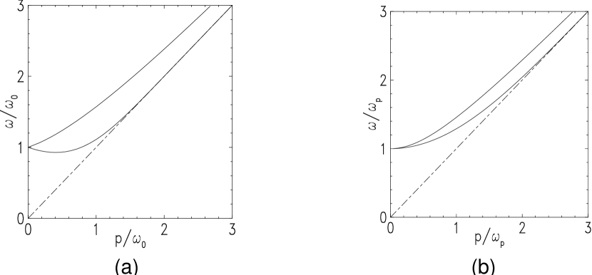
Figure 6: Dispersion relation for soft excitations in the linear regime: (a) soft fermions; (b) soft gluons (or linear plasma waves), with the upper (lower) branch corresponding to transverse (longitudinal) polarization.

The dispersion relations for the modes are obtained from the poles of the propagators, that is,

$${p}^{2}+\Pi_{L}(\omega_{L},p)=0,\qquad\omega_{T}^{2}=p^{2}+\Pi_{T}(\omega_{T},p),$$ (106)

for longitudinal and transverse excitations, respectively. The solutions to these equations, $\omega_{L}(p)$ and $\omega_{T}(p)$, are displayed in Fig. 6.b. The longitudinal mode is the analog of the familiar plasma oscillation. It corresponds to a collective oscillation of the hard particles, and disappears when $p\gg gT$. Both dispersion relations are time-like ($\omega_{L,T}(p)>p$), and show a gap at zero momentum (the same for transverse and longitudinal modes since, when $p\to 0$, we recover isotropy). With increasing momentum, the transverse branch becomes that of a relativistic particle with an effective mass $m_{\infty}\equiv m_{D}/\sqrt{2}$ (commonly referred to as the “asymptotic mass”). Although, strictly speaking, the HTL approximation does not apply at hard momenta, the above dispersion relation $\omega_{T}(p)$ remains nevertheless correct for $p\sim T$ where it coincides with the light-cone limit of the full one-loop result Kraemmer94 :

$$m_{\infty}^{2}\,\equiv\,\Pi_{T}^{1-loop}(\omega^{2}=p^{2})\,=\,{m_{D}^{2}\over 2}.$$ (107)

The dispersion relations of soft fermionic excitations exhibit also collective feature with a characteristic splitting at low momenta (see Fig. 6.a). We shall not discuss here this interesting phenomenon (see BIO95 and references therein).

We note finally that particular solutions of the non-linear equations (101) have also been found, in prl2 ; planew ; BIO95 . These solutions describe non-linear plane-waves propagating through the plasma, and represent truly non-Abelian collective excitations.

6.2 Debye screening

The screening of a static chromoelectric field by the plasma constituents is the natural non-Abelian generalization of the Debye screening, a familiar phenomenon in classical plasma physics PhysKin . In coordinate space, screening reduces the range of the gauge interactions. In momentum space, it contributes to regulate the infrared behaviour of the various $n$-point functions.

Screening properties can be inferred from an analysis of the effective photon (or gluon) propagators (104) in the static limit $\omega\to 0$. We have:

$$\Pi_{L}(0,p)\,=\,m_{D}^{2}\,,\qquad\,\,\,\,\Pi_{T}(0,p)=0,$$ (108)

and therefore:

$${}^{*}\!\Delta_{L}(0,p)\,=\,{-1\over p^{2}+m_{D}^{2}}\,,\qquad{}^{*}\!\Delta_{T}(0,p)\,=\,{1\over p^{2}}\,,$$ (109)

which clearly shows that the Debye mass $m_{D}$ acts as an infrared cut-off $\sim gT$ in the electric sector, while there is no such cut-off in the magnetic sector.

6.3 Landau damping

For time-dependent fields, there exists a different screening mechanism associated to the energy transfer to the plasma constituents. In Abelian plasmas, this mechanism is known as Landau damping PhysKin . The mechanical work done by a longwavelength electromagnetic field acting on the charged particles leads to an energy transfer PhysKin :

$${{\rm d}\,{\rm E}_{W}(t)\over{\rm d}\,t}\,=\,\int{\rm d}^{3}{\bf x}\,{\bf E}(t,\,{\bf x})\cdot{\bf j}(t,\,{\bf x}),$$ (110)

where $j^{i}(p)=\Pi_{R}^{i\nu}(p)A_{\nu}(p)$ is the induced current. One can then show that the average energy loss is related to the imaginary part of the retarded polarization tensor. From (75) we get:

$${\rm Im}\,\Pi_{R}^{\mu\nu}(\omega,{\bf p})\,=\,-\,\pi m_{D}^{2}\,\omega\int{{\rm d}\Omega\over 4\pi}\,\,v^{\mu}v^{\nu}\,\delta(\omega-{\bf v}\cdot{\bf p})\,.$$ (111)

The $\delta$-function in (111) shows that the particles which absorb energy are those moving in phase with the field (i.e., the particles whose velocity component along ${\bf p}$ is equal to the field phase velocity: ${\bf v}\cdot\hat{\bf p}=\omega/p$). Since in ultrarelativistic plasmas ${\bf v}$ is a unit vector, only space-like ($|\omega|<p$) fields are damped in this way.

To see how this mechanism leads to screening, consider the effective photon (or gluon) propagator (104), and focus on the magnetic propagator. For small but non-vanishing frequencies the corresponding polarization function $\Pi_{T}(\omega,p)$ is dominated by its imaginary part:

$$\Pi_{T}(\omega\ll p)\,=\,-i\,{\pi\over 4}\,m_{D}^{2}\,{\omega\over p}+\,{\rm O}(\omega^{2}/p^{2})\,,$$ (112)

and therefore

$${}^{*}\!\Delta_{T}(\omega\ll p)\simeq\,{1\over p^{2}-i\,(\pi\omega/4p)\,m_{D}^{2}}.$$ (113)

Thus Im$\,\Pi_{T}(p)$ acts as a frequency-dependent IR cutoff at momenta $p\sim(\omega m_{D}^{2})^{1/3}$. That is, as long as the frequency $\omega$ is different from zero, the soft momenta are dynamically screened by Landau damping Baym90 .

7 The entropy of the quark-gluon plasma

We come now to the last part of these lectures which will be mainly devoted to an introduction to the recent progress made in the calculation of the entropy of the quark-gluon plasma. We first comment on various aspects of perturbation theory and show that it is not appropriate for calculating the thermodynamics of the quark-gluon plasma, even a high temperature where the coupling is weak. The main source of difficulties is that the contributions of the collective modes, for which we have constructed an effective theory in the previous sections, are non perturbative and cannot be expanded in powers of the coupling constant. We then show that these contributions can be included by using self-consistent approximations familiar in many-body physics. These are best formulated for the entropy of the plasma, for which we obtain a simple approximation which provides an accurate description of lattice gauge calculations.

7.1 Results from perturbation theory

The free energy has been calculated up to order $g^{5}$, including the contribution of fermions Arnold94 . However, since our purpose here is mostly pedagogical, we shall limit our discussion to the gluon contribution at order $g^{4}$, in an SU(N) gauge theory. The pressure $P=-F/V$ can then be written:

$$P=P_{0}\left[1+a_{2}g^{2}+a_{3}g^{3}+\left(a_{4}(\mu/T)+a^{\prime}_{4}\ln g\right)g^{4}+O(g^{5})\right],$$ (114)

with

$$a_{2}=-5\left({\sqrt{N}\over 4\pi}\right)^{2},\,a_{3}={80\over\sqrt{3}}\left({\sqrt{N}\over 4\pi}\right)^{3},\,a_{4}^{\prime}=240\left({\sqrt{N}\over 4\pi}\right)^{4}\ln{\sqrt{N}\over 2\pi\sqrt{3}}$$ (116)

$$a_{4}=-5\left({\sqrt{N}\over 4\pi}\right)^{4}\left[{22\over 3}\ln{{\mu}\over 4\pi T}+{38\over 3}{\zeta^{\prime}(-3)\over\zeta(-3)}-{148\over 3}{\zeta^{\prime}(-1)\over\zeta(-1)}-4\gamma_{E}+{64\over 5}\right],$$

where $\zeta$ is Riemann’s zeta function, and $\mu$ the renormalization scale.

The first term in the expansion is $P_{0}$, the pressure of an ideal gas of gluons:

$$P_{0}=(N^{2}-1)\;T^{4}{\pi^{2}\over 45}.$$ (118)

The next term, of order $g^{2}$, is a genuine perturbative correction, and so is the term of order $g^{4}$. The contributions of order $g^{3}$ can be interpreted as a contribution of the collective modes to the pressure, and the odd power reflects the fact that the calculation of this contribution requires resummations. Similar resummations are responsible for the term in $g^{4}\ln g$.

We note that some of the coefficients in (116) depend on the renormalization scale $\mu$. However, the pressure itself should not depend on $\mu.$ It obeys a renormalization group equation:

$$\left[\mu^{2}{\partial\over\partial\mu^{2}}+\left(\mu^{2}{{\rm d}\alpha\over{\rm d}\mu^{2}}\right){\partial\over\partial\alpha}\right]P=0.$$ (119)

In this equation, $\alpha(\mu)\equiv g^{2}(\mu)/4\pi$ is the running coupling constant which satisfies the equation:

$$\mu^{2}{{\rm d}\alpha\over{\rm d}\mu^{2}}=\beta(\alpha)=-\beta_{2}\alpha^{2}-\beta_{3}\alpha^{3},$$ (120)

with

$$\beta_{2}={11N\over 12\pi},\qquad\qquad\beta_{3}={17N^{2}\over 24\pi^{2}}.$$ (121)

One can then show that, indeed, $P$ is independent of ${\mu}$: the explicit $\mu$ dependence of the coefficients cancels with that of the running coupling. Look indeed at the following combination of terms coming from the contributions of $a_{2}g^{2}$ and the $\mu$ dependent part of $a_{4}g^{4}$:

$${N\over 4\pi}\left\{\alpha+{N\over 4\pi}\alpha^{2}{22\over 3}\ln{{\mu}\over 4\pi T}\right\}.$$ (122)

By taking the derivative of this expression with respect to $\mu^{2}$ one gets:

$$\mu^{2}{\rm d\over{\rm d}\mu^{2}}\left\{{}\right\}=\mu^{2}{{\rm d}\alpha\over{\rm d}\mu^{2}}+{N\over 4\pi}\alpha^{2}{11\over 3}+{\rm\ higher\;order\;terms.}$$ (123)

By using the leading order expression of the $\beta$-function given in (120), one then obtains, as announced:

$$-{11\over 12\pi}N\;\alpha^{2}+{N\over 4\pi}\alpha^{2}{11\over 3}=0.$$ (124)

Note however, that the pressure is only formally independent of $\mu$ at order $g^{4}$, in the sense that its derivative with respect to $\mu$ involves terms of order $g^{5}$ at least. But the approximate expression (114) for $P$ does depend on $\mu$. As in all perturbative calculations, one is then led to look for the best value of $\mu$, i.e. the one which minimizes the higher order corrections. In the present context, a “natural choice” is to fix $\mu=2\pi T$, where $2\pi T$ is the scale provided by the basic Matsubara frequency. This choice makes the running coupling decrease with increasing temperature, and leads in particular to the expectation that the quark-gluon plasma becomes perturbative at very large temperature.

By calculating explicitly the various coefficients in (116) for $N=3$, one can write (114) thus:

$$P=P_{0}\left[1-0.095g^{2}+0.12g^{3}+\right.$$ (126)

$$\left.\left(0.09\ln g-0.007-0.013\ln\left({\mu\over 2\pi T}\right)\right)g^{4}+O(g^{5})\right].$$

Then, if for example one fixes $\mu=2\pi T$ and chooses a large temperature such that $\alpha(2\pi T)=0.1$, one gets $g=1.12$, and

$$P=P_{0}\left[1-0.12+0.17+0.004\right],$$ (127)

which shows no sign of convergence, with the term of order $g^{3}$ larger than the term of order $g^{2}$. Furthermore, if one analyzes the dependence of $P$ on the renormalization scale, on finds large variations as $\mu$ runs within the interval $\pi T<\mu<4\pi T$.

Attempts have been made to extract information from the first terms of this series using Pade approximants Hatsuda:1997wf ; Chiku:1998kd or Borel summation techniques Parwani:2001rr ; Parwani:2001am . The resulting expression of the pressure becomes indeed a smooth function of the coupling, better behaved than the polynomial approximation (114). These techniques however, which are in some situations very powerful, provide little physical insight, and we shall not discuss them further here.

The behavior of perturbation theory does not improve as one takes into account the higher order terms that one can calculate (namely orders $g^{4}$ and $g^{5}$). Furthermore, at order $g^{6}$, as we have already mentioned, perturbation theory becomes inapplicable because of infrared divergences. It has been shown in Braaten:1995na ; Braaten:1996ju ; Braaten:1996jr how, in principle, an effective theory could be constructed to overcome this particular problem by marrying analytical techniques (to determine the coefficients of the effective theory) and numerical ones (to solve the non perturbative 3-dimensional effective theory). The resulting effective theory is a 3-dimensional theory of static fields, with Lagrangian:

$${\cal L}_{eff}={1\over 4}(F^{a}_{ij})^{2}+{1\over 2}(D_{i}A_{0}^{a})^{2}+{1\over 2}m_{D}^{2}(A_{0}^{a})^{2}+\lambda(A_{0}^{a})^{4}+\delta{\cal L},$$ (128)

with $D_{i}=\partial_{i}-ig\sqrt{T}A_{i}$. This strategy has been applied recently to the calculation of the free energy of the quark-gluon plasma a high temperature Kajantie:2001iz . The slow convergence of the pressure towards the ideal gas value, that is seen in lattice calculations above $T_{c}$, is well reproduced. It is worth-emphasizing that this technique of dimensional reduction puts a special weight on the static sector (it singles out the contributions of the zero Matsubara frequency). However, as we shall see, it may be advantageous to keep, even in the calculation of equilibrium thermodynamic properties, the full spectral information that one has about the plasma excitations.

There are indeed indications that lattice data are well accounted for by simple phenomenological models of weakly interacting quasiparticles Peshier ; LH . In the case of the scalar field, the dominant effect of the interactions is to give a mass to the excitations. An indeed a perturbative expansion in terms of screened propagators (that is keeping the screening mass $\sim gT$ as a parameter, not considered as a term of order $g$ entering the expansion) has been shown to be quite stable with good convergence properties Karsch97 . In the case of gauge theory, the effect of the interactions is more complicated than just generating a mass. But we know how to determine the dominant corrections to the self-energies. When the momenta are soft, these are given by the hard thermal loops discussed above. By adding these corrections to the tree level Lagrangian, and subtracting them from the interaction part, one generated the so-called hard thermal loop perturbation theory ABS . The resulting perturbative expansion is made complicated however by the non local nature of the hard thermal loop action, and by the necessity of introducing temperature dependent counter terms. At the expense of some extra formalism, some of these difficulties can be avoided. This is discussed now.

7.2 Skeleton expansion for thermodynamic potential and entropy

In this section we recall the formalism of propagator renormalization that allow systematic rearrangements of the perturbative expansion while avoiding double-counting. We shall see in particular how self-consistent approximations can be used to obtain a simple expression for the entropy which isolates the contribution of the elementary excitations as a leading contribution. For pedagogical purposes, we shall mainly consider in these lectures the example of the scalar field.

The thermodynamic potential $\Omega=-PV$ of the scalar field can be written as the following functional of the full propagator $D$ LW ; Baym :

$$\beta\Omega[D]=-\log Z={1\over 2}{\,\mathrm{T}r\,}\log D^{-1}-{1\over 2}{\,\mathrm{T}r\,}\Pi D+\Phi[D]\,,$$ (129)

where ${\,\mathrm{T}r\,}$ denotes the trace in configuration space, $\beta=1/T$, $\Pi$ is the self-energy related to $D$ by Dyson’s equation ($D_{0}$ denotes the bare propagator):

$$D^{-1}=D^{-1}_{0}+\Pi,$$ (130)

and $\Phi[D]$ is the sum of the 2-particle-irreducible “skeleton” diagrams

$$-\Phi[D]=\includegraphics[bb=50 390 550 430,width=199.16928pt]{phi.ps}$$ (131)

The essential property of the functional $\Omega[D]$ is to be stationary under variations of $D$ (at fixed $D_{0}$) around the physical propagator. The physical pressure is then obtained as the value of $\Omega[D]$ at its extremum. The stationarity condition,

$${\delta\Omega[D]/\delta D}=0,$$ (132)

implies the following relation

$$\delta\Phi[D]/\delta D={1\over 2}\Pi,$$ (133)

which, together with (130), defines the physical propagator and self-energy in a self-consistent way. The equation (133) expresses the fact that the skeleton diagrams contributing to $\Pi$ are obtained by opening up one line of a two-particle-irreducible skeleton. Note that while the diagrams of the bare perturbation theory, i.e., those involving bare propagators, are counted once and only once in the expression of $\Pi$ given above, the diagrams of bare perturbation theory contributing to the thermodynamic potential are counted several times in $\Phi$. The extra terms in (129) precisely correct for this double-counting.

Self-consistent (or variational) approximations, i.e., approximations which preserve the stationarity property (132), are obtained by selecting a class of skeletons in $\Phi[D]$ and calculating $\Pi$ from (133). Such approximations are commonly called “$\Phi$-derivable” Baym .

The traces over configuration space in (129) involve integration over imaginary time and over spatial coordinates. Alternatively, these can be turned into summations over Matsubara frequencies and integrations over spatial momenta:

$$\int_{0}^{\beta}{\rm d}\tau\int{\rm d}^{3}x\rightarrow\beta V\int[{\rm d}k],$$ (134)

where $V$ is the spatial volume, $k^{\mu}=(i\omega_{n},{\bf k})$ and $\omega_{n}=n\pi T$, with $n$ even (odd) for bosonic (fermionic) fields (the fermions will be discussed later). We have introduced a condensed notation for the the measure of the loop integrals (i.e., the sum over the Matsubara frequencies $\omega_{n}$ and the integral over the spatial momentum ${\bf k}$):

$$\int[{\rm d}k]\equiv T\sum_{n,even}\int{{\rm d}^{3}k\over(2\pi)^{3}}$$ (135)

Strictly speaking, the sum-integrals in equations like (129) contain ultraviolet divergences, which requires regularization (e.g., by dimensional continuation). Since, however, most of the forthcoming calculations will be free of ultraviolet problems, we do not need to specify here the UV regulator (see however Sect. 7.3 for explicit calculations).

For the purpose of developing approximations for the entropy it is convenient to perform the summations over the Matsubara frequencies. One obtains then integrals over real frequencies involving discontinuities of propagators or self-energies which have a direct physical significance. Using standard contour integration techniques, one gets:

$$\Omega/V=\int\!\!{d^{4}k\over(2\pi)^{4}}\,n(\omega)\left(\rm Im\log(-\omega^{2}+k^{2}+\Pi)-\rm Im\Pi D\right)+T\Phi[D]/V$$ (136)

where $n(\omega)=1/({\rm e}^{\beta\omega}-1)$.

The analytic propagator $D(\omega,k)$ can be expressed in terms of the spectral function:

$$D(\omega,k)=\int_{-\infty}^{\infty}{dk_{0}\over 2\pi}{\rho(k_{0},k)\over k_{0}-\omega}.$$ (138)

and we define, for $\omega$ real,

$$\rm ImD(\omega,k)\equiv\rm ImD(\omega+i\epsilon,k)={\rho(\omega,k)\over 2}.$$ (139)

The imaginary parts of other quantities are defined similarly.

We are now in the position to calculate the entropy density:

$${\cal S}=-{\partial(\Omega/V)/\partial T}\,.$$ (140)

The thermodynamic potential, as given by (136) depends on the temperature through the statistical factors $n(\omega)$ and the spectral function $\rho$, which is determined entirely by the self-energy. Because of (132) the temperature derivative of the spectral density in the dressed propagator cancels out in the entropy density and one obtains Riedel ; VB :

$${\cal S} = -\int\!\!{d^{4}k\over(2\pi)^{4}}{\partial n(\omega)\over\partial T}\rm Im\log D^{-1}(\omega,k)$$ (142)

$$+\int\!\!{d^{4}k\over(2\pi)^{4}}{\partial n(\omega)\over\partial T}\rm Im\Pi(\omega,k)\rm ReD(\omega,k)+{\cal S}^{\prime}$$

with

$${\cal S}^{\prime}\equiv-{\partial(T\Phi)\over\partial T}\Big{|}_{D}+\int\!\!{d^{4}k\over(2\pi)^{4}}{\partial n(\omega)\over\partial T}\rm Re\Pi\,\rm ImD.$$ (143)

For the two-loop skeletons, we have:

$${\cal S}^{\prime}=0.$$ (144)

Loosely speaking, the first two terms in (142) represent essentially the entropy of “independent quasiparticles”, while ${\cal S}^{\prime}$ accounts for a residual interaction among these quasiparticles VB .

The vanishing of ${\cal S}^{\prime}$ holds whether the propagator are the self-consistent propagators or not. That is, only the relation (133) is used in the proof which does not require $D$ to satisfy the self-consistent Dyson equation (130). A general analysis of the contributions to ${\cal S}^{\prime}$ and their physical interpretation can be found in CP2 .

We emphasize now a few attractive features of the formula (142) with ${\cal S}^{\prime}=0$, which makes the entropy a privileged quantity to study the thermodynamics of ultrarelativistic plasmas. We note first that the formula for $\cal S$ at 2-loop order involves the self-energy only at 1-loop order. Besides this important simplification, this formula for ${\cal S}$, in contrast to the pressure, has the advantage of manifest ultra-violet finiteness, since ${\partial n/\partial T}$ vanishes exponentially for both $\omega\to\pm\infty$. Also, any multiplicative renormalization $D\to ZD$, $\Pi\to Z^{-1}\Pi$ with real $Z$ drops out from (142). Finally, the entropy has a more direct quasiparticle interpretation than the pressure. This will be illustrated explicitly in the simple model of the next subsection.

7.3 A simple model

In this section we shall present the self-consistent solution for the $(\lambda/4!)\phi^{4}$ theory, keeping in $\Phi$ only the two-loop skeleton. Anticipating the fact that the fully dressed propagator will be that of a massive particle, we write the spectral function as $\rho(k_{0},{\bf k})=2\pi\,\epsilon(k_{0})\,\delta(k_{0}^{2}-{\bf k}^{2}-m^{2})$, and consider $m$ as a variational parameter. The thermodynamic potential (129), or equivalently the pressure, becomes then a simple function of $m$. By Dyson’s equation, the self-energy is simply $\Pi=m^{2}$. We set:

$$I(m)\,\equiv\,{1\over 2}\int[{\rm d}k]\,D(k)\,={1\over 2}\int[{\rm d}k]\,{1\over\omega_{n}^{2}+{\bf k}^{2}+m^{2}}.$$ (145)

Then the pressure $P=-\Omega/V$ can be written as:

$$-P={1\over 2}\int{{\rm d}^{3}k\over(2\pi)^{3}}\varepsilon_{k}+{1\over\beta}\int{{\rm d}^{3}k\over(2\pi)^{3}}\log(1-{\rm e}^{-\beta\varepsilon_{k}})-m^{2}I(m)+{\lambda_{0}\over 2}I^{2}(m),$$ (146)

where $\varepsilon_{k}^{2}\equiv k^{2}+m^{2}$. By demanding that $P$ be stationary with respect to $m$ one obtains the self-consistency condition which takes here the form of a “gap equation”:

$$m^{2}\,=\,{\lambda_{0}}\,I(m).$$ (148)

The pressure in the two-loop $\Phi$-derivable approximation, as given by (145)–(148), is formally the same as the pressure per scalar degree of freedom in the (massless) $N$-component model with the interaction term written as ${3\over N+2}(\lambda/4!)(\phi_{i}\phi_{i})^{2}$ in the limit $N\to\infty$ Drummond:1998cw . From the experience with this latter model, we know that (145)–(148) admit an exact, renormalizable solution which we recall now.

At this stage, we need to specify some properties of the loop integral $I(m)$ which we can write as the sum of a vacuum piece $I_{0}(m)$ and a finite temperature piece $I_{T}(m)$ such that, at fixed $m$, $I_{T}(m)\to 0$ as $T\to 0$. We use dimensional regularization to control the ultraviolet divergences present in $I_{0}$, which implies $I_{0}(0)=0$. Explicitly one has:

$$\mu^{\epsilon}I(m)=-{m^{2}\over 32\pi^{2}}\left({2\over\epsilon}+\log{\bar{\mu}^{2}\over m^{2}}+1\right)+I_{T}(m)+{\rm O}(\epsilon),$$ (149)

with

$$I_{T}(m)=\int\!\!{d^{3}k\over(2\pi)^{3}}\,{n(\varepsilon_{k})\over 2\varepsilon_{k}}\,,$$ (150)

and $\varepsilon_{k}\equiv(k^{2}+m^{2})^{1/2}$. In (149), $\mu$ is the scale of dimensional regularization, introduced, as usual, by rewriting the bare coupling $\lambda_{0}$ as $\mu^{\epsilon}\hat{\lambda}_{0}$, with dimensionless $\hat{\lambda}_{0}$; furthermore, $\epsilon=4-n$, with $n$ the number of space-time dimensions, and $\bar{\mu}^{2}=4\pi{\rm e}^{-\gamma}\mu^{2}$.

We use the modified minimal subtraction scheme ($\overline{\hbox{MS}}$) and define a dimensionless renormalized coupling $\lambda$ by:

$${1\over\lambda}={1\over\lambda_{0}\mu^{-\epsilon}}+{1\over 16\pi^{2}\epsilon}.$$ (151)

When expressed in terms of the renormalized coupling, the gap equation becomes free of ultraviolet divergences. It reads:

$$m^{2}\,=\,{\lambda\over 2}\int{{\rm d}^{3}k\over(2\pi)^{3}}\,{n(\varepsilon_{k})\over\varepsilon_{k}}\,+\,{\lambda m^{2}\over 32\pi^{2}}\left(\log{m^{2}\over\bar{\mu}^{2}}\,-1\right),$$ (152)

The renormalized coupling constant satisfies

$${{\rm d}\lambda\over{\rm d}\log\bar{\mu}}\,=\,{\lambda^{2}\over 16\pi^{2}},$$ (153)

which ensures that the solution $m^{2}$ of (152) is independent of $\bar{\mu}$. The expression (153) coincides with the exact $\beta$-function in the large-$N$ limit, but gives only one third of the lowest-order perturbative $\beta$-function for $N=1$. This is no actual fault since the running of the coupling affects the thermodynamic potential only at order $\lambda^{2}$ which is beyond the perturbative accuracy of the 2-loop $\Phi$-derivable approximation. In order to see the correct one-loop $\beta$-function at finite $N$, the approximation for $\Phi$ would have to be pushed to 3-loop order.

Note also that, in the present approximation, the renormalization (151) of the coupling constant is sufficient to make the pressure (146) finite. Indeed, in dimensional regularization the sum of the zero point energies ${\varepsilon_{k}}/2$ in (146) reads:

$$\mu^{\epsilon}\int{{\rm d}^{n-1}k\over(2\pi)^{n-1}}\,\,{\varepsilon_{k}\over 2}\,=\,-{m^{4}\over 64\pi^{2}}\left({2\over\epsilon}+\log{\bar{\mu}^{2}\over m^{2}}+{3\over 2}\right)+{\rm O}(\epsilon),$$ (154)

so that

$$\mu^{\epsilon}\int{{\rm d}^{n-1}k\over(2\pi)^{n-1}}\,\,{\varepsilon_{k}\over 2}\,-\,{\Pi^{2}\over 2\hat{\lambda}_{0}}\,=\,-\,{m^{4}\over 2\lambda}\,-\,{m^{4}\over 64\pi^{2}}\left(\log{\bar{\mu}^{2}\over m^{2}}+{3\over 2}\right)+{\rm O}(\epsilon)$$ (155)

is indeed UV finite as $n\to 4$. After also using the gap equation (152), one obtains the $\bar{\mu}$-independent result

$$P=-T\int{{\rm d}^{3}k\over(2\pi)^{3}}\,\log(1-{\rm e}^{-\beta\varepsilon_{k}})+{m^{2}\over 2}I_{T}(m)+{m^{4}\over 128\pi^{2}}.$$ (156)

We now compute the entropy according to (142). Since $\rm Im\Pi=0$ and $\rm Re\Pi=m^{2}$, we have simply:

$${\cal S}=-\int\!\!{d^{4}k\over(2\pi)^{4}}{\partial n(\omega)\over\partial T}\rm Im\log(k^{2}-\omega^{2}+m^{2}).$$ (157)

Using

$$\rm Im\log(k^{2}-\omega^{2}+m^{2})\,=\,-\pi\epsilon(\omega)\theta(\omega^{2}-\varepsilon_{k}^{2}),$$ (158)

and the identity,

$${\partial n(\omega)\over\partial T}=-\,{\partial\sigma(\omega)\over\partial\omega},\qquad\sigma(\omega)\equiv-n\log n+(1+n)\log(1+n),$$ (159)

one can rewrite (157) in the form (with $n_{k}\equiv n(\varepsilon_{k})$):

$${\cal S}=\int\!\!{d^{3}k\over(2\pi)^{3}}\Bigl{\{}(1+n_{k})\log(1+n_{k})\,-\,n_{k}\log n_{k}\Bigr{\}}.$$ (160)

This formula shows that, in the present approximation, the entropy of the interacting scalar gas is formally identical to the entropy of an ideal gas of massive bosons, with mass $m$.

It is instructive to observe that such a simple interpretation does not hold for the pressure. The pressure of an ideal gas of massive bosons is given by:

$$P^{(0)}(m) = \int\!\!{d^{3}k\over(2\pi)^{3}}\int_{\epsilon_{k}}^{\infty}{\rm d}\omega\left(n(\omega)+{1\over 2}\right)$$ (161)

$$= -\int\!\!{d^{3}k\over(2\pi)^{3}}\left\{T\log(1-{\rm e}^{-\epsilon_{k}/T})+{\epsilon_{k}\over 2}\right\},$$ (162)

which differs indeed from (146) by the term $m^{4}/\lambda$ which corrects for the double-counting of the interactions included in the thermal mass.

7.4 Comparison with thermal perturbation theory

In view of the subsequent application to QCD, where a fully self-consistent determination of the gluonic self-energy seems prohibitively difficult, we shall be led to consider approximations to the gap equation. These will be constructed such that they reproduce (but eventually transcend) the perturbative results up to and including order $\lambda^{3/2}$ or $g^{3}$, which is the maximum perturbative accuracy allowed by the approximation ${\cal S}^{\prime}=0$.

In view of this it is important to understand the perturbative content of the self-consistent approximations for $m^{2}$, $P$ and ${\cal S}$. In this section we shall demonstrate that, when expanded in powers of the coupling constant, these approximations reproduce the correct perturbative results up to order $\lambda^{3/2}$ Kapusta . This will also elucidate how perturbation theory gets reorganized by the use of the skeleton representation together with the stationarity principle.

For the scalar theory with only $(\lambda/4!)\,\phi^{4}$ self-interactions, we write $\lambda\equiv 24g^{2}$, and compute the corresponding self-energy $\Pi=m^{2}$ by solving the gap equation (152) in an expansion in powers of $g$, up to order $g^{3}$. Since we anticipate $m$ to be of order $gT$, we can ignore the second term $\propto\lambda m^{2}\sim g^{4}$ in the r.h.s. of (152), and perform a high-temperature expansion of the integral $I_{T}(m)$ in the first term (cf. (150)) up to terms linear in $m$. This gives the following, approximate, gap equation:

$$m^{2}\,\simeq\,g^{2}T^{2}-{3\over\pi}\,g^{2}Tm\,.$$ (163)

The first term in the r.h.s. arises as

$$24g^{2}I_{T}(0)\,=\,12g^{2}\int\!\!{d^{3}k\over(2\pi)^{3}}\,{n(k)\over k}\,=\,g^{2}T^{2}\,\equiv\,\hat{m}^{2}.$$ (164)

This is also the leading-order result for $m^{2}$, commonly dubbed the “hard thermal loop”.

The second term, linear in $m$, in (163) comes from

$$12g^{2}\int\!\!{d^{3}k\over(2\pi)^{3}}\left({n(\varepsilon_{k})\over\varepsilon_{k}}-{n(k)\over k}\right)\,\simeq\,$$ (165)

(166)

$$\qquad\qquad 12g^{2}T\int\!\!{d^{3}k\over(2\pi)^{3}}\left({1\over k^{2}+m^{2}}-{1\over k^{2}}\right)\,=\,-{3g^{2}\over\pi}mT\,,$$ (167)

where we have used the fact that the momentum integral is saturated by soft momenta $k\sim gT$, so that to the order of interest $n(\varepsilon_{k})\simeq T/\varepsilon_{k}$ (and similarly $n(k)\simeq T/k$). This provides the next-to-leading order (NLO) correction to the thermal mass

$$\delta m^{2}\,\equiv\,-{3g^{2}\over\pi}\hat{m}T\,=\,-{3\over\pi}\,g^{3}T^{2}\,.$$ (168)

Thus, to order $g^{3}$, one has $m^{2}=\hat{m}^{2}+\delta m^{2}$. In standard perturbation theoryKapusta ; LeBellac96 , the first term arises as the one-loop tadpole diagram evaluated with a bare massless propagator, while the second term comes from the same diagram where the internal line is soft and dressed by the HTL, that is $\hat{D}(\omega,k)\equiv-1/(\omega^{2}-k^{2}-\hat{m}^{2})$.

Consider similarly the perturbative estimates for the pressure and entropy, as obtained by evaluating (146) and (160) with the perturbative self-energy $\Pi=m^{2}\simeq\hat{m}^{2}+\delta m^{2}$, and further expanding in powers of $g$, to order $g^{3}$. The renormalized version of (146) yields, to this order (recall that $m\sim gT$ and $\lambda\sim g^{2}$),

$$P\,\simeq\,{\pi^{2}T^{4}\over 90}-{m^{2}T^{2}\over 24}+{m^{3}T\over 12\pi}+\cdots+{m^{4}\over 2\lambda}.$$ (169)

The first terms before the dots represent the pressure of massive bosons, i.e. (161) expanded up to third order in powers of $m/T$. From (169), it can be easily verified that the above perturbative solution for $m^{2}$ ensures the stationarity of $P$ up to order $g^{3}$, as it should. Indeed, if we denote

$$P_{2}(m)\,\equiv\,-{m^{2}T^{2}\over 24}\,+\,{m^{4}\over 2\lambda}\,,\qquad\,P_{3}(m)\,\equiv\,{m^{3}T\over 12\pi}\,,$$ (170)

then the following identities hold:

$${\partial P_{2}\over\partial m}\bigg{|}_{\hat{m}}\,=\,0,\qquad{\partial P_{2}\over\partial m}\bigg{|}_{\hat{m}+\delta m}\,+\,{\partial P_{3}\over\partial m}\bigg{|}_{\hat{m}}\,=\,0.$$ (171)

This shows that the NLO mass correction $\delta m^{2}\sim g^{3}T^{2}$ can be also obtained as

$$\delta m^{2}\,=\,-\,{(\partial P_{3}/\partial m)\over(\partial^{2}P_{2}/\partial m^{2})}\bigg{|}_{\hat{m}}\,=\,-{3g\over\pi}\,\hat{m}^{2}\,,$$ (172)

in agreement with (168). Moreover, $P_{2}\equiv P_{2}(\hat{m})=-g^{2}T^{2}/48$ and $P_{3}\equiv P_{3}(\hat{m})=\hat{m}^{3}T/12\pi$ are indeed the correct perturbative corrections to the pressure, to orders $g^{2}$ and $g^{3}$, respectively Kapusta . In fact, the pressure to this order can be written as:

$$P = {\pi^{2}T^{4}\over 90}-{\hat{m}^{2}T^{2}\over 24}\,(1-{3\over\pi}\,g)+{\hat{m}^{3}T\over 12\pi}+\cdots\,+\,{\hat{m}^{4}\over 2\lambda}\,(1-{3\over\pi}\,g)^{2}+{\cal O}(g^{4})$$ (173)

$$= {\pi^{2}T^{4}\over 90}-{\hat{m}^{2}\over 48}T^{2}+{\hat{m}^{3}T\over 12\pi}\,.$$ (174)

Note that the term of order $g^{2}$ is only half of that one would obtain from (161) by replacing $m$ by $\hat{m}$. This is due to the mismatch between (161) and the correct expression (146) for the pressure. In fact the net order $g^{2}$ contribution to the pressure comes from $\Phi$ evaluated with bare propagators: the order $g^{2}$ contributions in the other two terms mutually cancel indeed. This is to be expected: there is a single diagram of order $g^{2}$; this is a skeleton diagram, counted therefore once and only once in $\Phi$. Observe also that the terms of order $g^{3}$ originating from the terms $\hat{m}^{2}$ and $\hat{m}^{4}$ mutually cancel; that is, the NLO mass correction $\delta m$ drops out from the pressure up to order $g^{3}$. This is no accident: the cancellation results from the stationarity of $P$ at order $g^{2}$, the first equation (171).

Consider now the entropy density. The correct perturbative result up to order $g^{3}$ may be obtained directly by taking the total derivative of the pressure, (173) with respect to $T$. One then obtains:

$${\cal S}={4\over T}\left({\pi^{2}T^{4}\over 90}-{\hat{m}^{2}T^{2}\over 48}+{\hat{m}^{3}T\over 12\pi}\right)+{\cal O}(g^{4}).$$ (175)

We wish, however, to proceed differently, using (160), or equivalently, since $\partial P/\partial m=0$ when $m$ is a solution of the gap equation, by writing:

$${\cal S}=\left.{\partial P\over\partial T}\right|_{m}.$$ (176)

This yields:

$${\cal S}={4\over T}\left({\pi^{2}T^{4}\over 90}-{m^{2}T^{2}\over 48}+{m^{3}T\over 48\pi}\right)+{\cal O}(m^{4}/T),$$ (177)

which coincides as expected with the expression obtained by expanding the entropy (160) of massive bosons, up to order $(m/T)^{3}$. If we now replace $m$ by its leading order value $\hat{m}$, the resulting approximation for ${\cal S}$ reproduces the perturbative effect of order $\sim g^{2}$, but it underestimates the correction of order $g^{3}$ by a factor of 4. This is corrected by changing $m$ to $\hat{m}+\delta m$ with $\delta m=-3g\hat{m}/2\pi$ in the second order term of (177). Note that although it makes no difference to enforce the gap equation to order $g^{3}$ in the pressure (because of the cancellation discussed above), there is no such cancellation in the entropy.

7.5 Approximately self-consistent solutions

As we have seen, the 2-loop $\Phi$-derivable approximation provides an expression for the entropy ${\cal S}$ as a functional of the self-energy $\Pi$ which has a simple quasiparticle interpretation and is manifestly ultraviolet finite for any (finite) $\Pi$. These attractive features of the formula (142) are independent of the specific form of the self-energy, and will be shown to hold in QCD as well. Of course, within this approximation, the self-energy is uniquely specified: by the stationarity principle, this is given by the self-consistent solution to the one-loop gap equation. In the scalar $\phi^{4}$-model, it was easy to give the exact solution to this equation. In QCD, however, it will turn out that a fully self-consistent solution is both prohibitively difficult (because of the non-locality of the gap equation), and not really desirable (because gauge symmetry implies relations between the renormalization of the propagators and that of the vertices, and the present approximation deals only with propagator renormalization). This leads us to consider approximately self-consistent resummations, which are obtained in two steps: (a) An approximation is constructed for the solution $\Pi$ to the gap equation, and (b) the entropy (142) is evaluated exactly (i.e., numerically) with this approximate self-energy. While step (b) above is unambiguous and inherently non-perturbative, step (a), on the other hand, will be constrained primarily by the requirement of preserving the maximum possible perturbative accuracy, of order $g^{3}$. In addition to that, we shall add the qualitative requirement that the approximation for $\Pi$, and the ensuing one for ${\cal S}$, are well defined and physically meaningful for all the values of $g$ of interest, and not only for small $g$—that is, for all the values of $g$ where the fully self-consistent calculation makes sense a priori. Finally, in the case of QCD, relaxing the requirement of complete self-consistency allows us to construct gauge invariant approximations.

Figure 7: QCD skeletons contributing to $\Phi$ at 2-loop order. Wiggly, plain and dotted lines refer respectively to gluons, quarks and ghosts

We shall now, in the rest of this lecture, outline the main steps that are involved in the implementation of these approximations in the case of QCD. Details can be found in the original publications Blaizot:1999ip ; Blaizot:1999ap ; Blaizot:2001fc .

At 2-loop order, the relevant skeletons are displayed in Fig. 7. By itself, the corresponding self-consistent truncation is not a gauge invariant approximation. Our strategy then will be to use gauge-invariant approximations to self-energies, in place of the self-consistent ones. These self-energies are then used to compute the entropy without further approximations. In complete analogy with the example of the scalar case that we have discussed in the previous section, these approximations are such that, when expanded in powers of the coupling the entropy is identical to that given by perturbation theory up to and including order $g^{3}$.

Figure 8: Next to leading order contribution to $\delta\Pi_{T}$ (top) and to $\delta\Sigma$ (bottom) at hard momentum. Thick dashed and wiggly lines with a blob represent HTL-resummed longitudinal and transverse propagators, respectively

The approximate self-energies that we use are the hard thermal loops discussed above. Namely, for soft momenta $\omega,\,p\sim gT$, we take $\Pi_{soft}\,\approx\,\Pi_{HTL}$ and $\Sigma_{soft}\,\approx\,\Sigma_{HTL}$, for gluons and quarks respectively. We shall also need an approximation valid for $\omega,\,p\sim T$: $\Pi_{hard}(\omega^{2}\sim p^{2})$ and similarly for $\Sigma$. It turns out that this is accurately given by the hard thermal loop, even though the momenta are not soft Kraemmer94 . All these approximations are gauge invariant. The corresponding diagrams are displayed in Figs. 8.

We can then proceed exactly as in the scalar case. As a first approximation one may simply use the hard thermal loops $\Pi=\Pi_{HTL}$ and $\Sigma\sim\Sigma_{HTL}$ at all momenta; we refer to the corresponding entropy as ${\cal S}={\cal S}_{HTL}$. The perturbative content of this approximation is schematically ${\cal O}(g^{2})\,+\,,{1\over 4}\,{\cal O}(g^{3})$; that is, the approximation fully accounts or the order $g^{2}$, but reproduce only a quarter of the $g^{3}$ order, exactly as in the scalar case. In the next-to-leading approximation, we correct the hard degrees of freedom by their interaction with the soft modes. That is, we continue to use the hard thermal loops at small momenta, but use at hard momenta the corrections corresponding to the diagrams displayed in Fig. 8. The resulting approximation to the entropy, ${\cal S}={\cal S}_{NLA}$ accounts then fully for the orders $g^{2}$ and $g^{3}$. But of course these expressions are not limited to values of the coupling as small as required for the validity of perturbation theory.

7.6 Some results for QCD

As an illustration of the quality of the results that are obtained within that scheme, we show in Fig. 9 the entropy of pure SU(3) gauge theory. The bands delimiting the various lines in this figure correspond to varying the $\overline{\rm MS}$ renormalization scale $\bar{\mu}$, which defines the renormalized coupling constant $g(\bar{\mu})$, from $\bar{\mu}=\pi T$ to $4\pi T$. One sees that in contrast to ordinary perturbation theory, going from one level of approximation to the next one is indeed a small correction. In particular the effects of the soft modes is here a small contribution. This is o be contrasted with perturbation theory where the order $g^{3}$ contribution is large for moderate values of the coupling. The comparison with the lattice data Boyd is quite good down to $T\mathrel{\hbox to0.0pt{\raise 2.20013pt\hbox{$>$}\hss}{\lower 2.20013pt\hbox{$\sim$}}}2.5T_{c}$.

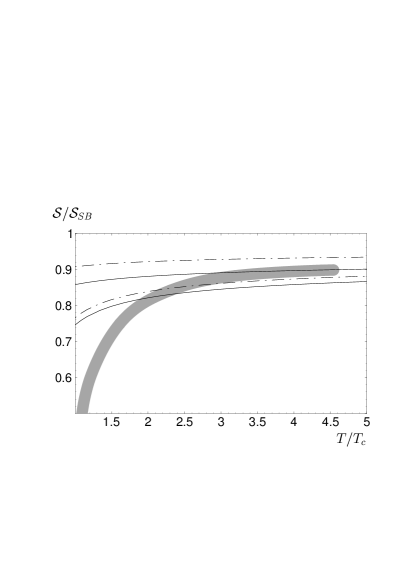
Figure 9: The entropy of pure SU(3) gauge theory normalized to the ideal gas entropy ${\cal S}_{0}$. Full lines: ${\cal S}_{HTL}$. Dashed-dotted lines: ${\cal S}_{NLA}$. 2-loop $\beta$-function $\rightarrow$ the running coupling constant $\alpha_{s}(\bar{\mu})$. The $\overline{{\rm MS}}$ renormalization scale: $\bar{\mu}=\pi T\cdots 4\pi T$. The dark grey band: lattice result by Boyd et al (1996)

The quality of the agreement between the self-consistent approximation and the lattice data supports the quasiparticle picture of the quark-gluon plasma: the dominant effect of the interactions at high temperature seems to be to change the bare quarks and gluons into massive quasiparticles, with small residual interactions between the quasiparticles. It should be emphasized that, in contrast to the approximations based on dimensional reduction, the method makes full use of the spectral information on the quasiparticles contained in particular in the hard thermal loops.

The approach is easily extended to finite chemical potential, and the calculation of the baryonic density can be done using approximations similar to those we used for the entropy. Furthermore, from the knowledge of $N(\mu,T)$ and $S(\mu,T)$ one can reconstruct $P(\mu,T)$. Use lattice data to fix the integration constant (e.g. $P(\mu=0,T)$). Such investigations are underway.

References

- (1)
- (2) J. Blaizot and E. Iancu, “The quark-gluon plasma: Collective dynamics and hard thermal loops,” to appear in Phys. Rept, hep-ph/0101103.
- (3) J.P. Blaizot, “QCD at finite temperature”, in “Probing the Standard Model of Particle Interactions”, Les Houches, Session LXVIII, 1997, ed. by R. Gupta et al. (Elsevier, Amsterdam, 1999).
- (4) J. P. Blaizot, “The quark-gluon plasma and nuclear collisions at high energy,” Lecture given at Les Houches Summer School on Theoretical Physics, Session 66: Trends in Nuclear Physics, 100 Years Later, Les Houches, France, 30 Jul - 30 Aug 1996.
- (5) J.-P. Blaizot, E. Iancu and J.-Y. Ollitrault, in Quark Gluon Plasma 2, R.C. Hwa ed., World Scientific, Singapore (1995), p. 135.
- (6) J.-P. Blaizot, in Lecture Notes on the Workshop: Nuclear Equation of State, Puri, India Jan. 1994, A. Ansari and L. Satpathy eds. (World Scientific, Singapore, 1996).
- (7) J-P. Blaizot, in Proceeding of Fourth Summer School and Symposium on Nuclear Physics, High Density and High Temperature Physics, July 1-6, Namwon, Korea, Journ. Korean Phys. Soc., vol. 25.
- (8) L. Kadanov and G. Baym, Quantum Statistical mechanics, (Benjamin/Cummings, London,1962).
- (9) A.A. Abrikosov, L.P. Gorkov and I.E. Dzyaloshinskii, Methods of Quantum Field Theory in Statistical Physics, (Dover, New-York, 1963).
- (10) A. Fetter and J.D. Walecka, Quantum Theory of Many Particle Systems, (McGraw Hill, New-York, 1971).
- (11) J.P. Blaizot and G. Ripka, Quantum Theory of Finite Systems, (MIT Press, Cambridge, 1986).
- (12) J.I. Kapusta, Finite temperature field theory, Cambridge Monographs in Mathematical Physics, (Cambridge University Press, 1989).
- (13) M. Le Bellac, Thermal field theory, Cambridge Monographs in Mathematical Physics, (Cambridge University Press, 1996).
- (14) J. P. Blaizot, E. Iancu and A. Rebhan, Phys. Rev. Lett. 83 (1999) 2906 [hep-ph/9906340].
- (15) J. P. Blaizot, E. Iancu and A. Rebhan, quark-gluon plasma,” Phys. Lett. B 470 (1999) 181 [hep-ph/9910309].
- (16) J. P. Blaizot, E. Iancu and A. Rebhan, of the quark-gluon plasma. I: Entropy and density,” Phys. Rev. D 63 (2001) 065003 [hep-ph/0005003].
- (17) K. Johnson, C.B. Thorn, A. Chodos, R.L. Jaffe and V.F. Weisskopf, Phys. Rev. D9 (1974) 3471; K. Johnson, A. Chodos, R.L. Jaffe and C.B. Thorn, Phys. Rev. D10 (1974) 2599.
- (18) P. Ginsparg, Nucl. Phys. B170 (1980) 388.
- (19) T. Appelquist and R.D. Pisarski, Phys. Rev. D23 (1981) 2305.
- (20) S. Nadkarni, Phys. Rev. D27 (1983) 917; Phys. Rev. D38 (1988) 3287.
- (21) N.P. Landsman, Nucl. Phys. B322 (1989) 498.
- (22) E. Braaten, Phys. Rev. Lett.74 (1995) 2164.
- (23) K. Kajantie, K. Rummukainen and M.E. Shaposhnikov, Nucl. Phys. B407 (1993) 356; K. Farakos, K. Kajantie, K. Rummukainen and M.E. Shaposhnikov, Nucl. Phys. B425 (1994) 67; ibidem 442 (1995) 317.
- (24) A.D. Linde, Rep. Progr. Phys. 42 (1979) 389.
- (25) A.D. Linde, Phys. Lett. B96 (1980) 289.
- (26) J.P. Blaizot and E. Iancu, Nucl. Phys. B390 (1993) 589.
- (27) J.P. Blaizot and E. Iancu, Phys. Rev. Lett.70 (1993) 3376; Nucl. Phys. B417 (1994) 608.
- (28) V.V. Klimov, Sov. J. Nucl. Phys.33 (1981) 934; Sov. Phys. JETP55 (1982) 199.
- (29) H.A. Weldon, Phys. Rev. D26 (1982) 1394.
- (30) H.A. Weldon, Phys. Rev. D26 (1982) 2789.
- (31) R. D. Pisarski, Phys. Rev. Lett.63 (1989) 1129; E. Braaten and R. D. Pisarski, Nucl. Phys. B337 (1990) 569; Nucl. Phys. B339 (1990) 310; Phys. Rev. Lett.64 (1990) 1338; Phys. Rev. D42 (1990) 2156.
- (32) J. Frenkel and J.C. Taylor, Nucl. Phys. B334 (1990) 199; J.C. Taylor and S.M.H. Wong, ibid. B346 (1990) 115.
- (33) R. Efraty and V.P. Nair, Phys. Rev. Lett.68 (1992) 2891; R. Jackiw and V.P. Nair, Phys. Rev. D48 (1993) 4991.
- (34) E.M. Lifshitz and L.P. Pitaevskii, Physical Kinetics (Pergamon Press, Oxford, 1981).
- (35) V.P. Silin, Sov. Phys. JETP11 (1960) 1136.
- (36) N.L. Balazs and B.K. Jennings, Phys. Repts.104 (1984) 347.
- (37) M. Hillery, R.F. O’Connell, M.O. Scully, and E.P. Wigner, Phys. Repts.106 (1984) 121.
- (38) G. Baym and C.J. Pethick, Landau Fermi-liquid theory: concepts and applications, (J. Wiley, N.Y., 1991).
- (39) S.K. Wong, Nuovo Cimento 65A (1970) 689.
- (40) U. Heinz, Phys. Rev. Lett.51 (1983) 351; J. Winter, J.Phys. (Paris) Suppl.45 (1984) C4-53; U. Heinz, Ann. Phys.161 (1985) 48.
- (41) H.-Th. Elze and U. Heinz, Phys. Repts.183 (1989) 81.
- (42) P.F. Kelly, Q. Liu, C. Lucchesi and C. Manuel, Phys. Rev. Lett.72 (1994) 3461; Phys. Rev. D50 (1994) 4209.
- (43) A. V. Selikhov and M. Gyulassy, Phys. Lett. B316 (1993) 373; Phys. Rev. C49 (1994) 1726.
- (44) Yu.A. Markov, M.A. Markova, Theor. Math. Phys. 103 (1995) 444.
- (45) U. Kraemmer, A. Rebhan and H. Schulz, Ann. Phys.238 (1995) 286.
- (46) J.P. Blaizot and E. Iancu, Phys. Rev. Lett.72 (1994) 3317.
- (47) J.P. Blaizot and E. Iancu, Phys. Lett. B326 (1994) 138.
- (48) G. Baym, H. Monien, C.J. Pethick, and D.G. Ravenhall, Phys. Rev. Lett.64 (1990) 1867.
- (49) P. Arnold and C. Zhai, Phys. Rev. D50 (1994) 7603; Phys. Rev. D51 (1995) 1906; C. Zhai and B. Kastening, Phys. Rev. D52 (1995) 7232. See also, E. Braaten, Phys. Rev. Lett.74 (1995) 2164; E. Braaten and A. Nieto, Phys. Rev. D51 (1995) 6990.
- (50) E. Braaten, Phys. Rev. Lett. 74 (1995) 2164 [hep-ph/9409434].
- (51) E. Braaten and A. Nieto, Phys. Rev. Lett. 76 (1996) 1417 [hep-ph/9508406].
- (52) E. Braaten and A. Nieto, Phys. Rev. D 53 (1996) 3421 [hep-ph/9510408].
- (53) K. Kajantie, M. Laine, K. Rummukainen and Y. Schroder, Phys. Rev. Lett. 86 (2001) 10 [hep-ph/0007109].
- (54) T. Hatsuda, Phys. Rev. D 56 (1997) 8111 [hep-ph/9708257].
- (55) S. Chiku and T. Hatsuda, Phys. Rev. D 58 (1998) 076001 [hep-ph/9803226].
- (56) R. R. Parwani, Yang-Mills theory,” Phys. Rev. D 63 (2001) 054014 [hep-ph/0010234].
- (57) R. R. Parwani, Phys. Rev. D 64 (2001) 025002 [hep-ph/0010294].
- (58) A. Peshier, B. Kämpfer, O. P. Pavlenko, and G. Soff, Phys. Rev. D 54, 2399 (1996); A. Peshier, hep-ph/9809379.
- (59) P. Lévai and U. Heinz, Phys. Rev. C 57, 1879 (1998) and references therein.
- (60) F. Karsch, A. Patkos and P. Petreczky, Phys. Lett. B401 (1997) 69.
- (61) J. O. Andersen, E. Braaten, and M. Strickland, Phys. Rev. Lett. 83, 2139 (1999), Phys. Rev. D 61, 014017, 074016 (2000).
- (62) J. M. Luttinger and J. C. Ward, Phys. Rev. 118, 1417 (1960); C. De Dominicis and P.C. Martin, J. Math. Phys. 5, 14, 31 (1964).
- (63) G. Baym, Phys. Rev. 127, 1391 (1962).
- (64) E. Riedel, Z. Phys. 210, 403 (1968).
- (65) B. Vanderheyden and G. Baym, J. Stat. Phys. 93, 843 (1998).
- (66) G. M. Carneiro and C. J. Pethick, Phys. Rev. B 11, 1106 (1975).
- (67) I. T. Drummond, R. R. Horgan, P. V. Landshoff and A. Rebhan, Nucl. Phys. B 524 (1998) 579 [hep-ph/9708426].
- (68) G. Boyd et al., Nucl. Phys. B469, 419 (1996).