July 2001

Electromagnetic corrections to $\gamma\pi^{\pm}\to\pi^{0}\pi^{\pm}$

Ll. Ametller^a, M. Knecht^b and P. Talavera^b

^a Dept. de Física i Enginyeria Nuclear, UPC
E-08034 Barcelona, Spain.
^b Centre de Physique Théorique, CNRS–Luminy, Case 907
F-13288 Marseille Cedex 9, France.

Abstract

The amplitude for the anomalous transitions $\gamma\pi^{\pm}\to\pi^{0}\pi^{\pm}$ is analyzed within Chiral Perturbation Theory including electromagnetic interactions. The presence of a $t$-channel one-photon exchange contribution induces sizeable ${\cal{O}}(e^{2})$ corrections which enhance the cross-section in the threshold region and bring the theoretical prediction into agreement with available data. In the case of the crossed reaction $\gamma\pi^{0}\rightarrow\pi^{+}\pi^{-}$, the same contribution appears in the s-channel and its effects are small.

PACS: 11.30.Rd, 12.39.Fe, 13.75.-n, 14.70.Bh, 13.60.Le

Keywords: Chiral Symmetry, Chiral Perturbation Theory, Scattering at low-energy, Meson production.

1 Introduction

The QCD matrix element of the electromagnetic current $j_{\mu}(x)$ between the vacuum and the three-pion state is described by a single invariant function $F^{3\pi}(s_{+},s_{-},s_{0})$, viz.

$$e\,\langle\Omega\,|j_{\mu}(0)|\,\pi^{+}(p_{+})\,\pi^{-}(p_{-})\,\pi^{0}(p_{0})\rangle\,=\,iF^{3\pi}(s_{+},s_{-},s_{0})\,\epsilon_{\mu\nu\alpha\beta}p_{0}^{\nu}p_{+}^{\alpha}p_{-}^{\beta}\,.\\$$ (1.1)

In the absence of isospin breaking, $F^{3\pi}(s_{+},s_{-},s_{0})$ is symmetric with respect to permutations of the three variables, with $s_{\pm}=(p_{\pm}+p_{0})^{2}$, $s_{0}=(p_{+}+p_{-})^{2}$, and $s_{+}+s_{-}+s_{0}=3M_{\pi}^{2}+q^{2}$, $q^{2}=(p_{+}+p_{-}+p_{0})^{2}$. Appropriate analytic continuations of $F^{3\pi}(s_{+},s_{-},s_{0})$ at $q^{2}=0$ give the amplitudes $F^{3\pi}(s,\cos\theta)$ for the various $\gamma\pi\to\pi\pi$ pion photo-production processes, where $s$ and $\theta$ stand for the square of the total energy and for the scattering angle of the incoming pion in the center-of-mass frame, respectively.

Standard PCAC techniques [1, 2] allow to relate this matrix element to the pion-photon-photon transition form factor $F^{\pi}(q_{1}^{2},q_{2}^{2})$ defined as

$$e^{2}\int d^{4}xe^{iq\cdot x}\langle\Omega|T\{j_{\mu}(x)j_{\nu}(0)\}|\pi^{0}(p)\rangle\,=\,iF^{\pi}(q^{2},(p-q)^{2})\epsilon_{\mu\nu\alpha\beta}q^{\alpha}p^{\beta}\,,\\$$ (1.2)

with $F^{\pi}(q_{1}^{2},q_{2}^{2})=F^{\pi}(q_{2}^{2},q_{1}^{2})$. This relation, which reads

$$\frac{F^{3\pi}(0,0,0)}{F^{\pi}(0,0)}\,=\,\frac{1}{eF_{\pi}^{2}}\,\big{[}1+{\cal O}(M_{\pi}^{2})\big{]}\,,\\$$ (1.3)

is exact in the chiral limit. In this limit, the value of each of the two amplitudes on the left-hand side of the above relation is actually known, since they both have their origin in the Wess-Zumino-Witten [3] anomalous contributions to the chiral Ward identities [4]. In the case of $F^{\pi}(0,0)$, one has

$$F^{\pi}(0,0)\,=\,F^{\pi}_{0}\,\big{[}1+{\cal O}(M_{\pi}^{2})\big{]}\,,\quad F^{\pi}_{0}\,=\,\frac{e^{2}N_{c}}{12\pi^{2}F_{\pi}}\,.\\$$ (1.4)

Taking $F_{\pi}=92.4\pm 0.3$ MeV and the number of colours $N_{c}=3$ gives the value $F^{\pi}_{0}=0.0251\pm 0.0001$ GeV^-1, in good agreement with the experimental value $F^{\pi}_{\mbox{\scriptsize exp}}(0,0)=(0.025\pm 0.001)$ GeV^-1 obtained from the $\pi^{0}\to\gamma\gamma$ width $\Gamma_{\pi^{0}\to\gamma\gamma}=7.74\pm 0.56$ eV [5], thus indicating that the chiral corrections in (1.4) are very small. The analogous prediction for $F^{3\pi}(0,0,0)$ is

$$F^{3\pi}(0,0,0)\,=\,F^{3\pi}_{0}\,\big{[}1+{\cal O}(M_{\pi}^{2})\big{]}\,,\quad\ F^{3\pi}_{0}\,=\,\frac{eN_{c}}{12\pi^{2}F_{\pi}^{3}}\,,\\$$ (1.5)

i.e. $F^{3\pi}(0,0,0)=(9.72\pm 0.09)$ GeV${}^{-3}\big{[}1+{\cal O}(M_{\pi}^{2})\big{]}$, and it is likewise expected that the ${\cal O}(M_{\pi}^{2})$ corrections are tiny. Experimental access to $F^{3\pi}(0,0,0)$ or $F^{3\pi}_{0}$ is however much less direct than in the case of $F^{\pi}(0,0)$.

The presently most accurate experimental determination of the cross section for the reaction $\gamma(k)\pi^{-}(p_{1})\rightarrow\pi^{0}(p_{0})\pi^{-}(p_{2})$ proceeds through the Primakoff type pion pair production reaction of charged pions on nuclei

$$\pi^{-}(p_{1})+\mbox{(Z,A)}\to\pi^{-}(p_{2})+\pi^{0}(p_{0})+\mbox{(Z,A)}\,.\\$$ (1.6)

In the Serpukhov experiment [6], the interaction is mediated by a virtual photon with momentum $q=p_{2}+p_{0}-p_{1}$, whose virtuality is small enough, $q_{\rm\mbox{\tiny max}}^{2}\leq 2\times 10^{-3}~{}\mbox{GeV}^{2}\ll M_{\pi}^{2}$, so that it can be considered as a real photon. This experiment measured the total cross-section $\sigma^{\rm\mbox{\tiny}{total}}$ for the reaction (1.6) on different targets, and with pion pairs produced with a squared invariant mass $s=(p_{2}+p_{0})^{2}$ up to $s_{\rm\mbox{\tiny max}}=10M_{\pi}^{2}$,

$$\sigma^{\rm\mbox{\tiny}{total}}_{\mbox{\scriptsize exp}}/{\mbox{Z}}^{2}\,=\,1.63\pm 0.23{\mbox{(stat.)}}\pm 0.13{\mbox{(syst.)}}\ {\mbox{nb}}\,.\\$$ (1.7)

It is related to the cross-section $\sigma$ of the reaction $\gamma\pi^{-}\to\pi^{0}\pi^{-}$ through the equivalent photon approximation. Neglecting the $q^{2}$ dependence in $F^{3\pi}(s,t,u)$, with $t=(p_{2}-p_{1})^{2}$, $u=(p_{0}-p_{1})^{2}$, i.e. $F^{3\pi}(s,t,u)\approx F^{3\pi}(s,\cos\theta)$, $s+t+u=3M_{\pi}^{2}$, one finds

$$\frac{\sigma^{\rm\mbox{\tiny}{total}}}{\mbox{Z}^{2}} = \frac{\alpha}{\pi}\int_{(M_{\pi^{0}}+M_{\pi^{\pm}})^{2}}^{s_{\rm\mbox{\tiny max}}}ds\,\frac{1}{s-M_{\pi^{\pm}}^{2}}\,\left[\ln\left(\frac{q_{\rm\mbox{\tiny max}}^{2}}{q_{\rm\mbox{\tiny min}}^{2}}\right)+\frac{q_{\rm\mbox{\tiny min}}^{2}}{q_{\rm\mbox{\tiny max}}^{2}}-1\right]\times\sigma\,,$$ (1.8)

$$\sigma = \frac{1}{1024\pi}\,\frac{\lambda^{3/2}(s,M_{\pi^{\pm}}^{2},M_{\pi^{0}}^{2})}{s^{2}}\,(s-M_{\pi^{\pm}}^{2})\int_{0}^{\pi}d\theta\sin^{3}\theta|F^{3\pi}(s,\cos\theta)|^{2}\,.$$ (1.9)

Here,

$$q^{2}_{\rm\mbox{\tiny}{min}}=\left(\frac{s-M_{\pi^{\pm}}^{2}}{2E}\right)^{2}\,,$$

with $E=40$ GeV being the energy of the incident pion beam, and $\lambda(x,y,z)=x^{2}+y^{2}+z^{2}-2xy-2xz-2yz$. The expressions (1.8) and (LABEL:cross) were then fitted to the experimental value (1.7), using however, in the ranges of $\theta$ and $s$ covered by the experiment, a constant average amplitude ${\overline{F}}^{\,3\pi}$, with the outcome

$${\overline{F}}^{\,3\pi}_{\mbox{\scriptsize exp}}\,=\,12.9\pm 0.9\pm 0.5\ {\mbox{GeV}}^{-3}\,.\\$$ (1.10)

This value of ${\overline{F}}^{\,3\pi}_{\mbox{\scriptsize exp}}$ has often been compared to $F^{3\pi}_{0}$, although the two quantities can in principle be quite different.

Since the point $s=t=u=0$ is unphysical, resort to theory is necessary in order to bridge the gap between $F^{3\pi}(0,0,0)$ and the amplitude $F^{3\pi}(s,\cos\theta)$, and thus establish the link between $\sigma^{\rm\mbox{\tiny}{total}}$ and $F^{3\pi}_{0}$. In the region where the Mandelstam variables are small as compared to the typical hadronic scale set by, say, the rho meson mass, a systematic expansion of the amplitude $F^{3\pi}(s,t,u)$ can be constructed within the framework of Chiral Perturbation Theory (ChPT) [7, 8],

$$F^{3\pi}(s,\cos\theta)\,=\,F^{3\pi}_{0}\bigg{[}f^{(0)}(s,\cos\theta)+f^{(1)}(s,\cos\theta)+f^{(2)}(s,\cos\theta)+\cdots\bigg{]}\,.\\$$ (1.11)

In this notation, the low-energy theorems discussed above amount to $f^{(0)}(s,\cos\theta)=1$ if isospin symmetry is preserved. This chiral expansion has been performed to one loop some time ago in Ref. [9] and, more recently, the two loop contribution $f^{(2)}(s,\cos\theta)$ has become available as well [10]. As expected for an $SU(2)_{L}\times SU(2)_{R}$ expansion, the corrections are indeed small in the threshold region, and inserting the two-loop result into (LABEL:cross) leads to (for details, see [10]) $\sigma^{\rm\mbox{\tiny}{total}}_{\rm\mbox{\tiny}{2loop}}/{\mbox{Z}^{2}}=1.18$ nb. If instead one keeps $F^{3\pi}_{0}$ as a free normalization constant in the two-loop expression, then the datum (1.7) leads to the determination [10]

$$F^{3\pi}_{0\,,{\mbox{\scriptsize exp}}}\,=\,11.4\pm 1.3\,.\\$$ (1.12)

This value is somewhat lower than (1.10), and the discrepancy with the theoretical value quoted earlier is thus at the level of 1.3$\sigma$ only.

Still, one might wonder about the origin of this difference, since it is quite unlikely that it can be ascribed to yet higher order chiral corrections. This point of view is supported by the analysis of Ref. [10], where the two-loop ChPT calculation was also supplemented by a dispersive approach, which captures at least part of the higher order ChPT contributions, but does not affect the result (1.12). The amplitude $F^{3\pi}(s,\theta)$ has also been considered within different approaches, constituent quark models [11], vector meson dominance models [12, 13], and dispersively improved vector meson dominance models [14, 15]. Although the model dependence in these studies is sometimes hard to quantify, the general tendency is towards producing values of the cross-section at low energies which are smaller than the experimental value if the normalization is kept fixed at $F^{3\pi}(0,0,0)=F^{3\pi}_{0}$.

In all the studies quoted so far, isospin breaking effects have not been taken into account. Their discussion is the purpose of the present work. Since the $m_{d}-m_{u}$ quark mass difference enters only at the level of ${\cal O}((m_{d}-m_{u})^{2})$ or ${\cal O}(e^{2}(m_{d}-m_{u}))$ effects, isospin violation in the $\gamma\pi\to\pi\pi$ reactions is essentially of electromagnetic origin. The analysis of radiative corrections in the case of the low-energy $\pi^{0}\pi^{0}\to\pi^{+}\pi^{-}$ amplitude [16], would suggest that electromagnetic contributions are at most comparable to the two-loop effects in the threshold region. The situation is however qualitatively different in the case of the $\gamma\pi^{\pm}\to\pi^{0}\pi^{\pm}$ amplitude, due to the contribution arising from the exchange of a single photon between the $\gamma-\pi^{0}$ pair and the charged pion pair. This already modifies the lowest order term, which becomes $f_{0}(s,\cos\theta)=1-2e^{2}F_{\pi}^{2}/t$. As we shall see, this pole in the $t$-channel of the reaction $\gamma\pi^{\pm}\to\pi^{0}\pi^{\pm}$ is sufficiently close to the physical region in order to affect the amplitude in a sizeable way at low energies and bring the theoretical and experimental values of $\overline{F}^{3\pi}$ into agreement. In the case of the crossed reaction $\gamma\pi^{0}\rightarrow\pi^{+}\pi^{-}$, this pole occurs in the s-channel and its effects on the amplitude are much less important.

The outline of the paper is the following: in section 2 we compute the electromagnetic corrections to $f^{(0)}(s,\cos\theta)$ (tree level) and to $f^{(1)}(s,\cos\theta)$ for the process $\gamma\pi^{\pm}\to\pi^{0}\pi^{\pm}$. The various counterterms involved are estimated in section 3, which is devoted to the numerical analysis of our results. Our conclusions are presented in section 4.

2 Radiative corrections to $F^{3\pi}(s,\cos\theta)$ in ChPT

In this section, we discuss electromagnetic effects in $f^{(0)}(s,\cos\theta)$ and in $f^{(1)}(s,\cos\theta)$ for the reaction $\gamma\pi^{\pm}\to\pi^{0}\pi^{\pm}$, which is the channel of interest for the Serpukhov experiment [6], but also for forthcoming experiments [17, 18, 19]. To this end, we use the formalism of ChPT in the situation where virtual photons are also present [20, 21]. In this context, the chiral counting is extended by considering the electric charge $e$ as a quantity of order ${\cal O}({\mbox{\rm p}})$. Actually, we shall use the two-flavour version of the formalism, discussed in Refs. [16] and [22] to order one loop. As far as notation is concerned, we follow the first of these two last references.

2.1 Virtual photons in $f^{(0)}(s,\cos\theta)$

Besides the ${\cal O}({\mbox{\rm p}}^{2})$ mesonic and Maxwell terms, the lowest order chiral Lagrangian ${\cal L}^{+}_{(2)}$ in the even intrinsic parity sector contains now ${\cal O}(e{\mbox{\rm p}})$ terms, arising from the minimal coupling to the photon field $A_{\mu}$, and a single ${\cal O}(e^{2})$ contact term described by a low-energy constant $C$,

$${\cal L}^{+}_{(2)}={{F^{2}}\over 4}\,\langle\,D^{\mu}U^{\dagger}D_{\mu}U\,+\,\chi^{\dagger}U+U^{\dagger}\chi\,\rangle\,-{1\over 4}F^{\mu\nu}F_{\mu\nu}\,-\,{1\over{2\xi}}\,({\partial}\cdot A)^{2}\,+\,C\,\langle\,QUQU^{\dagger}\,\rangle\ .$$ (2.1)

The covariant derivative acting on $X$ is defined as usual, $D_{\mu}X=\partial_{\mu}X-ir_{\mu}X+iXl_{\mu}$, and in our particular case, we may take $r_{\mu}=l_{\mu}=A_{\mu}Q\,e\,,\quad\chi=2B{\cal M}$. Here ${\cal M}=\mbox{diag}(m_{u},m_{d})$ refers to the quark-mass matrix and $Q=\mbox{diag}(2/3,-1/3)$ denotes the quark charge matrix. Furthermore, $F_{\mu\nu}$ stands for the electromagnetic field strength tensor and hereafter we shall work in the Feynman gauge, $\xi=1$. The unitary matrix $U(x)$ is a parametrization of the Goldstone boson fields, that may be taken as

$$U=e^{i\phi/F},\quad\phi=\left(\begin{array}[]{cc}\pi^{0}&\sqrt{2}\pi^{+}\\ \sqrt{2}\pi^{-}&-\pi^{0}\\ \end{array}\right)\,,\\$$ (2.2)

although final results for observable quantities do not depend on this specific choice. The low-energy constant $C$ gives the electromagnetic contribution to the charged pion mass,

$$M_{\pi^{0}}^{2} =B(m_{u}+m_{d})\ ,$$ (2.3)

$$M_{\pi^{\pm}}^{2} =B(m_{u}+m_{d})\,+\,2C{{e^{2}}\over{F^{2}}}\ ,$$

which, for $F=F_{\pi}=92.4$ GeV, yields

$$Z\ \equiv\ {C\over{F^{4}}}\ ={{M_{\pi^{\pm}}^{2}-M_{\pi^{0}}^{2}}\over{2e^{2}F^{2}}}\approx 0.8\ .\\$$ (2.4)

Anomalous processes involve contributions from the odd intrinsic parity sector, which, at lowest order, is described by the Wess-Zumino-Witten Lagrangian [3]. For processes involving photons, it reads

$${\cal L}_{(4)}^{-}=-\frac{N_{c}}{48\pi^{2}}\epsilon^{\mu\nu\alpha\beta}\Bigl{\{}A_{\mu}\langle Q(\partial_{\nu}U\partial_{\alpha}U^{\dagger}\partial_{\beta}UU^{\dagger}-\partial_{\nu}U^{\dagger}\partial_{\alpha}U\partial_{\beta}U^{\dagger}U)\rangle$$

$$+4i\partial_{\mu}A_{\nu}A_{\alpha}\langle Q^{2}\partial_{\beta}UU^{\dagger}+Q^{2}U^{\dagger}\partial_{\beta}U-{1\over 2}QUQ\partial_{\beta}U^{\dagger}+{1\over 2}QU^{\dagger}Q\partial_{\beta}U\rangle\Bigr{\}}\,.$$ (2.5)

The first term on the right-hand side of Eq. (2.5) is the relevant piece for the $\gamma\to 3\pi$ transition at lowest order, and corresponds to the value $f^{(0)}(s,\cos\theta)=1$ in the absence of other contributions at lowest order. The second term in ${\cal L}_{(4)}^{-}$ is responsible for the $\pi^{0}\to\gamma\gamma$ decay. If contributions involving virtual photons are considered, it also generates a contribution to $f^{(0)}(s,\cos\theta)$ arising from the one-photon exchange diagram of Fig. 1, where the $\pi^{0}$-$\gamma$-$\gamma$ vertex is reduced to its lowest order value $F^{\pi}_{0}$, and the electromagnetic form factor $F_{V}(t)$ to unity.

In the case of the reaction $\gamma\pi^{\pm}\to\pi^{0}\pi^{\pm}$, the full expression of $f^{(0)}(s,\cos\theta)$ thus reads

$$f^{(0)}(s,\cos\theta)\,=\,1\,-\,2e^{2}\frac{F_{\pi}^{2}}{t}\\$$ (2.6)

with

$$t=2M_{\pi^{\pm}}^{2}-\frac{(s+M_{\pi^{\pm}}^{2})(s+M_{\pi^{\pm}}^{2}-M_{\pi^{0}}^{2})}{2s}+\frac{(s-M_{\pi^{\pm}}^{2})\lambda^{1/2}(s,M_{\pi^{\pm}}^{2},M_{\pi^{0}}^{2})}{2s}\cos\theta\,.\\$$ (2.7)

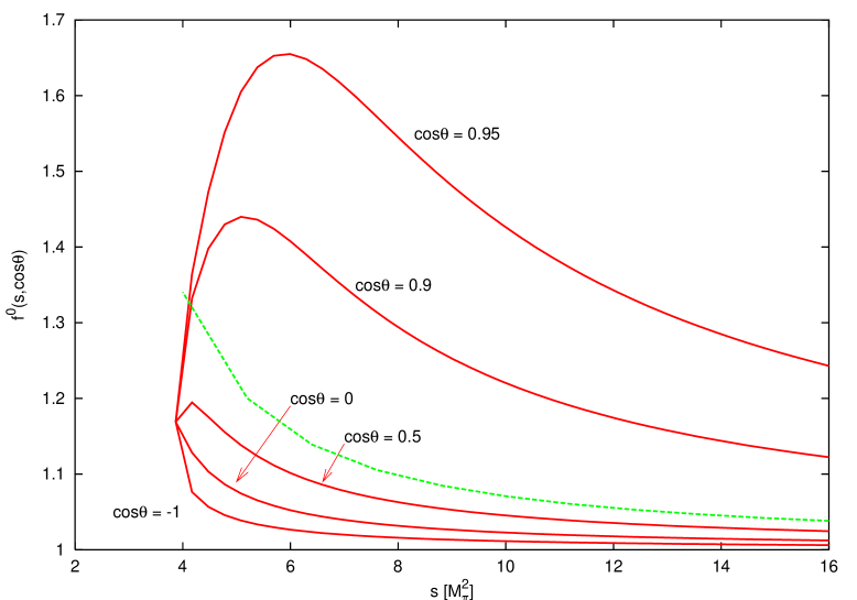
Figure 2: The lowest order amplitude $f^{(0)}(s,\cos\theta)$ including radiative corrections as a function of $s$ and for various values of the center-of-mass scattering angle $\theta$. The dashed curve shows the corresponding relative increase in the cross-section $\sigma$.

Although the value $t=0$ is excluded from the physical region of the reaction $\gamma\pi^{\pm}\to\pi^{0}\pi^{\pm}$, small values of $t$ are possible, and actually not only in the threshold region. Neglecting the pion mass difference for the time being, the threshold value is $f^{(0)}(4M_{\pi^{\pm}}^{2},\cos\theta)=1+(\alpha/\pi)(4\pi F_{\pi}/M_{\pi^{\pm}})^{2}=1.16$. Furthermore, in the forward direction, $|t|$ decreases as $s$ grows. The behaviour of $f^{(0)}(s,\cos\theta)$ in the range of $s$ covered by the Serpukhov experiment [6] is shown in Fig. 2. The increase in $f^{(0)}(s,\cos\theta)$, as compared to the constant value $f^{(0)}(s,\cos\theta)=1$ corresponding to the absence of isospin breaking, stays substantial for $\cos\theta\mathrel{\raise 2.58334pt\hbox{$>$}\kern-7.7778pt\lower 2.79857pt\hbox{$\sim$}}0.8$ even away from threshold, and by itself increases the total cross-section ${\sigma^{\rm\mbox{\tiny}{total}}}/{\mbox{Z}^{2}}$ by 16%, from 0.92 nb to 1.07 nb. In order to establish the robustness of this result, we next compute the radiative corrections to $f^{(1)}(s,\cos\theta)$ as well.

2.2 Electromagnetic corrections in $f^{(1)}(s,\cos\theta)$

The evaluation of the next-to-leading contribution $f^{(1)}(s,\cos\theta)$ involves loop diagrams with exactly one vertex from ${\cal L}_{(4)}^{-}$, and tree graphs, which involve the various counterterms. In the even intrinsic sector, the counterterms consist of the strong interaction low-energy constants $l_{i}$ of Ref. [8], and of the electromagnetic constants $k_{i}$ [16, 22], corresponding to the decomposition (there are also ${\cal O}(e^{4})$ counterterms, but we shall not consider radiative corrections of this order)

$${\cal L}^{+}_{(4)}={\cal L}^{+}_{\mbox{\tiny p}^{4}}+{\cal L}^{+}_{e^{2}\mbox{\tiny p}^{2}}\,.\\$$ (2.8)

In the odd intrinsic parity sector, the next-to-leading order Lagrangian has a similar decomposition

$${\cal L}^{-}_{(6)}={\cal L}^{-}_{\mbox{ \tiny e p}^{5}}+{\cal L}^{-}_{\mbox{\tiny e}^{3}\mbox{\tiny p}^{3}}\,.\\$$ (2.9)

The expression of ${\cal L}^{-}_{\mbox{\tiny e p}^{5}}$, which involves a set of counterterms $A_{i}$, has been worked out in Ref. [23], and we do not reproduce it here for the sake of brevity. The remaining term ${\cal L}^{-}_{\mbox{\tiny e}^{3}\mbox{\tiny p}^{3}}$ contains the ${\cal O}(e^{2})$ electromagnetic counterterms contributing to the anomalous sector. To our knowledge, they have not been classified so far. For the time being, we shall collect the full contribution of all electromagnetic counterterms in the anomalous sector in an “effective” low-energy constant $B_{\mbox{\tiny eff}}$.

In computing the loop graphs, we shall encounter ultraviolet divergences. These will be regularized within the same dimensional regularization scheme as used in Ref. [8]. The elimination of the divergences proceeds through the renormalization of the counterterms. The renormalized low-energy constants $l_{i}^{r}$, $k_{i}^{r}$, $A_{i}^{r}$ and $B_{\mbox{\tiny eff}}^{r}$ then depend on the renormalization scale $\mu$. As far as the contributions from the low-energy constants $l_{i}$ and $k_{i}$ are concerned, we express them in terms of the scale invariant quantities ${\bar{l}}_{i}$ and ${\bar{k}}_{i}$, as defined in Refs. [8] and [16], respectively. Of course, the final expression of $f^{(1)}(s,\cos\theta)$ has to be $\mu$-independent. We shall briefly address this issue at the end of this section.

In order to present our results we have found it convenient to split the expression of $f^{(1)}(s,\cos\theta)$ into three components,

$$f^{(1)}(s,\cos\theta)\,=\,f^{(1)}_{\mbox{\tiny QCD}}(s,\cos\theta)\,+\,f^{(1)}_{\mbox{\tiny FF}}(s,\cos\theta)\,+\,f^{(1)}_{\mbox{\tiny IRD}}(s,\cos\theta)\,,\\$$ (2.10)

which we shall describe in turn. The contribution $f^{(1)}_{\mbox{\tiny QCD}}(s,\cos\theta)$ contains the diagrams with only mesons in the loop, as well as the counterterms $A_{i}$. It amounts to the calculation of Ref. [9], except that one has to include effects of the the pion mass difference in the loops,

$$f^{(1)}_{\mbox{\tiny QCD}}(s,\cos\theta) = -\Big{\{}8M_{\pi^{0}}^{2}\Big{(}2A_{12}^{r}(\mu)-A_{13}^{r}(\mu)-A_{7}^{r}(\mu)+A_{8}^{r}(\mu)\Big{)}$$ (2.11)

$$-\frac{16}{3}\Delta_{\pi}\Big{(}A_{7}^{r}(\mu)-A_{8}^{r}(\mu)\Big{)}\Big{\}}-\frac{1}{96\pi^{2}F_{\pi}^{2}}\Big{\{}M_{\pi^{0}}^{2}+\,\frac{2}{3}\,\Delta_{\pi}$$

$$+(t+5M_{\pi^{0}}^{2}+2\Delta_{\pi})(\,\frac{M_{\pi^{0}}^{2}}{\Delta_{\pi}}\,\ln\frac{M_{\pi^{\pm}}^{2}}{M_{\pi^{0}}}-1)+3M_{\pi^{0}}^{2}\ln\frac{M_{\pi^{0}}^{2}}{\mu^{2}}\,\Big{\}}$$

$$+\frac{1}{6F_{\pi}^{2}}{\bar{J}}_{+-}(t)(t-4M_{\pi^{\pm}}^{2})$$

$$+\frac{1}{6F_{\pi}^{2}}{\bar{J}}_{+0}(u)\Big{\{}u-2(M_{\pi^{\pm}}^{2}+M_{\pi^{0}}^{2})+\frac{\Delta_{\pi}^{2}}{u}\Big{\}}$$

$$+\frac{1}{6F_{\pi}^{2}}{\bar{J}}_{+0}(s)\Big{\{}s-2(M_{\pi^{\pm}}^{2}+M_{\pi^{0}}^{2})+\frac{\Delta_{\pi}^{2}}{s}\Big{\}}\,,$$

where $\Delta_{\pi}=M_{\pi^{\pm}}^{2}-M_{\pi^{0}}^{2}$. ${\bar{J}}_{PQ}(s)$ is the scalar two-point function subtracted at $s=0$ [8] (the subscript identifies the charges, and hence the masses, of the two pions in the loop), and the terms $A_{i}^{r}(\mu)$ are the renormalized, scale-dependent counterterms from the anomalous ${\cal L}^{-}_{\rm\mbox{\tiny p}^{6}}$ Lagrangian. In practice, we shall only be interested in ${\cal O}(e^{2})$ corrections, neglecting contributions involving higher powers of $e^{2}$. Terms like $\Delta_{\pi}^{2}/s$ or $\Delta_{\pi}^{2}/u$ can therefore be omitted from the expression (2.11).

The second term, $f^{(1)}_{\mbox{\tiny FF}}(s,\cos\theta)$, arises from reducible diagrams with one photon propagator as in Fig. 1, where the blobs stand for form factors $F^{\pi}(0,t)$ and $F_{V}(t)$, computed at one-loop order,

$$f^{(1)}_{\mbox{\tiny FF}}(s,\cos\theta) = -2e^{2}\frac{1}{t}\Big{\{}\frac{1}{3}{\bar{J}}_{00}(t)(t-4M_{\pi^{0}}^{2})+\frac{t}{96\pi^{2}}\Big{(}{\bar{l}}_{6}-\ln\frac{M_{\pi^{0}}^{2}}{\mu^{2}}-\frac{2}{3}\Big{)}$$ (2.12)

$$-\frac{8}{3}\,F_{\pi}^{2}\Big{(}[A_{2}^{r}(\mu)-2A_{3}^{r}(\mu)-4A_{4}^{r}(\mu)]M_{\pi^{0}}^{2}-[A_{2}^{r}(\mu)-4A_{3}^{r}(\mu)]t\Big{)}\Big{\}}\,.$$

Again, ${\cal O}(e^{4})$ contributions have been neglected. Notice that two kinds of counterterms contribute: ${\bar{l}}_{6}$ has a non-anomalous origin and enters through the pion electromagnetic form factor $F_{V}(t)$, whereas the terms $A_{i}^{r}(\mu)$ belong to ${\cal L}^{-}_{\rm\mbox{\tiny ep}^{5}}$. If we add this contribution to $f^{(0)}(s,\cos\theta)$, we obtain, as expected,

$$F^{3\pi}_{0}[f^{(0)}(s,\cos\theta)\,+\,f^{(1)}_{\mbox{\tiny FF}}(s,\cos\theta)]\,=\,F^{3\pi}_{0}\,-\,2e\,\frac{F^{\pi}(0,t)F_{V}(t)}{t}\,,\\$$ (2.13)

with the one-loop expressions of the form factors given as

$$F^{\pi}(0,t) = F^{\pi}_{0}\Big{\{}1-\frac{8}{3}[A_{2}^{r}(\mu)-2A_{3}^{r}(\mu)-4A_{4}^{r}(\mu)]M_{\pi}^{2}$$

$$+\frac{8}{3}[A_{2}^{r}(\mu)-4A_{3}^{r}(\mu)-\frac{1}{256\pi^{2}}\ln\frac{M_{\pi^{0}}^{2}}{\mu^{2}}]t+\frac{1}{6F_{\pi}^{2}}{\bar{J}}_{00}(t)(t-4M_{\pi^{0}}^{2})\Big{\}}\,,$$

$$F_{V}(t) = 1+\frac{1}{6F_{\pi}^{2}}{\bar{J}}_{00}(t)(t-4M_{\pi^{0}}^{2})+\frac{t}{96\pi^{2}F_{\pi}^{2}}\,({\bar{l}}_{6}-\frac{2}{3})\,.$$ (2.14)

The last electromagnetic contribution, $f^{(1)}_{\mbox{\tiny IRD}}(s,\cos\theta)$, comes from irreducible diagrams, shown in Fig. 3, with a virtual photon in the loop. It is a ${\cal O}({\mbox{\rm e}}^{2})$ correction to the tree-level result (the contribution from one-loop radiative correction to the $\gamma$-$\pi^{+}$-$\pi^{-}$ vertex of Fig. 1, is omitted, being ${\cal O}({\mbox{\rm e}}^{4})$) and reads

$$f^{(1)}_{\mbox{\tiny IRD}}(s,\cos\theta)= e^{2}\Big{\{}\frac{1}{16\pi^{2}}\Big{[}-2+\frac{3M_{\pi^{0}}^{2}}{(s-M_{\pi^{0}}^{2})}+\frac{4M_{\pi^{0}}^{4}}{(s-M_{\pi^{0}}^{2})^{2}}-\log(\frac{m_{\gamma}^{2}}{M_{\pi^{0}}^{2}})$$ (2.15)

$$+\Big{(}\frac{3}{4}-2Z\Big{)}\ln\frac{M_{\pi^{0}}^{2}}{\mu^{2}}+\frac{Z}{6}({\bar{k}}_{1}-10{\bar{k}}_{2}-3{\bar{k}}_{4})+\frac{3}{8}(3{\bar{k}}_{1}-{\bar{k}}_{3})\Big{]}+B_{\mbox{\tiny eff}}^{r}(\mu)$$

$$+{\bar{J}}_{00}(s)\Big{[}1-\frac{M_{\pi^{0}}^{2}(M_{\pi^{0}}^{2}+s)}{(M_{\pi^{0}}^{2}-s)^{2}}\Big{]}+{\bar{J}}_{\gamma 0}(s)\Big{(}\frac{M_{\pi^{0}}^{2}+s}{M_{\pi^{0}}^{2}-s}\Big{)}$$

$$+(\frac{2t-4M_{\pi^{0}}^{2}}{t-4M_{\pi^{0}}^{2}})\Big{[}\frac{1}{8\pi^{2}}-{\bar{J}}_{00}(t)\Big{]}-(t-2M_{\pi^{0}}^{2})G_{+-\gamma}(t)$$

$$-2M_{\pi^{0}}^{2}H_{+-\gamma}(s;0)+H_{+-\gamma}(0;s)\frac{2M_{\pi^{0}}^{6}}{(M_{\pi^{0}}^{2}-s)^{2}}\Big{\}}$$

$$+e^{2}\Big{\{}(s\leftrightarrow u)\Big{\}}\,.$$

Notice the presence of a non-vanishing photon mass $m_{\gamma}$. It is needed to regulate the infrared divergence generated by the photon loop diagrams.

The functions $G_{+-0}(t)$ and $H_{+-0}(s;t)$ are related to the scalar three-point loop function $C_{0}$, defined as

$$C_{0}(M_{1}^{2},M_{2}^{2},M_{3}^{2};p_{1}^{2},p_{2}^{2},(p_{1}-p_{2})^{2})=\frac{1}{i}\int\frac{d^{d}\,q}{(2\pi)^{d}}\frac{1}{(q^{2}-M_{1}^{2})((q-p_{1})^{2}-M_{2}^{2})((q-p_{2})^{2}-M_{3}^{2})}\,,\\$$

through

$$G_{+-0}(t) = C_{0}(m_{\gamma}^{2},M_{\pi^{\pm}}^{2},M_{\pi^{\pm}}^{2};M_{\pi^{\pm}}^{2},M_{\pi^{\pm}}^{2},t)\,,$$

$$H_{+-0}(s;t) = C_{0}(0,M_{\pi^{\pm}}^{2},M_{\pi^{\pm}}^{2};M_{\pi^{\pm}}^{2},s,t)\,.$$ (2.16)

For $m_{\gamma}\to 0$, $G_{+-0}(t)$ can be expressed in terms of logarithms and dilogarithms. In the region of interest $t<0$, it is given by

$$G_{+-\gamma}(t)=-\frac{1}{32\pi^{2}s\beta_{t}}\Big{\{}4{\mbox{L}i}_{2}\left(\frac{1-\beta_{t}}{1+\beta_{t}}\right)+\ln^{2}\left(\frac{\beta_{t}-1}{\beta_{t}+1}\right)+\frac{\pi^{2}}{3}$$ (2.17)

$$\hskip 85.35826pt+2\Big{[}\ln\left(\frac{-t}{M_{\pi^{\pm}}^{2}}\right)-\ln\left(\frac{m_{\gamma}^{2}}{M_{\pi^{\pm}}^{2}}\right)+2\ln(\beta_{t})\Big{]}\,\ln\left(\frac{\beta_{t}-1}{\beta_{t}+1}\right)\Big{\}}\,,$$

where $\beta_{t}\equiv\beta(t)=\sqrt{1-{4M_{\pi^{\pm}}^{2}}/{t}}$.

The infrared divergences are handled as usual by considering the process with undetected soft photons, with energies less than the detector resolution $\Delta E$. At the present level of accuracy, one soft photon is enough, and an infrared finite observable is constructed by considering in addition the cross-section $\sigma^{\gamma}(s;\Delta E)$ for the process $\gamma\pi^{\pm}\to\pi^{0}\pi^{\pm}\gamma$. Then,

$$\frac{d\sigma+d\sigma^{\gamma}}{\sin^{3}\theta d\theta}\,\equiv\,(F^{3\pi}_{0})^{2}\,\big{\{}|f^{(0)}+f^{(1)}_{\mbox{\tiny QCD}}+f^{(2)_{\mbox{\tiny QCD}}}|^{2}\,+\,2{\mbox{Re}}[f^{(1)}_{\mbox{\tiny IRD}}]\,+\,2{\mbox{Re}}[f^{(1)}_{\mbox{\tiny FF}}]\,\big{\}}\,+\,\frac{d\sigma^{\gamma}}{\sin^{3}\theta d\theta}\,,\\$$ (2.18)

where we have also added the two-loop contribution $f^{(2)}_{\mbox{\tiny QCD}}$ without radiative corrections computed in Ref. [10], should be infrared finite. The expression for the last term is cumbersome [24] and we do not reproduce it here. We have checked that the infrared divergence appearing in the soft bremstrahlung term indeed cancels the one in $2{\mbox{Re}}[{f}^{(1)}_{\mbox{\tiny IRD}}]$.

2.3 Renormalization scale dependence of the counterterms

In order to establish that $f^{(1)}(s,\cos\theta)$ indeed does not depend on the renormalization scale $\mu$, we need to know the scale dependence of the various counterterms involved in the expressions (2.11), (2.12) and (2.15). This information has been obtained independently, using functional techniques, for the low-energy constants $l_{i}^{r}(\mu)$ [8] and $k_{i}^{r}(\mu)$ [16, 22], but not for the remaining ones. On the other hand, we may however use our present results in order to pin down the scale dependence of several combinations of the renormalized constants $A^{r}_{i}(\mu)$ and of $B^{r}_{\mbox{\tiny eff}}(\mu)$. For instance, the form factor $F^{\pi}(0,t)$ (2.14), being an observable quantity, must be scale independent by itself, which implies

$$\mu\,\frac{d}{d\mu}\,[A_{2}^{r}(\mu)-2A_{3}^{r}(\mu)-4A_{4}^{r}(\mu)]\,=\,0\,,$$

$$\mu\,\frac{d}{d\mu}\,[A_{2}^{r}(\mu)-4A_{3}^{r}(\mu)]\,=\,-\,\frac{1}{128\pi^{2}F_{\pi}^{2}}\,.$$ (2.19)

Furthermore, the scale invariance of the amplitudes for $\gamma\gamma\to\pi^{0}\pi^{0}\pi^{0}$ and $\gamma\gamma\to\pi^{+}\pi^{-}\pi^{0}$ require in addition that [26]

$$\mu\,\frac{d}{d\mu}\,[A_{7}^{r}(\mu)-A_{8}^{r}(\mu)+2A_{12}^{r}(\mu)-A_{13}^{r}(\mu)]\,=\,-\,\frac{1}{128\pi^{2}F_{\pi}^{2}}\,.\\$$ (2.20)

Then, the condition that $f^{(1)}(s,\cos\theta)$ does not depend on the renormalization scale $\mu$ amounts to

$$\mu\,\frac{d}{d\mu}\,[A_{7}^{r}(\mu)-A_{8}^{r}(\mu)] = -\,\frac{3}{128\pi^{2}F_{\pi}^{2}}\,,$$

$$\mu\,\frac{dB^{r}_{\mbox{\tiny eff}}(\mu)}{d\mu} = \frac{3}{32\pi^{2}}\,.$$ (2.21)

Having discussed the scale dependence of the low-energy constants, it still remains to pin down their values in order to proceed.

3 Counterterm estimates and numerical results

In this section, we shall first provide estimates for the various counterterm combinations that appear in $f^{(1)}(s,\cos\theta)$. We then convert our computation into numerical results for the experimental observables discussed in section 1.

3.1 Counterterm estimates

The low-energy constant $\bar{l}_{6}$ contributes to the slope of the electromagnetic form factor of the pion [8] and its value is well determined, $\bar{l}_{6}=16.0\pm 0.5\pm 0.7\,$ [27]. The combinations of constants $A_{i}$ which describe the ${\cal O}(M_{\pi}^{2})$ corrections to $F^{\pi}(0,0)$ (2.14) and the slope of $F^{\pi}(0,t)$ were estimated by studying the $\langle VVP\rangle$ QCD three-point correlator [28, 26, 29]. We shall use the estimates of Ref. [29] (hereafter we set $\mu=M_{\rho}$)

$$-\frac{8}{3}(A^{r}_{2}-2A^{r}_{3}-4A^{r}_{4})M_{\pi^{0}}^{2} = (-6\pm 2)\times 10^{-3}\,,$$

$$\frac{8}{3}(A^{r}_{2}-4A^{r}_{3})M_{\pi^{0}}^{2} = (+26\pm 9)\times 10^{-3}\,.$$ (3.1)

A similar treatment of the combination of $A_{i}$’s appearing in $f^{(1)}_{\mbox{\tiny QCD}}$ would, for instance, require a detailed analysis of the $\langle VPPP\rangle$ four-point function along the lines of Ref. [29], which is lacking at the moment. If we assume naive resonance saturation by the lightest vectors, axials, pseudoscalars and scalars, only vectors contribute to the QCD part. We obtain the rough estimate

$$-\Big{\{}8M_{\pi^{0}}^{2}(2A^{r}_{12}-A^{r}_{13})-\frac{8}{3}(M_{\pi^{0}}^{2}+2M_{\pi^{\pm}}^{2})(A^{r}_{7}-A^{r}_{8})\Big{\}}\sim\frac{2M_{\pi^{\pm}}^{2}+M_{\pi^{0}}^{2}}{2M_{\rho}^{2}}.\\$$ (3.2)

The $\bar{k}_{i}$ constants appearing in Eq. (2.15) are the finite, scale independent contributions of the electromagnetic counterterms $k_{i}$. The precise relations among the non-renormalized $k_{i}$, the scale dependent renormalized $k_{i}^{r}(\mu)$ and the scale independent $\bar{k}_{i}$ have been worked out by several authors [22, 16]. In [16], the following estimates, based on naive dimensional analysis, were given

$$\bar{k}_{1}=3.6\pm 1.3\,,\qquad\bar{k}_{2}=3.5\pm 1.3\,,\qquad\bar{k}_{3}=3.4\pm 0.7\,,\qquad\bar{k}_{4}=3.5\pm 1.3\,.\\$$ (3.3)

Finally, there remains the effective anomalous electromagnetic counterterm $B_{\mbox{\tiny eff}}^{r}(\mu)$ in the anomalous sector, for which naive dimensional analysis gives

$$|\,B^{r}_{\mbox{\tiny eff}}(\mu)|\,\mathrel{\raise 2.58334pt\hbox{$<$}\kern-7.7778pt\lower 2.79857pt\hbox{$\sim$}}\frac{1}{16\pi^{2}}\,.\\$$ (3.4)

3.2 Numerical results

Most of the existing results in the literature share a moderate increase of the amplitude $F^{3\pi}(s,\cos\theta)$ with $s$, and a very small sensitivity to $\cos\theta$. This is, in particular, the case for the ChPT results, both at one and two-loop order. When electromagnetic corrections are taken into account, two effects must be considered. First, a different mass for the neutral and charged pion modifies the lower limit of the phase-space integral in Eq. (1.8). This represents small changes, an increase of $\sim 6\%$ in the Primakov cross section $\sigma^{\mbox{\tiny total}}/{\mbox{Z}}^{2}$, a decrease of $\sim 4\%$ in $F^{3\pi}_{0,\,{\mbox{\tiny exp}}}$, which goes into the right direction, but still does not match the theoretical value. Second, the radiatively corrected expression of Eq. (2.18) should be used in evaluating Eq. (1.8). In order to see how much the two combined effects modify the experimental determination of $F^{3\pi}_{0,\,{\mbox{\tiny exp}}}$, we show in Table 1 the values obtained for $F^{3\pi}_{0}$ from the experimental result of Ref. [6], using the expressions for the amplitude $F^{3\pi}(s,\cos\theta)$ at different orders of ChPT in the $M_{\pi^{0}}=M_{\pi^{\pm}}$ isospin limit (first line), and the corresponding values when ${\cal O}$(e${}^{2})$ electromagnetic corrections are included at one loop (second line). As numerical input parameters we have used [5] $M_{\pi^{\pm}}=139.570~{}\mbox{MeV}\,,M_{\pi^{0}}=134.976~{}\mbox{MeV}\,,F_{\pi^{\pm}}=92.4~{}\mbox{MeV}\,.$ In addition, an energy resolution for undetected photons of $\Delta E=10$ MeV has been chosen. We have checked that the final results are very insensitive to the actual value used for $\Delta E$ (we took values up to 50 MeV) and for the next-to-leading order counterterms. The errors shown in Table 1 have been computed adding the statistical and systematic experimental errors in Eq. (1.7).

It is interesting to observe that the electromagnetic corrections are sizeable: they represent an increase of $\sim 0.15$ nb in the Primakov cross-section $\sigma^{\mbox{\tiny total}}/{\mbox{Z}}^{2}$, bringing the theoretical prediction to the value

$$\sigma^{\mbox{\tiny total}}_{\mbox{\tiny th}}/{\mbox{Z}}^{2}\,=\,1.33\ \pm 0.03\ {\mbox{nb}}\,,\\$$ (3.5)

where the error has been estimated using higher order corrections via the non-perturbative chiral approach of Ref. [10]. This value of the cross-section corresponds to

$${\overline{F}}^{\,3\pi}_{\mbox{\tiny th}}\,=\,11.7\ \pm 0.2\ {\mbox{GeV}}^{-3}\\$$ (3.6)

for the average amplitude ${\overline{F}}^{\,3\pi}$. Equivalently, if we keep $F^{3\pi}_{0}$ as a free parameter, and insert the theoretical expression (2.18) into Eqs. (1.8) and (LABEL:cross), the experimental determination becomes

$$F^{3\pi}_{0,\,{\mbox{\tiny exp}}}\,=\,10.7\pm 1.2\ {\mbox{GeV}}^{-3}\,,\\$$ (3.7)

much lower than the value (1.12) obtained if radiative corrections are omitted, and compatible with the theoretical value $F^{3\pi}_{0}=(9.72\pm 0.09)\ {\mbox{GeV}}^{-3}$. Interestingly enough, the contribution of the electromagnetic corrections to the amplitude $F^{3\pi}(s,\cos\theta)$ is larger than the genuine chiral corrections. This can be observed in Fig. 4, where we plot the squared amplitude, as a function of $s$, for the ${\cal O}(\rm\mbox{p}^{8})$ result, including radiative corrections at one loop, for several values of $\cos\theta$ (curves). We also include a shaded area for the same result without electromagnetic corrections, covering the full range of $\cos\theta$. While the latter is almost insensitive to $\cos\theta$ and slowly raises with $s$, the former shows a richer structure, with substantially large contributions for $\cos\theta$ approaching $1$.

This is in contrast with most other mesonic processes studied so far in ChPT, where electromagnetic corrections in general give reasonably small contributions. The reason for this difference lies in a peculiarity of the $\gamma\pi^{\pm}\to\pi^{0}\pi^{\pm}$ process, which admits a kinematically enhanced contribution, due to the $t$-channel exchange of a single photon, and which actually completely dominates the radiative corrections. As a matter of fact, our results can be very well reproduced by adding only the “universal” contribution coming from the pole in Fig. 1 to the one and two-loop chiral corrections,

$$\frac{d\sigma}{\sin^{3}\theta d\theta}\,=\,(F^{3\pi}_{0})^{2}\,|1-2e^{2}\,\frac{F_{\pi}^{2}}{t}+f^{(1)}_{\mbox{\tiny QCD}}+f^{(2)}_{\mbox{\tiny QCD}}|^{2}\,.\\$$ (3.8)

The situation in this respect would have been different in the case of the crossed channel $\gamma\pi^{0}\to\pi^{+}\pi^{-}$. There, the photon-exchange pole appears in the $s$-channel. With a minimum value of $4M_{\pi^{\pm}}^{2}$ for $s$, the net effect is mild, at the few-percent level.

4 Conclusions

In the present work, we have considered, within the framework of one-loop ChPT, ${\cal O}(e^{2})$ radiative corrections to the process $\gamma\pi^{\pm}\to\pi^{0}\pi^{\pm}$. They turn out to be quite sizeable, being larger than the genuine two-loop chiral corrections computed in Ref. [10], and increase the two-loop theoretical value for the Primakov cross-section measured in Ref. [6] by $~{}\sim 0.15$ nb. Such a large effect originates mainly from a one-photon exchange contribution in the $t$-channel. Since small kinematical values for $t$ are allowed, one obtains large contributions to the cross-section. Other electromagnetic contributions are very small. These corrections are therefore very stable against variations of the counterterms that enter at next-to-leading ${\cal O}$(e²p${}^{2})$. The inclusion of radiative corrections brings theory and experiment into agreement. Future high precision experiments [17, 18, 19] will hopefully improve this agreement and test the rôle of electromagnetic corrections. In this respect, it would be worthwhile to investigate the experimental possibilities to study, in addition, the reaction $\gamma\pi^{0}\to\pi^{+}\pi^{-}$, through e.g. the process $\gamma p\to\pi^{+}\pi^{-}p$, where no such important electromagnetic effects are expected.

Acknowledgments
We thank A. Bramon, R. Escribano and J. Stern for clarifying discussions. This work was supported in part by TMR, EC–Contract No. ERBFMRX–CT980169 (EURODAPHNE).

Table 1: Different chiral determinations of $F^{3\pi}_{0,\,{\mbox{\tiny exp}}}$ extracted from Eqs. (1.8) and (LABEL:cross), as explained in the main text. The numbers in the first line correspond to the ${\cal O}(\rm\mbox{p}^{4})$ tree-level, next-to-leading ${\cal O}(\rm\mbox{p}^{6})$ [9] and the dispersive treatment at ${\cal O}(\rm\mbox{p}^{8})$ [10]. The second line correspond to the same results when electromagnetic corrections at ${\cal O}(\rm\mbox{e}^{2})$ are included. All results are in units of GeV^-3. These values should be compared with the theoretical prediction $F^{3\pi}_{0}=9.72\pm 0.09$ GeV^-3.

	${\cal O}(\rm\mbox{p}^{4})$	${\cal O}(\rm\mbox{p}^{6})$	${\cal O}(\rm\mbox{p}^{8})$
$F^{3\pi}_{0,\,{\mbox{\tiny exp}}}(e=0)$	$12.9\pm 1.4$	$11.9\pm 1.3$	$11.4\pm 1.3$
$F^{3\pi}_{0,\,{\mbox{\tiny exp}}}(e\neq 0)$	$12.0\pm 1.2$	$11.2\pm 1.2$	$10.7\pm 1.2$

Figure 1: Reducible one photon exchange diagram contributing to $F^{3\pi}(s,\cos\theta)$ via the electromagnetic form factor of the pion and the anomalous $\pi^{0}\rightarrow\gamma\gamma^{*}$ form factor $F^{\pi}(0,t)$.

Figure 3: One-loop diagrams contributing to $\gamma\to\pi\pi\pi$ via photon loops.

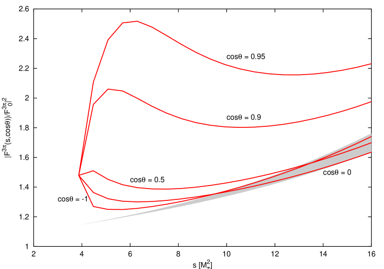
Figure 4: The scattering amplitude $|{F}^{3\pi}(s,\cos\theta)|^{2}$ vs. s (in units of $M_{\pi}^{2}$) for several values of $\cos\theta$ at ${\cal O}$(p${}^{8})$ with (curves) and without (shaded area) radiative corrections. The shaded area covers the full range of $\cos\theta$.

References

- [1] M.V. Terent’ev, JETP Letters 14, 94 (1971) [Zh. Eksp. Teor. Fiz. Pis’ma 14, 140 (1971)]; Phys. Lett. 38B, 419 (1972).
- [2] S.L. Adler, B.W. Lee, S.B. Treiman, and A. Zee, Phys. Rev. D 4, 3497 (1971).
-
[3]
J. Wess and B. Zumino,
Phys. Lett. 37B (1971) 95.
E. Witten, Nucl. Phys. B 223, 422 (1983). - [4] R. Aviv and A. Zee, Phys. Rev. D 5, 2372 (1972).
- [5] Particle Data Group, D.E. Groom et al, Eur. Phys. J. C 15, 1 (2000).
- [6] Y. M. Antipov et al., Phys. Rev. D 36, 21 (1987).
- [7] S. Weinberg, Physica A 96, 327 (1979).
- [8] J. Gasser and H. Leutwyler, Phys. Lett. B 125, 321 (1983); Ann. Phys. 158, 142 (1984).
- [9] J. Bijnens, A. Bramon and F. Cornet, Phys. Lett. B 237, 488 (1990).
- [10] T. Hannah, Nucl. Phys. B 593, 577 (2001) [hep-ph/0102213].
-
[11]
D. Klabucar and B. Bistrovic,
hep-ph/0012273;
hep-ph/0009259;
Phys. Lett. B 478, 127 (2000)
[hep-ph/9912452];
Phys. Rev. D 61, 033006 (2000)
[hep-ph/9907515].
X. Li and Y. Liao, Phys. Lett. B 505, 119 (2001) [hep-ph/0101214].
R. Alkofer and C. D. Roberts, Phys. Lett. B 369, 101 (1996) [hep-ph/9510284].
M. A. Ivanov and T. Mizutani, Phys. Rev. D 53, 1470 (1996) [hep-ph/9506479]. - [12] S. Rudaz, Phys. Lett. 145B, 281 (1984).
- [13] T. D. Cohen, Phys. Lett. B 233, 467 (1989).
- [14] B. R. Holstein, Phys. Rev. D 53, 4099 (1996) [hep-ph/9512338].
- [15] T. N. Truong, hep-ph/0105123.
- [16] M. Knecht and R. Urech, Nucl. Phys. B 519, 329 (1998) [hep-ph/9709348].
- [17] R. A. Miskimen, K. Wang and A. Yegneswaran, CEBAF proposal PR-94-015, 1994; available from the URL http://www.jlab.org/exp_prog/experiments/summaries/E94-015.ps
- [18] M. A. Moinester, V. Steiner and S. Prakhov, Hadron photon interactions in COMPASS, hep-ex/9903017.
- [19] M. A. Moinester et al. [SELEX Collaboration], Inelastic electron pion scattering at FNAL (SELEX), hep-ex/9903039.
- [20] R. Urech, Nucl. Phys. B 433, 234 (1995) [hep-ph/9405341].
- [21] H. Neufeld and H. Rupertsberger, Z. Phys. C 68, 91 (1995); H. Neufeld and H. Rupertsberger, Z. Phys. C 71, 131 (1996) [hep-ph/9506448].
- [22] U. Meissner, G. Müller and S. Steininger, Phys. Lett. B 406, 154 (1997) [Erratum-ibid. B 407, 454 (1997)] [hep-ph/9704377].
- [23] H. W. Fearing and S. Scherer, Phys. Rev. D 53, 315 (1996) [hep-ph/9408346].
- [24] M. Vanderhaeghen, J. M. Friedrich, D. Lhuillier, D. Marchand, L. Van Hoorebeke and J. Van de Wiele, Phys. Rev. C 62 (2000) 025501 [hep-ph/0001100].
-
[25]
D. Issler, Report-no SLAC-PUB-4943 (1989; revised 1990).
R. Akhoury and A. Alfakih, Annals Phys. 210, 81 (1991).
J. F. Donoghue and D. Wyler, Nucl. Phys. B 316, 289 (1989).
J. Bijnens, A. Bramon and F. Cornet, Z. Phys. C 46, 599 (1990). - [26] Ll. Ametller, J. Kambor, M. Knecht and P. Talavera, Phys. Rev. D 60, 094003 (1999) [hep-ph/9904452].
- [27] J. Bijnens, G. Colangelo and P. Talavera, JHEP 05, 014 (1998) [hep-ph/9805389].
- [28] B. Moussallam, Phys. Rev. D 51, 4939 (1995) [hep-ph/9407402].
- [29] M. Knecht and A. Nyffeler, Resonance estimates of low-energy constants and QCD short-distance constraints, hep-ph/0106034. (To appear in Eur. Phys. J. C.)