FSU-HEP-2001-0601

BNL-HET-01/20

hep-ph/0107101

Next-to-Leading Order Results

for $t{\overline{t}}h$ Production at the Tevatron

L. Reina
Physics Department, Florida State University,
Tallahassee, FL 32306, USA

S. Dawson
Physics Department, Brookhaven National Laboratory,
Upton, NY 11973, USA

We compute the ${\cal O}(\alpha_{s}^{3})$ total cross section for the process $p{\overline{p}}\rightarrow t{\overline{t}}h$ in the Standard Model, at $\sqrt{s_{H}}\!=\!2$ TeV. The next-to-leading order corrections drastically reduce the renormalization and factorization scale dependence of the Born cross section and slightly decrease the total cross section for renormalization and factorization scales between $m_{t}$ and $2m_{t}$.

Abstract

We compute the ${\cal O}(\alpha_{s}^{3})$ total cross section for the process $p{\overline{p}}\rightarrow t{\overline{t}}h$ in the Standard Model, at $\sqrt{s_{H}}\!=\!2$ TeV. The next-to-leading order corrections drastically reduce the renormalization and factorization scale dependence of the Born cross section and slightly decrease the total cross section for renormalization and factorization scales between $m_{t}$ and $2m_{t}$.

1. Among the most important goals of present and future colliders is the study of the electroweak symmetry breaking mechanism and the origin of fermion masses. If the introduction of one or more Higgs fields is responsible for the breaking of the electroweak symmetry, then at least one Higgs boson should be relatively light, and certainly in the range of energies of present (Tevatron) or future (LHC) hadron colliders. The present lower bounds on the Higgs mass have been set by LEP to be $M_{h}\!>\!113.5$ GeV [1] for the Standard Model (SM) Higgs boson ($h$), and $M_{h^{0},A^{0}}\!>\!91$ GeV [2] for the light scalar ($h^{0}$) and pseudoscalar ($A^{0}$) Higgs bosons of the minimal supersymmetric standard model (MSSM). At the same time, precision fits to SM results indirectly point to the existence of a light Higgs boson, $M_{h}\!<\!212-236$ GeV [3], while the MSSM requires the existence of a scalar Higgs boson lighter than about $130$ GeV [4]. Therefore, the possibility of a Higgs boson discovery in the mass range around $115-130$ GeV seems increasingly likely.

In this context, the Tevatron will play a crucial role and will have the opportunity to discover a Higgs boson in the mass range between the experimental lower bound and about 180 GeV [5]. The dominant Higgs production modes at the Tevatron are gluon-gluon fusion, $gg\rightarrow h$, and the associated production with a weak boson, $q{\overline{q}}\rightarrow Wh,~{}Zh$ . Because of small event rates and large backgrounds, the Higgs search in these channels can be problematic, requiring the highest possible luminosity. It is therefore necessary to investigate all possible production channels, in the effort to fully exploit the range of opportunities offered by the available statistics.

Recently, attention has been drawn to the possibility of detecting a Higgs signal in association with a pair of top-antitop quarks, i.e. in $p{\overline{p}}\rightarrow t{\overline{t}}h$ [6]. This production mode can play a role almost over the entire Higgs mass range accessible at the Tevatron. Although it has a small event rate, $\sim 1-5$ fb for a SM like Higgs, the signature ($W^{+}W^{-}b{\overline{b}}b{\overline{b}}$) is quite spectacular. Furthermore, at the Tevatron (unlike at the LHC), the signal and background for this process have quite different shapes. The statistics are too low to allow any direct measurement of the top Yukawa couplings, but recent studies [7] indicate that this channel can reduce the luminosity required for a Higgs discovery at Run II of the Tevatron by as much as 15-20%.

Up to now the cross section for $p\bar{p}\rightarrow t\bar{t}h$ has been known only at tree level. As for any other hadronic process, first order QCD corrections are expected to be important and are crucial in order to reduce the dependence of the cross section on the renormalization and factorization scales. In this letter we present the results of our calculation of the NLO QCD corrections to the total cross section for $p{\overline{p}}\rightarrow t{\overline{t}}h$ in the Standard Model, at the Tevatron. A detailed review of the calculation will be presented elsewhere [8]. We find good agreement with the analogous results presented in Ref. [9].

2. The total cross section for $p{\overline{p}}\rightarrow t{\overline{t}}h$ at ${\cal O}(\alpha_{s}^{3})$ can be written as:

$$\sigma(p{\overline{p}}\rightarrow t{\overline{t}}h)_{NLO} = \sum_{ij}\int dx_{1}dx_{2}{\cal F}_{i}^{p}(x_{1},\mu){\cal F}_{j}^{{\overline{p}}}(x_{2},\mu)$$ (2)

$$~{}~{}~{}~{}\cdot{\hat{\sigma}}^{ij}_{NLO}(x_{1},x_{2},\mu)\,\,\,,$$

where ${\cal F}_{i}^{p,{\overline{p}}}$ are the NLO parton distribution functions for parton $i$ in a proton/antiproton, defined at a generic factorization scale $\mu_{f}\!=\!\mu$, and ${\hat{\sigma}}^{ij}_{NLO}$ is the ${\cal O}(\alpha_{s}^{3})$ parton level total cross section for incoming partons $i$ and $j$, made of the two channels $q\bar{q},\,gg\rightarrow t\bar{t}h$, and renormalized at an arbitrary scale $\mu_{r}$ which we also take to be $\mu_{r}\!=\!\mu$. At the Tevatron, for $p{\overline{p}}$ collisions at hadronic center of mass energy $\sqrt{s_{H}}\!=\!2$ TeV, more than $90\%$ of the tree level total cross section comes from $q{\overline{q}}\rightarrow t{\overline{t}}h$, summed over all light quark flavors. Therefore, we compute $\sigma(p{\overline{p}}\rightarrow t{\overline{t}}h)_{NLO}$ by including in ${\hat{\sigma}}^{ij}_{NLO}$ only the ${\cal O}(\alpha_{s})$ corrections to $q{\overline{q}}\rightarrow t{\overline{t}}h$. The calculation of $gg\rightarrow t{\overline{t}}h$ at ${\cal O}(\alpha_{s}^{3})$ is, however, crucial to determine $\sigma_{NLO}(pp\rightarrow t{\overline{t}}h)$ for the LHC, since in $pp$ collisions at $\sqrt{s_{H}}\!=\!14$ TeV a large fraction of the total cross section comes from the $gg\rightarrow t{\overline{t}}h$ channel. The ${\cal O}(\alpha_{s}^{3})$ total cross section for the LHC has been estimated within the Effective Higgs Approximation in Ref. [10]. Full results are presented in Ref. [9] and will also appear in Ref. [11].

We write the ${\cal O}(\alpha_{s}^{3})$ parton level total cross section as:

$${\hat{\sigma}}_{NLO}^{ij}(x_{1},x_{2},\mu)=$$ (3)

$$=\alpha_{s}^{2}(\mu)\biggl{\{}{\hat{f}}_{LO}^{ij}(x_{1},x_{2})+{\alpha_{s}(\mu)\over 4\pi}{\hat{f}}_{NLO}^{ij}(x_{1},x_{2},\mu)\biggr{\}}$$ (4)

$$\equiv{\hat{\sigma}}_{LO}^{ij}(x_{1},x_{2},\mu)+\delta{\hat{\sigma}}_{NLO}^{ij}(x_{1},x_{2},\mu)\,\,\,,$$ (5)

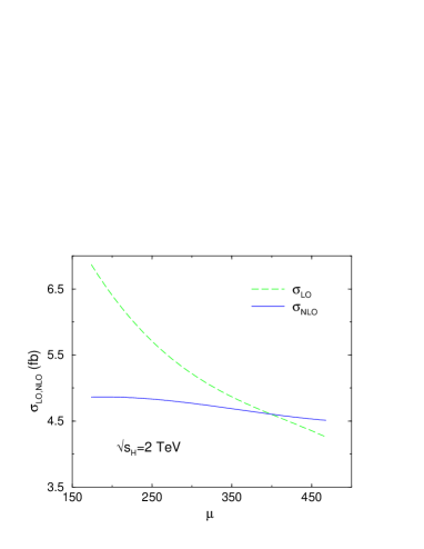
where $\alpha_{s}(\mu)$ is the strong coupling constant renormalized at the arbitrary scale $\mu_{r}\!=\!\mu$, ${\hat{\sigma}}_{LO}^{ij}(x_{1},x_{2},\mu)$ is the ${\cal O}(\alpha_{s}^{2})$ Born cross section, and $\delta{\hat{\sigma}}_{NLO}^{ij}(x_{1},x_{2},\mu)$ consists of the ${\cal O}(\alpha_{s})$ corrections to the Born cross section. The Born cross section ${\hat{\sigma}}_{LO}^{ij}(x_{1},x_{2},\mu)$ has a strong $\mu$-dependence, which is canceled at NLO by $\delta{\hat{\sigma}}_{NLO}^{ij}(x_{1},x_{2},\mu)$, up to term of ${\cal O}(\alpha_{s}^{4})$. The resulting NLO cross section is therefore much more stable under variations of $\mu$, as will be discussed in the following (see also Fig. 3).

$\delta{\hat{\sigma}}_{NLO}^{ij}(x_{1},x_{2},\mu)$ contains both virtual and real corrections to the lowest order cross section and can be written as the sum of two terms:

$$\delta{\hat{\sigma}}_{NLO}^{ij}(x_{1},x_{2},\mu) = \int d(PS_{3})M(ij\rightarrow t{\overline{t}}h)$$ (6)

$$+ \int d(PS_{4})M(ij\rightarrow t{\overline{t}}h+g)$$ (7)

$$= \sigma_{virt}+\sigma_{real}\,\,\,,$$ (8)

where $M(ij\rightarrow t\bar{t}h)$ and $M(ij\rightarrow t\bar{t}h+g)$ are respectively the matrix elements squared for the ${\cal O}(\alpha_{s}^{3})$ $2\rightarrow 3$ and $2\rightarrow 4$ processes averaged over the initial degrees of freedom and summed over the final ones, while $d(PS_{3})$ and $d(PS_{4})$ denote the integration over the corresponding three/four particle phase space. The first term represents the contribution of the virtual corrections, while the last one is due to the real gluon emission.

3. The ${\cal O}(\alpha_{s})$ virtual corrections to the tree level $q{\overline{q}}\rightarrow t{\overline{t}}h$ process consist of self-energy, vertex, box, and pentagon diagrams. The calculation of the virtual diagrams has been performed using dimensional regularization in $d\!=\!4-2\epsilon$ dimensions. The diagrams have been evaluated using FORM [12] and Maple, and all tensor integrals have been reduced to linear combinations of a fundamental set of scalar integrals. We have computed analytically all scalar integrals which give rise to either ultraviolet or infrared singularities, while finite scalar integrals have been evaluated using standard packages [13]. Among the integrals which have been computed analytically, many scalar box integrals and the scalar pentagon integrals are extremely laborious, due to the large number of massive particles present in the final state. Box and pentagon diagrams are ultraviolet finite, but have infrared divergences. These integrals are evaluated using the method of Ref. [14] and analytic results are presented in Ref. [8].

Self-energy and vertex diagrams contain both infrared and ultraviolet divergences. The ultraviolet divergences are renormalized by introducing a suitable set of counterterms. Since the cross section is a renormalization group invariant, we only need to renormalize the wave function of the external fields, the top quark mass, and the coupling constants. We use on-shell subtraction for the wave-function renormalization of the external fields. We define the top mass counterterm in such a way that $m_{t}$ is the pole mass. This counterterm must be used twice: once to renormalize the top quark mass, and again to renormalize the top quark Yukawa coupling. Finally, for $\alpha_{s}(\mu)$ we use the $\overline{MS}$ scheme, modified to decouple the top quark [15]. The first $n_{lf}$ light fermions are subtracted using the $\overline{MS}$ scheme, while the divergences associated with the heavy quark loop are subtracted at zero momentum.

4. The ${\cal O}(\alpha_{s})$ corrections to the Born cross section due to real gluon emission have been computed using a two cut-off implementation of the phase space slicing algorithm [16]. The contributions to $q{\overline{q}}\rightarrow t{\overline{t}}h+g$ are first divided into a soft and a hard contribution,

$$\sigma_{real}(q{\overline{q}}\rightarrow t{\overline{t}}h+g)=\sigma_{soft}+\sigma_{hard}\,\,\,,$$ (9)

where soft and hard refer to the energy of the radiated gluon. This division into hard and soft contributions depends on an arbitrary soft cut-off, $\delta_{s}$, such that the energy of the radiated gluon is considered soft if $E_{g}\leq\delta_{s}{\sqrt{s}\over 2}$. The cut-off $\delta_{s}$ must be very small, such that terms of order $\delta_{s}$ can be neglected. Therefore, to evaluate the soft contribution, the eikonal approximation to the matrix elements can be taken and the integral over the soft degrees of freedom performed analytically.

The hard contribution to $q{\overline{q}}\rightarrow t{\overline{t}}h+g$ is further divided into a hard/collinear and a hard/not collinear region. The hard/collinear region is defined as the region where the energy of the gluon is $E_{g}>\delta_{s}{\sqrt{s}\over 2}$ and the gluon is radiated from the initial massless quarks at an angle $\theta_{ig}$ ($i\!=\!q,\bar{q}$) such that $(1-\cos\theta_{gi})\leq\delta_{c}$, for an arbitrary small collinear cut-off $\delta_{c}$. The matrix element squared in the hard/collinear limit is found using the leading pole approximation and the integration over the angular degrees of freedom is performed analytically. The hard gluon emission from the final massive quarks never belongs to the hard/collinear region. The contribution from the hard/not collinear region is finite and is computed numerically.

$\sigma_{soft}$ and $\sigma_{hard/coll}$ contain IR singularities, which are calculated using dimensional regularization, and cancel exactly the analogous singularities from the virtual contributions, after absorbing mass singularities in the renormalized parton distribution functions.

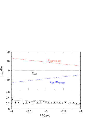
Both $\sigma_{soft}$ and $\sigma_{hard}$ depend on the two arbitrary cut-offs $\delta_{s}$ and $\delta_{c}$, but their sum, i.e. the physical cross section, is cut-off independent. In Figs. 1, we show the dependence of $\sigma_{real}$ on the soft cut-off, $\delta_{s}$, for a fixed value of the hard/collinear cut-off, $\delta_{c}\!=\!10^{-4}$. In the upper window we illustrate the cancellation of the $\delta_{s}$ dependence between $\sigma_{soft}+\sigma_{hard/coll}$ and $\sigma_{hard/non-coll}$, while in the lower window we show $\sigma_{real}$ with the statistical errors from the Monte Carlo integration. For $\delta_{s}$ in the range $10^{-4}-10^{-2}$, a clear plateau is reached and the result is independent of $\delta_{s}$. We point out that Fig. 1 only shows distributions of the form $d\sigma/d\delta_{s}$, so the corresponding cross sections are in this case twice the values that can be read from the plot. Analogously, Fig. 2 shows the independence of $\sigma_{real}$ on the hard/collinear cut-off, $\delta_{c}$. All the results presented in the following are obtained using $\delta_{s}$ and $\delta_{c}$ of order $10^{-3}$.

FIG. 1.: Dependence of $\sigma_{real}(p{\overline{p}}\rightarrow t{\overline{t}}h)$ on the soft cut-off $\delta_{s}$, at $\sqrt{s_{H}}\!=\!2$ TeV, for $M_{h}\!=\!120$ GeV, $\mu\!=\!m_{t}$, and $\delta_{c}=10^{-4}$. The lower scale shows the statistical error on $\sigma_{real}$.

FIG. 2.: Dependence of $\sigma_{real}(p{\overline{p}}\rightarrow t{\overline{t}}h)$ on the collinear cut-off $\delta_{c}$, at $\sqrt{s_{H}}\!=\!2$ TeV, for $M_{h}\!=\!120$ GeV, $\mu\!=\!m_{t}$, and $\delta_{s}\!=\!0.005$. The lower scale shows the statistical error on $\sigma_{real}$.

5. Our numerical results are found using CTEQ4M parton distribution functions for the calculation of the NLO cross section, and CTEQ4L parton distribution functions for the calculation of the lowest order cross section  [17]. The NLO (LO) cross section is evaluated using the $2$ ($1$)-loop evolution of $\alpha_{s}(\mu)$. The top quark mass is taken to be $m_{t}\!=\!174$ GeV and $\alpha_{s}^{NLO}(M_{Z})\!=\!.116$.

First of all, in Fig. 3 we show, for $M_{h}\!=\!120$ GeV, how at NLO the dependence on the arbitrary renormalization scale $\mu$ is significantly reduced. We notice that only for scales $\mu$ greater than $2m_{t}$ is the NLO result greater than the lowest order result.

FIG. 3.: Dependence of $\sigma_{LO,NLO}(p{\overline{p}}\rightarrow t{\overline{t}}h)$ on the renormalization scale $\mu$, at $\sqrt{s_{H}}\!=\!2$ TeV, for $M_{h}\!=\!120$ GeV.

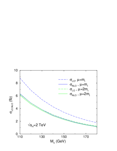
Fig. 4 shows both the LO and the NLO total cross section for $p\bar{p}\rightarrow t\bar{t}h$ at $\sqrt{s_{H}}\!=\!2$ TeV, for two values of the renormalization scale $\mu\!=\!m_{t}$ and $\mu\!=\!2m_{t}$. Over the entire range of $M_{h}$ accessible at the Tevatron, the NLO corrections decrease the rate. For example, for $M_{h}\!=\!120$ GeV and $\mu\!=\!m_{t}$ the NLO total cross section is reduced to $4.86\pm 0.03~{}fb$ from the lowest order prediction of $6.868\pm 0.002~{}fb$. The reduction is much less dramatic at $\mu\!=\!2m_{t}$, as can be seen from both Fig. 3 and Fig. 4. The complete NLO result includes the lowest order result and the contribution of the two terms given in Eq. (6). The error we quote on our values is the statistical error on the numerical integration involved in evaluating the total cross section.

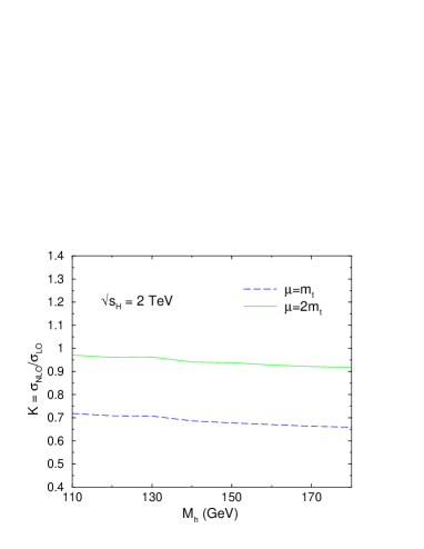
The corresponding K-factor, i.e. the ratio of the NLO cross section to the LO one

$$K=\frac{\sigma_{NLO}}{\sigma_{LO}}$$ (10)

is shown in Fig. 5. Given the strong scale dependence of the LO cross section, the K-factor also shows a significant $\mu$-dependence, while it is almost constant with $M_{h}$. For scales $\mu$ between $\mu\!=\!m_{t}$ and $\mu\!=\!2m_{t}$, the K-factor varies roughly between $K\!=\!0.70$ and $K\!=\!0.95$. The reduction of the NLO cross section with respect to the Born cross section is due to fact that at $\sqrt{s_{H}}\!=\!2$ TeV the $t\bar{t}h$ final state is produced in the threshold region. In this region the gluon exchange between the final state quarks gives origin to Coulomb singularities that contribute to the cross section with terms of order $\alpha_{s}/\beta$, where $\beta$ is the velocity of the top/antitop quark in the $t\bar{t}$ CM frame. Since the $t\bar{t}h$ final state is in a color octet configuration, these corrections are negative and therefore decreases the Born cross section, causing the K-factor to be smaller than unity. The same effect was observed in the NLO cross section for $e^{+}e^{-}\rightarrow t\bar{t}h$ [18]. In that case, however, the $t\bar{t}h$ final state is in a color singlet configuration and the threshold corrections are positive.

FIG. 4.: $\sigma_{NLO}$ and $\sigma_{LO}$ for $p{\overline{p}}\rightarrow t{\overline{t}}h$ as functions of $M_{h}$, at $\sqrt{s_{H}}\!=\!2$ TeV, for $\mu\!=m_{t}$ and $\mu\!=\!2m_{t}$.

FIG. 5.: K factor for $p{\overline{p}}\rightarrow t{\overline{t}}h$ as a function of $M_{h}$, at $\sqrt{s_{H}}\!=\!2$ TeV, for $\mu\!=m_{t}$ and $\mu\!=\!2m_{t}$ .

6. The next-to-leading order QCD corrections to the Standard Model process $p{\overline{p}}\rightarrow t{\overline{t}}h$, at $\sqrt{s_{H}}\!=\!2$ TeV, reduce the cross section by a factor of $0.7-0.95$ for renormalization and factorization scales $m_{t}\!<\!\mu\!<\!2m_{t}$. The NLO result shows a drastically reduced scale dependence as compared to the Born result and leads to increased confidence in predictions based on these results.

REFERENCES

- [1] T. Junk, Combined LEP Higgs Searches, Talk presented at the LEP Fest 2000, CERN, Oct. 2000.
- [2] A. Read, Report of the Higgs Working Group to LEPC (2000).
- [3] LEPEWWG/2001-01, May 2001.
- [4] S. Heinemeyer, W. Hollik and G. Weiglein, Eur. Phys. J. C 9, 343 (1999) [hep-ph/9812472].
- [5] M. Carena et al., “Report of the Tevatron Higgs working group”, hep-ph/0010338.
- [6] J. Goldstein, C. S. Hill, J. Incandela, S. Parke, D. Rainwater and D. Stuart, Phys. Rev. Lett. 86, 1694 (2001) [hep-ph/0006311].
- [7] J. Incandela, talk presented at the Workshop on the Future of Higgs Physics, Fermilab, May 3-5 2001.
- [8] L. Reina, S. Dawson, and D. Wackeroth, FSU-HEP-2001-0602, BNL-HET-01/19, UR-1639.
- [9] W. Beenakker, S. Dittmaier, M. Krämer, B. Plümper, M. Spira, and P. Zerwas, DESY 2001-077, Edinburgh 2001/08, PSI-PR-01-10.
- [10] S. Dawson and L. Reina, Phys. Rev. D 57, 5851 (1998) [hep-ph/9712400].
- [11] S. Dawson, L. Orr, L. Reina, and D. Wackeroth, work in progress.
- [12] J. A. M. Vermaseren, math-ph/0010025.
- [13] G. J. van Oldenborgh and J. A. Vermaseren, Z. Phys. C 46, 425 (1990).
- [14] Z. Bern, L. Dixon and D. A. Kosower, Phys. Lett. B 302, 299 (1993) [Erratum-ibid. B 318, 649 (1993)] [hep-ph/9212308]; Nucl. Phys. B 412, 751 (1994) [hep-ph/9306240].
- [15] J. Collins, F. Wilczek and A. Zee, Phys. Rev. D 18, 242 (1978); W. J. Marciano, Phys. Rev. D 29, 580 (1984) [Erratum-ibid. D 31, 213 (1984)].
- [16] B. W. Harris and J. F. Owens, hep-ph/0102128; U. Baur, S. Keller and D. Wackeroth, Phys. Rev. D 59, 013002 (1999) [hep-ph/9807417].
- [17] H. L. Lai et al., Phys. Rev. D 55, 1280 (1997) [hep-ph/9606399].
- [18] S. Dittmaier, M. Kramer, Y. Liao, M. Spira and P. M. Zerwas, Phys. Lett. B 441, 383 (1998) [hep-ph/9808433].