Quark correlations and gluon propagators in elastic vector meson production

Abstract

We study the behavior of the differential cross section for vector meson photoproduction at large momentum transfer in the two–gluon exchange model. We focus on the treatment of two–quark correlation function in the proton and on gluon propagators with a dynamically generated mass. We find that only the large $t$ region is sensitive to the particular details of these inputs.

1 INTRODUCTION

The exchange of two–gluons is the simplest realization of the pomeron in terms of the QCD degrees of freedom [1]. It was recently shown that the two–gluon exchange model can account for experimental data for the differential cross section of $\rho$ and $\phi$ photoproduction up to a momentum transfer of $-t\lesssim 6$ GeV² and $-t\lesssim 3$ GeV² respectively [2, 3], which is the largest momentum range available so far. One of the essential issues in getting such a good agreement was the role of quark correlations, i.e., diagrams where each gluon couples to a different quark in the proton.

As new data will become available from JLab for a wider range of $t$ it is important to study the predictions of the two–gluon exchange model in that region. In particular, our goal is to test the stability of these predictions against changes in the inputs of the model. We will focus on the study of the treatment of quark correlations in the proton and on the choice of the (non–perturbative) gluon propagator.

2 TWO–QUARK CORRELATION FUNCTION

It was argued that contributions from the diagram of Figure 1b, not included in the pomeron picture, are negligible as compared to the ones where both gluons couple to the same quark [4], Figure 1a. While this is true at low $t$, as $t$ increases both contributions become comparable and eventually the one of Figure 1b dominates [2].

At high energies the Dirac structure of the two–gluon coupling in Figure 1a is simply vector–like. Its contribution is proportional to the isoscalar Dirac form factor of the nucleon $F_{1}(-t)$, which is usually taken from fits to the experimental data. The diagram of Figure 1b is governed by a two–quark correlation function which, in the eikonal approximation [5], can be written as:

$$G_{2}(\vec{k}_{a},\vec{k}_{b})=\int\Pi_{i}dx_{i}d\vec{r}_{i}\delta(\sum_{i}x_{i}\vec{r}_{i})\delta(\sum_{i}x_{i}-1)|\Psi(x_{i},\vec{r}_{i})|^{2}e^{i(\vec{k}_{a}\cdot\vec{r}_{j}+\vec{k}_{b}\cdot\vec{r}_{k})}\;,$$ (1)

where $\vec{k}_{a}$, $\vec{k}_{b}$ are the (transverse) momenta flowing through each gluon ($(\vec{k}_{a}+\vec{k}_{b})^{2}=-t$) and $\Psi$ is the nucleon wave function which depend on the longitudinal momentum $x_{i}$ and the coordinates $\vec{r}_{i}$ in the transverse space. The evaluation of $G_{2}$ requires the explicit knowledge of the nucleon wave function. Nonetheless, this requirement is usually circumvented by making the approximation [6]:

$$G_{2}(\vec{k}_{a},\vec{k}_{b})=F_{1}(\vec{k}_{a}^{2}+\vec{k}_{b}^{2}-\vec{k}_{a}\cdot\vec{k}_{b}).$$ (2)

However, the expression above is strictly valid only when $x_{i}=1/3$. A more accurate approach that accounts for the smearing in the longitudinal momentum of the quarks obviously involves the explicit calculation of $G_{2}$ with a definite choice for the nucleon wave function. We have taken a simplified version of the wave function proposed in Ref. [7] and extensively used to evaluate (soft) contributions to a number of observables [8]. In momentum space it can be written as:

$$\Psi(x_{i},\vec{k}_{i})=N_{\Psi}\phi_{{\mbox{\small}AS}}\frac{1}{x_{1}x_{2}x_{3}}\exp[-a_{N}^{2}\sum_{i}\frac{\vec{k}_{i}^{2}}{x_{i}}]$$ (3)

where $N_{\Psi}$ is a normalization constant, $\phi_{{\mbox{\small}AS}}=120x_{1}x_{2}x_{3}$ is the asymptotic distribution amplitude for the nucleon and $\vec{k}_{i}$ refers to transverse momentum. We have fitted the free parameter $a_{N}$ to get a reasonable description of the isoscalar Dirac form factor of the nucleon. We get $a_{N}=1.25$ GeV^-1, which gives and averaged transverse momentum $\langle\vec{k}_{i}^{2}\rangle^{1/2}=0.325$ GeV.

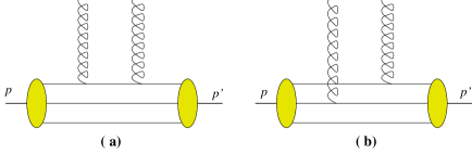
Figure 1: Coupling of the gluons to the valence quarks of the proton.

3 GLUON PROPAGATORS

Another important component in the two–gluon exchange model is the choice of the gluon propagator. In order to get an infrared safe behavior one has to deal with dressed propagators which are finite at the origin. From the physical viewpoint this prevents the gluon from propagating over very large distances. In order to match the successful description of cross sections provided by the pomeron the two–gluon exchange $qq\rightarrow qq$ amplitude is normalized at $t=0$ to the pomeron exchange amplitude, i.e.

$$\int_{0}^{\infty}dl^{2}[\alpha_{n}D(l^{2})]^{2}=\frac{9}{4\pi}\beta_{0}^{2}\;,$$ (4)

where $\beta_{0}=2$ GeV^-1 is the pomeron–quark coupling constant and $\alpha_{n}$ is an effective (frozen) value for the strong coupling constant which takes into account that we also deal with the non–perturbative domain.

It is customary to choose a Gaussian form for the gluon propagator:

$$\alpha_{n}D(l^{2})=\frac{3\beta_{0}}{\sqrt{2\pi}\lambda_{0}}\exp[-l^{2}/\lambda_{0}^{2}]\;,$$ (5)

where the parameter $\lambda_{0}^{2}=2.7$ GeV² is fixed to reproduce the total cross section for $\rho$ electroproduction [9].

A Gaussian propagator provides a reasonable agreement with a wide variety of experimental data [9]. However, it poses a conceptual problem since it does not have the right asymptotic behavior. A perturbative tail could be added by hand to Eq. (5), but it can be shown that the (Gaussian) non–perturbative part dominates the contribution to the differential cross section even at large $t$. An alternative path is to allow the gluon to have an effective mass which renders the perturbative propagator finite at the origin and has the right asymptotic behavior, provided that this mass vanishes at large momentum. Cornwall [10] derived an expression for a massive gluon propagator:

$$\alpha_{n}D(l^{2})=\frac{4\pi}{9}\frac{1}{[l^{2}+m^{2}(l^{2})]\log{[\frac{l^{2}+4m^{2}(l^{2})}{\Lambda^{2}}]}}$$ (6)

with a dynamically generated mass $m(l^{2})$ which has a logarithmic fall–off with the momentum. In order to set a common ground to compare with other approaches we have imposed the normalization condition (4) on this propagator and then we find $m(0)=396$ MeV for $\Lambda=300$ MeV. This value for $m(0)$ is within the range of the estimates of Cornwall ($m(0)=500\pm 200$ MeV) [10].

 

Figure 2: Differential cross section for $\phi$ photoproduction in the two–gluon exchange model (see text for explanation).

4 RESULTS

In Figure 2 we summarize our results for the differential cross section for $\phi$ photoproduction. The solid line represents the calculation with a Gaussian propagator and the assumption (2) for the two–quark correlation function. Results in Ref. [2] where obtained under these assumptions. If we explicitly calculate the function $G_{2}$ with the wave function (3) then we get the results represented by the dashed line in Figure 2. By comparing the two curves we can see that the specific way in which two–quark correlations are calculated has some effects only at large momentum transfer: at low and moderate $t$ it is the diagram of figure 1a, i.e. the isoscalar Dirac form factor, that dominates. Dashed–dotted line is obtained with $G_{2}$ evaluated with the nucleon wave function and the massive propagator for the gluon, Eq. (6). By comparing with the dashed line it is clear that the use of a massive propagator instead of the Gaussian one produces a further depletion in the differential cross section at large $t$. It also decreases slightly the slope at small $t$.

The same pattern of differences shown in Figure 2 is obtained for $\rho$ production. However, in that case, those differences are softened by quark–exchange contributions, which have to be incorporated before comparing with data [11].

It is worthwhile emphasizing that preliminary data from the CLAS Collaboration at JLab for $\phi$ photoproduction at $E_{\gamma}=4.5$ GeV supports the depletion obtained with the massive gluon propagator and the explicit calculation of $G_{2}$ (dashed–dotted line in Figure 2). Moreover, the use of a massive propagator is also essential in getting a definite asymptotic behavior for $d\sigma/dt$ at attainable values of $t$. We will address these issues in more detail in [11].

References

- [1] A. Donnachie and P.V. Landshoff, Nucl. Phys. B 311 (1989) 509.
- [2] J.-M. Laget, Phys. Lett. B 489 (2000) 313.
- [3] E. Anciant et al., Phys. Rev. Lett. 85 (2000) 4682.
- [4] P.V. Landshoff and O. Nachtmann, Z. Phys. C 35 (1987) 405.
- [5] J.F. Gunion and D.E. Soper, Phys. Rev. D 15 (1977) 2617.
- [6] J.R. Cudell and B.U. Nguyen, Nucl. Phys. B 420 (1994) 669.
- [7] J. Bolz and P. Kroll, Z. Phys. A 356 (1996) 327.
- [8] M. Diehl, Th. Feldmann, R. Jakob and P. Kroll, Eur. Phys. J. C 8 (1999) 409.
- [9] J.-M. Laget and R. Mendez-Galain, Nucl. Phys. A 581 (1995) 397.
- [10] J.M. Cornwall, Phys. Rev. D 26 (1982) 1453.
- [11] F. Cano and J.-M. Laget, in preparation.