Coulomb Gauge QCD, Confinement, and the Constituent Representation

Abstract

Quark confinement and the genesis of the constituent quark model are examined in nonperturbative QCD in Coulomb gauge. We employ a self-consistent method to construct a quasiparticle basis and to determine the quasiparticle interaction. The results agree remarkably well with lattice computations. They also illustrate the mechanism by which confinement and constituent quarks emerge, provide support for the Gribov-Zwanziger confinement scenario, clarify several perplexing issues in the constituent quark model, and permit the construction of an improved model of low energy QCD.

I Introduction

Two of the key issues facing QCD at low energy are a quantitative description of confinement and an understanding of the origins of the constituent quark model. In this paper we demonstrate how both issues may be resolved through a nonperturbative analysis of QCD in Coulomb gauge. This demonstration makes the physical origin of both effects clear, resolves several longstanding inconsistencies in the constituent quark model, significantly extends the quark model, and establishes a – perhaps surprising – relationship between confinement and the constituent quark model.

Although lattice gauge computations are capable of answering many questions in strong QCD, it is clear that the development of reliable analytical continuum tools are a necessity for advancing the field[1]. Continuum methods allow one to understand how QCD works from first principles, permit the development of intuition for phenomenological model building, and address computationally challenging phenomena such as QCD at finite density, extrapolation to low quark masses, or the treatment of large hadronic systems. A variety of such continuum tools exist: chiral perturbation theory, effective heavy quark and low energy hadronic field theories, 4-dimensional Dyson-Schwinger methods, fixed gauge Hamiltonian QCD approaches, and QCD sum rule methods. In this paper we focus on Hamiltonian QCD in Coulomb gauge.

Much progress has been made in understanding Coulomb gauge QCD since the seminal work of Schwinger[2], Khriplovich[3], and Christ and Lee[4]. In particular, the problem of the Gribov ambiguity[5] has been studied and a resolution has been suggested[6]. The ambiguity arises because of residual gauge freedom after the canonical Coulomb gauge fixing condition, $\nabla\cdot{\bf A}=0$ is imposed in a nonabelian theory. In Ref. [5] Gribov noted that the multiple-gauge copy ambiguity may be resolved by insisting that the Faddeev-Popov operator (to be defined later) is positive. With the aid of a simple model, he then showed that this constraint implies the existence of a novel form for the gluon propagator and an enhancement in the Faddeev-Popov propagator at low momenta. Furthermore, these imply that an enhancement exists in the instantaneous Coulomb potential, thereby providing a plausible mechanism for confinement. In a series of recent papers [6, 7], Zwanziger has brought the Gribov Coulomb gauge confinement scenario onto firm theoretical ground and has demonstrated that a complete definition of the Coulomb gauge may be achieved by restricting the gauge fields to the ‘fundamental modular region’ – defined as the set of gauge fields which form the absolute minima of a suitable functional. Furthermore, the constraint to the fundamental modular region may be imposed by introducing a horizon term through a Lagrange multiplier in the Hamiltonian.

A key feature of Coulomb gauge is that the elimination of nondynamical degrees of freedom creates an instantaneous interaction. The QED analogue of this is the Coulomb potential; however, the nonabelian nature of QCD causes this instantaneous interaction to depend on the gauge field, making it intrinsically nonperturbative for large fields. The restriction of the transverse gluon field to the fundamental modular region formally makes the Coulomb potential well defined. It also implies that the Faddeev-Popov (FP) operator which enters in the Coulomb potential is positive definite [6, 7]. A consequence of this is that one may employ the variational principle to build nonperturbative models of the QCD ground state. This is a crucial step with many phenomenological repercussions in the methodology we will be advocating. As we shall demonstrate, the Fock space which is built on our variational vacuum consists of quasiparticles – constituent quarks and gluons. These degrees of freedom obey dispersion relations with infrared divergences due to the long-range instantaneous Coulomb interaction of the bare partons with the mean field vacuum. This interaction makes colored objects infinitely heavy thus effectively removing them from the physical spectrum. However, color neutral states remain physical because the infrared singularities responsible for the large self-energies are canceled by infrared divergences responsible for the long-range forces between the constituents.

Constructing a quasiparticle basis is a nontrivial step which requires a nonperturbative treatment of QCD and, more directly, the QCD vacuum. We will show that it is possible to construct such a basis in a self-consistent manner by coupling a specific variational ansatz for the vacuum with the instantaneous interaction between color charges. The end results are explicit expressions for the Wilson confinement interaction, the spectrum of the quasiparticles, and the structure of the QCD vacuum. The resulting Fock space and effective Hamiltonian provide an ideal starting point for the examination of the bound state problem in QCD and provide a direct link between QCD and the phenomenological constituent quark model.

A simplified version of this program has been investigated by the authors and others before [8, 9, 10, 11, 12, 13, 14, 15, 16]. In several of these studies the nonabelian Coulomb interaction was replaced by an effective potential between color charges, leading to a relatively simple many-body Hamiltonian with two-body interactions between constituents. The phenomenology of this approach has proven quite successful. In Ref.[13] we have extended this simple approximation and treated the Coulomb kernel in a self-consistent way by considering the effect of resummation of a class of ladder diagrams. These diagrams originate from dressing the bare $\alpha_{S}/|{\bf x}-{\bf y}|$ Coulomb potential with transverse gluons. As one may expect from the discussion above, the effect of summing these diagrams is an enhancement of the Coulomb potential at large distances. Self-consistency appears in the problem because the strength of this enhancement is determined by the spectral properties the transverse gluons in the quasiparticle vacuum.

In this paper we build on these findings by constructing a fully self-consistent set of equations which describe the gluon dispersion relation, the effective instantaneous interaction, and the structure of the quasiparticle vacuum. A detailed derivation is given in Sec. II. This section also contains a brief review of the QCD Hamiltonian in Coulomb gauge and a discussion of the Gribov ambiguity. We discuss the renormalization procedure and show how the various counterterms in the regularized Coulomb gauge Hamiltonian may be constrained by physical observables. The last portion of Sec. II describes the variational vacuum employed in our method. Section III presents the solution to the coupled equations. We first discuss the details of the renormalization procedure and present an approximate analytical solution which demonstrates many of the features which emerge. This is followed by a full numerical solution and a discussion of the effects of higher order terms. A comparison of these results to lattice data is presented in Sec. IV. Section V discusses the implications of our results for the constituent quark model and phenomenology in general. This includes clarifying several open issues in the CQM and extending the CQM. A comparison to similar approaches and our conclusions are presented in Sec. VI.

II Quasiparticle Fock Space for Coulomb Gauge QCD and Confinement

One of the advantages of Coulomb gauge is that all degrees of freedom are physical. This makes the QCD Hamiltonian close in spirit to quantum mechanical models of QCD, for example the constituent quark model. The intuition gained from several decades of quark model calculations may then be applied to the analysis of a complex and nonlinear quantum field theory. Additional advantages of Coulomb gauge are that Gauss’s law is built into the Hamiltonian, the norm is positive definite, and no additional constraints need be imposed on Fock space. Furthermore, retardation effects are minimized for heavy quarks; thus this is a natural framework for studying nonrelativistic bound states, and in particular for identifying the physical mechanisms which drive relativistic corrections, e.g. the spin splittings in heavy quarkonia. Since chiral symmetry is dynamically broken this framework is also of relevance for light flavors once the constituent quarks are identified with the quasiparticle excitations.

The confinement phenomenon in QCD has two complementary aspects: (1) there is a long range attractive potential between colored sources; (2) the gluons which mediate this force are absent from the spectrum of physical states. Thus the mechanism for confinement is not particularly transparent [6] in covariant gauges. In Coulomb gauge, in contrast, these two aspects can comfortably co-exist: the long range force is represented by the instantaneous Coulomb interaction and is enhanced as ${\bf q}^{2}\to 0$, while the physical (transverse) gluon propagator is suppressed – reflecting the absence of colored states in the physical spectrum.

A Coulomb Gauge Hamiltonian

Since the Hamiltonian in Coulomb gauge may look unfamiliar to many readers we briefly illustrate the derivation of the classical Hamiltonian here.

The chromoelectric field is given by

$${\bf E}^{a}=-\dot{\bf A}^{a}-{\mbox{\boldmath$\nabla$}}A^{0a}+gf^{abc}A^{0b}{\bf A}^{c},$$ (1)

and satisfies Gauss’s law,

$${\mbox{\boldmath$\nabla$}}\cdot{\bf E}^{a}+gf^{abc}{\bf A}^{b}\cdot{\bf E}^{c}=g\rho^{a}_{q}.$$ (2)

Here $\rho^{a}_{q}=\psi^{{\dagger}}(\lambda^{a}/2)\psi$ is the quark color charge density. These equations are simplified by introducing the covariant derivative in the adjoint representation,

$${\bf D}^{ab}=\delta^{ab}{\mbox{\boldmath$\nabla$}}+igT^{c}_{ab}{\bf A}^{c},$$ (3)

where $T^{c}$ are the adjoint representation generators, $T^{c}_{ab}=if^{cab}$. Thus Eq. (2) becomes

$${\bf D}^{ab}\cdot{\bf E}^{b}=g\rho_{q}^{a}.$$ (4)

If the electric field is split into transverse and longitudinal pieces, ${\bf E}\equiv{\bf E}_{tr}-\nabla\phi$ then Eq. (4) yields

$$-({\bf D}^{ab}\cdot{\mbox{\boldmath$\nabla$}})\phi=g\rho^{a},$$ (5)

where $\rho^{a}=\rho^{a}_{q}+\rho^{a}_{g}$ is the full color charge density, with $\rho^{a}_{g}=f^{abc}{\bf E}^{b}_{tr}\cdot{\bf A}^{c}$ being the color charge density of transverse gluons. The equation of motion for the longitudinal component of the electric field,

$${\mbox{\boldmath$\nabla$}}\cdot{\bf E}^{a}=-{\mbox{\boldmath$\nabla$}}\cdot{\bf D}^{ab}A^{0b}=-{\mbox{\boldmath$\nabla$}}^{2}\phi^{a},$$ (6)

leads to a constraint for the 0-th component of the vector potential which can be formally solved. This yields

$$A^{0b}={1\over{\mbox{\boldmath$\nabla$}}\cdot{\bf D}}(-{\mbox{\boldmath$\nabla$}}^{2}){1\over{\mbox{\boldmath$\nabla$}}\cdot{\bf D}}g\rho^{b},$$ (7)

and

$$\phi^{a}={g\over{{\mbox{\boldmath$\nabla$}}\cdot{\bf D}}}\rho^{a}.$$ (8)

Finally the time evolution of the vector potential is determined by the transverse chromoelectric field through

$${\mbox{\boldmath$\Pi$}}^{a}\equiv-{\bf E}_{tr}^{a}=\dot{\bf A}^{a}-g(1-{\mbox{\boldmath$\nabla$}}^{-2}{\mbox{\boldmath$\nabla$}}{\mbox{\boldmath$\nabla$}}\cdot)f^{abc}A^{0b}{\bf A}^{c}.$$ (9)

After canonical quantization, the transverse field ${\mbox{\boldmath$\Pi$}}^{a}$ becomes the momentum conjugate to the transverse vector potential, ${\bf A}^{a}$.

Passing from the Lagrangian to the Hamiltonian yields terms proportional to $({\mbox{\boldmath$\nabla$}}\phi)^{2}$ from the longitudinal components of the chromoelectric field in ${\bf E}^{2}$, terms proportional to $g\rho_{q}A^{0}$ from the quark gluon vertex, $g{\bar{\psi}}\gamma^{0}A^{0a}\lambda^{a}/2\psi$ and terms proportional to $g\Pi^{a}\cdot{\bf A}^{b}A^{0c}f^{abc}$ from the ${\bf E}_{tr}\cdot\dot{{\bf A}_{tr}}$ pieces of ${\bf E}^{2}$. Combining all these contributions and substituting the expression for $A^{0}$ from Eq. (7) results in the instantaneous nonabelian Coulomb interaction,

$$H_{C}={1\over 2}\int d^{3}xd^{3}y\thinspace\rho^{a}({\bf x})K_{ab}({\bf x},{\bf y};{\bf A})\rho^{b}({\bf y}),$$ (10)

where

$$K_{ab}({\bf x},{\bf y};{\bf A})\equiv\langle{\bf x},a|{g\over{{\mbox{\boldmath$\nabla$}}\cdot{\bf D}}}(-{\mbox{\boldmath$\nabla$}}^{2}){g\over{{\mbox{\boldmath$\nabla$}}\cdot{\bf D}}}|{\bf y},b\rangle,$$ (11)

and $\rho^{a}$ is the full color charge density as derived above,

$$\rho^{a}({\bf x})=\rho^{a}_{g}({\bf x})+\rho^{a}_{q}({\bf x})=f^{abc}{\bf A}^{b}({\bf x})\cdot{\bf\Pi}^{c}({\bf x})+\psi^{{\dagger}}({\bf x}){\lambda^{a}\over 2}\psi({\bf x}).$$ (12)

The transverse conjugate gluon momenta ${\mbox{\boldmath$\Pi$}}^{a}$ satisfy

$$\left[A^{a,i}({\bf x}),\Pi^{b,j}({\bf y})\right]=i\delta^{ab}\left(\delta^{ij}-{{\nabla^{i}\nabla^{j}}\over{\mathchoice{{\hbox{\boldmath$\displaystyle\nabla$}}}{{\hbox{\boldmath$\textstyle\nabla$}}}{{\hbox{\boldmath$\scriptstyle\nabla$}}}{{\hbox{\boldmath$\scriptscriptstyle\nabla$}}}^{2}}}\right)\delta({\bf x}-{\bf y})\equiv i\delta^{ab}\delta_{T}(\hat{\mbox{\boldmath$\nabla$}})_{ij}\delta({\bf x}-{\bf y}).$$ (13)

Following Lee [17], we use the notation $\langle{\bf x},a|\cdots|{\bf y},b\rangle$ to denote kernels of integral operators,

$$\langle{\bf x},a|{\bf D}|{\bf y},b\rangle=\left[\delta^{ab}{\mbox{\boldmath$\nabla$}}_{{\bf x}}+gf^{acb}{\bf A}^{c}({\bf x})\right]\delta^{3}({\bf x}-{\bf y}).$$ (14)

In the abelian limit ${\bf D}\to{\mbox{\boldmath$\nabla$}}$, $K\to-g^{2}\langle{\bf x},a|1/{\mbox{\boldmath$\nabla$}}^{2}|{\bf y},b\rangle=g^{2}\delta^{ab}/4\pi|{\bf x}-{\bf y}|$ and the QED Coulomb interaction is recovered.

A rigorous derivation of the nonabelian, quantum Coulomb gauge Hamiltonian was given by Schwinger[2] and Christ and Lee[4]. Zwanziger has shown how to derive the Coulomb gauge Hamiltonian with a lattice regularization[6]. The quantum Hamiltonian may be derived by transforming the canonical $A^{0}=0$ Hamiltonian to Coulomb gauge. The $A^{0}=0$ Hamiltonian corresponds to ‘Cartesian’ coordinates in a flat gauge manifold, the subsequent restriction to Coulomb gauge induces curvature in the gauge manifold and therefore introduces a nontrivial metric. Christ and Lee have shown that the measure associated with this metric is proportional to the Faddeev-Popov determinant

$${\cal J}={\rm det}(\nabla\cdot D).$$ (15)

Furthermore, the Hamiltonian contains factors of ${\cal J}$ which are analogous to the Laplace-Beltrami operator induced when one first quantizes in curvilinear coordinates. The Faddeev-Popov determinant may be removed from the measure by working with the modified Hamiltonian

$$H\to{\cal J}^{1/2}H{\cal J}^{-1/2},$$ (16)

which is hermitian with respect to $(\Phi|\Psi)=\int{\cal D{\bf A}}\Phi^{*}({\bf A})\Psi({\bf A})$. Thus the final form for the QCD Hamiltonian in Coulomb gauge is

$$H=H_{q}+H_{g}+H_{qg}+H_{C},$$ (17)

where

$$H_{q}=\int d{\bf x}\psi^{\dagger}\left(-i\mathchoice{{\hbox{\boldmath$\displaystyle\alpha$}}}{{\hbox{\boldmath$\textstyle\alpha$}}}{{\hbox{\boldmath$\scriptstyle\alpha$}}}{{\hbox{\boldmath$\scriptscriptstyle\alpha$}}}\cdot{\mbox{\boldmath$\nabla$}}+\beta m\right)\psi,$$ (18)

$$H_{g}={1\over 2}\int d{\bf x}\left({\cal J}^{-1/2}{\mbox{\boldmath$\Pi$}}{\cal J}\cdot{\mbox{\boldmath$\Pi$}}{\cal J}^{-1/2}+{\bf B}\cdot{\bf B}\right),$$ (19)

$$H_{qg}=-g\int d{\bf x}\psi^{\dagger}\mathchoice{{\hbox{\boldmath$\displaystyle\alpha$}}}{{\hbox{\boldmath$\textstyle\alpha$}}}{{\hbox{\boldmath$\scriptstyle\alpha$}}}{{\hbox{\boldmath$\scriptscriptstyle\alpha$}}}\cdot{\bf A}\psi,$$ (20)

and

$$H_{C}={1\over 2}\int d{\bf x}d{\bf y}{\cal J}^{-1/2}\rho^{a}(x){\cal J}^{1/2}K_{ab}({\bf x},{\bf y};{\bf A}){\cal J}^{1/2}\rho^{b}(y){\cal J}^{-1/2},$$ (21)

In order to compare with the covariant Feynman rules and the canonical path integral formalism, it is convenient to Weyl order the operators (we note that Weyl ordering is the operator ordering which corresponds to path integral quantization with midpoint discretization). This leads to the Schwinger-Christ-Lee terms, $V_{1}$ and $V_{2}$ [17]. Here we will keep the original ordering of Eqs. (17-21) so that no explicit $V_{1}$ and $V_{2}$ terms are present.

B The Gribov Ambiguity

As detailed by Zwanziger [18], not only is the Hamiltonian renormalizable in Coulomb gauge but the Gribov problem can also be resolved [6]. The essence of the Gribov problem is that the condition ${\mbox{\boldmath$\nabla$}}\cdot{\bf A}=0$ does not uniquely fix the gauge in non-Abelian gauge theories; in general there are many copies of gauge field configurations, all with the same divergence, which are related by gauge transformations. Alternatively, the canonical transformation to Coulomb gauge is not singular so long as ${\rm det}(\nabla\cdot D)\neq 0$. But Gribov has shown that large gauge configurations exist such that this condition does not hold. As the true physical configuration space of a gauge theory is the set of gauge potentials modulo local gauge transformations, one must select a single representative from each set of gauge-equivalent configurations. The resulting subset of independent field configurations is known as the fundamental modular region (FMR).

A convenient characterization of the FMR is given by the “minimal” Coulomb gauge, obtained by minimizing a suitably chosen functional over gauge orbits. This functional is defined as

$$F_{\bf A}[g]={\rm Tr}\int d^{3}x({\bf A}^{g})^{2}\;,$$ (22)

where $g({\bf x})$ is a gauge transformation and ${\bf A}^{g}=g{\bf A}g^{\dagger}-g{\mbox{\boldmath$\nabla$}}g^{\dagger}$. A simple calculation show that fields in the FMR are transverse. Alternatively, Zwanziger has demonstrated that Gribov copies may be removed by imposing the constraint $\langle G\rangle/{\cal V}=0$ (called the horizon condition) and argued that in the infinite volume limit imposing the horizon condition enables one to remove the direct restriction on the fields. Here $G$ is the ‘horizon term’ given by

$$G=\int d{\bf x}\,d{\bf y}\,{\bf D}^{ca}(x)\cdot\langle{\bf x}a|{-1\over{\mbox{\boldmath$\nabla$}}\cdot{\bf D}}|{\bf y}b\rangle\cdot{\bf D}^{bc}(y)+(N_{c}^{2}-1){\cal V}.$$ (23)

In this paper we follow a third approach. Because the Faddeev-Popov operator is positive semi-definite for fields in the FMR, we expand it in a power series over field variables and evaluate matrix elements by integrating over all fields. This is justified as long as the expectation value of the Faddeev-Popov operator does not change sign. We discuss under what conditions this procedure is consistent with the horizon condition in Sec. IV.B.

C Regularization and Renormalization

To properly define the Hamiltonian a cutoff must be introduced to regularize ultraviolet divergences. This can be done, for example, by point splitting products of fields in the Hamiltonian. A simpler regularization procedure, adopted here, is to smear the fields. The induced nonlocalities are removed as the cutoff is taken to infinity. Since in the numerical studies to follow we will be working with renormalized quantities only (which are cutoff independent), we will explicitly remove the regulator making details of the regularization irrelevant.

Counterterms need to be added to the canonical Hamiltonian to ensure that a cutoff independent spectrum is produced,

$$H\to H(\Lambda)\to H(\Lambda)+\delta H(\Lambda).$$ (24)

In this paper we concentrate on the pure glue sector with at most static quarks, and therefore we will ignore the part of the Hamiltonian involving momentum or spin of the quarks. In the gluon sector, the presence of the cutoff leads to a single relevant operator (an operator whose canonical dimension is less then four). Thus $\delta H(\Lambda)$ contains a term

$$\delta H(\Lambda)=\Lambda^{2}{{Z_{m}(\Lambda)}\over 2}\int d{\bf x}\left[{\bf A}^{a}({\bf x})^{2}\right]_{\Lambda}+\cdots$$ (25)

where $Z_{m}(\Lambda)$ is a dimensionless constant, and the notation $[\cdots]_{\Lambda}$ represents the effect of regularization. For all marginal dimension four operators present in the canonical Hamiltonian there will be corresponding operators in $\delta H(\Lambda)$ and the combination of the two leads to a Hamiltonian in which canonical terms are multiplied by $\Lambda$-dependent renormalization constants. For example,

$$\int d{\bf x}\left[{\mathchoice{{\hbox{\boldmath$\displaystyle\Pi$}}}{{\hbox{\boldmath$\textstyle\Pi$}}}{{\hbox{\boldmath$\scriptstyle\Pi$}}}{{\hbox{\boldmath$\scriptscriptstyle\Pi$}}}}^{a}({\bf x})^{2}\right]_{\Lambda}+\delta\int d{\bf x}\left[{\mathchoice{{\hbox{\boldmath$\displaystyle\Pi$}}}{{\hbox{\boldmath$\textstyle\Pi$}}}{{\hbox{\boldmath$\scriptstyle\Pi$}}}{{\hbox{\boldmath$\scriptscriptstyle\Pi$}}}}^{a}({\bf x})^{2}\right]_{\Lambda}\equiv Z_{\Pi}(\Lambda)\int d{\bf x}\left[{\mathchoice{{\hbox{\boldmath$\displaystyle\Pi$}}}{{\hbox{\boldmath$\textstyle\Pi$}}}{{\hbox{\boldmath$\scriptstyle\Pi$}}}{{\hbox{\boldmath$\scriptscriptstyle\Pi$}}}}^{a}({\bf x})^{2}\right]_{\Lambda}.$$ (26)

The full regularized Hamiltonian with counterterms is then given by

$$H = {{Z_{\Pi}(\Lambda)}\over 2}\int d{\bf x}\left[\mathchoice{{\hbox{\boldmath$\displaystyle\Pi$}}}{{\hbox{\boldmath$\textstyle\Pi$}}}{{\hbox{\boldmath$\scriptstyle\Pi$}}}{{\hbox{\boldmath$\scriptscriptstyle\Pi$}}}^{a}({\bf x})^{2}\right]_{\Lambda}+{{Z_{A}(\Lambda)}\over 2}\int d{\bf x}\left[{\bf B}^{a}({\bf x})^{2}\right]_{\Lambda}+\Lambda^{2}{{Z_{m}(\Lambda)}\over 2}\int\left[{\bf A}^{a}({\bf x})^{2}\right]_{\Lambda}$$ (28)

$$+{{Z_{K}(\Lambda)}\over 2}\int d{\bf x}d{\bf y}\left[\rho^{a}({\bf x})K_{ab}({\bf x},{\bf y};{\bf A})\rho^{b}({\bf y})\right]_{\Lambda}+\ldots$$

The ellipsis stands for higher order terms induced by expanding the modified conjugate momenta ${\cal J}^{-1/2}{\mbox{\boldmath$\Pi$}}{\cal J}^{1/2}$ in terms of gauge potentials. The effect of these terms will be discussed in Sec. III.F.

At this stage we should in principle allow for every composite operator of dimension $d$ appearing in the Hamiltonian to be multiplied by a renormalization factor $Z(\Lambda)\Lambda^{4-d}$ with $Z$ being dimensionless and also allow for the coupling constant to be $\Lambda$ dependent $g\to Z_{g}(\Lambda)g\equiv g(\Lambda)$. For example, as discussed earlier, if the fields are in the FMR the Coulomb kernel may be expanded in a power series in $g{\bf A}$, and the order $n$ contribution would be proportional to

$$Z_{n}(\Lambda)\left[{{ig(\Lambda)}\over{{\mbox{\boldmath$\nabla$}}^{2}}}{\bf A}^{c}T^{c}\cdot{\mbox{\boldmath$\nabla$}}\right]^{n}_{\Lambda}.$$ (29)

Here $Z_{n}(\Lambda)$ is the $n$-th order triple gluon vertex (two Coulomb and one transverse) renormalization constant and $g(\Lambda)$ is the renormalized coupling. As we will show in Sec. III.F such vertices are UV finite which implies $Z_{i}(\Lambda)=1$. The contribution from the Coulomb kernel to the Hamiltonian can therefore be written in terms of only two renormalization constants $Z_{K}(\Lambda)$ and $Z_{m}(\Lambda)$ (and implicitly $g(\Lambda)$) as in Eq. (28).

As mentioned above, the $\Lambda$ dependence of all renormalization constants has to be adjusted in such a way that $H$ leads to a $\Lambda$-independent spectrum. This implies that the renormalization group equations may be determined nonperturbatively from the spectrum of $H$. Furthermore in order for this Hamiltonian to be consistent with QCD (in the chiral limit) all renormalization constants $Z_{i}(\Lambda)$ cannot depend on $\Lambda$ in an arbitrary way, but instead should depend on the scale through the coupling $g(\Lambda)$. The renormalization group equations will be discussed in Sec. III.C.

D Vacuum Structure

The eigenstates of the Hamiltonian can, in principle, be expanded in an arbitrarily chosen complete basis which spans Fock space. One choice would be to use the perturbative basis which diagonalizes the free Hamiltonian $H(g=0)$. However, one expects the description of any hadronic bound state would be very complicated in this basis. Alternatively, the phenomenologically successful constituent quark model indicates that hadronic wavefunctions may saturate quickly with only a few Fock space states provided these states are constructed from constituent (quasiparticle) quarks. This strongly suggests that a basis which incorporates the effects of spontaneous chiral symmetry breaking would be more efficient for describing hadrons and their interactions.

We expect a similar scenario to apply to the gluon sector. In a given hadronic state there is a large probability of finding a component with a large number of bare, massless transverse gluons, but the expansion of a hadronic state may be significantly simplified in a transformed Fock space which is constructed from quasiparticle (massive constituent) gluons. We follow this intuition by constructing a vacuum upon which the quasiparticle basis is built with a functional Gaussian ansatz[19],

$$\Psi_{0}[{\bf A}]=\langle{\bf A}|\omega\rangle=\exp\left[-{1\over 2}\int{{d{\bf k}}\over{(2\pi)^{3}}}{\bf A}^{a}({\bf k})\,\omega(k){\bf A}^{a}(-{\bf k})\right].$$ (30)

It may be shown[20] that this ansatz sums all diagrams with nonoverlapping divergences. Note that the perturbative vacuum is obtained when $\omega=|{\bf k}|$. The trial function is obtained by minimizing the vacuum energy density

$${{\delta}\over{\delta\omega}}\langle\omega|H|\omega\rangle=0.$$ (31)

The vacuum state obtained from this procedure is denoted $|\omega\rangle$. We refer to $\omega$ as the gap function since it is also responsible for lifting the single particle gluon energy beyond its perturbative value (see Fig. 5 below).

This procedure is formally equivalent to the Hartree-Fock-Bogoliubov approximation, therefore one may also determine $\omega$ with a suitably chosen canonical transformation. Perturbative gluon creation and annihilation operators are introduced in the standard way,

$${\bf A}^{c}({\bf x}) = \int{{d{\bf k}}\over{(2\pi)^{3}}}{1\over{\sqrt{2k}}}\left[\mathchoice{{\hbox{\boldmath$\displaystyle\epsilon$}}}{{\hbox{\boldmath$\textstyle\epsilon$}}}{{\hbox{\boldmath$\scriptstyle\epsilon$}}}{{\hbox{\boldmath$\scriptscriptstyle\epsilon$}}}({\bf k},\lambda)a({\bf k},\lambda,c)+\mathchoice{{\hbox{\boldmath$\displaystyle\epsilon$}}}{{\hbox{\boldmath$\textstyle\epsilon$}}}{{\hbox{\boldmath$\scriptstyle\epsilon$}}}{{\hbox{\boldmath$\scriptscriptstyle\epsilon$}}}^{*}({\bf k},\lambda)a^{{\dagger}}(-{\bf k},\lambda,c)\right]e^{i{\bf k}\cdot{\bf x}},$$ (32)

$$\mathchoice{{\hbox{\boldmath$\displaystyle\Pi$}}}{{\hbox{\boldmath$\textstyle\Pi$}}}{{\hbox{\boldmath$\scriptstyle\Pi$}}}{{\hbox{\boldmath$\scriptscriptstyle\Pi$}}}^{c}({\bf x}) = -i\int{{d{\bf k}}\over{(2\pi)^{3}}}\sqrt{k\over 2}\left[\mathchoice{{\hbox{\boldmath$\displaystyle\epsilon$}}}{{\hbox{\boldmath$\textstyle\epsilon$}}}{{\hbox{\boldmath$\scriptstyle\epsilon$}}}{{\hbox{\boldmath$\scriptscriptstyle\epsilon$}}}({\bf k},\lambda)a({\bf k},\lambda,c)-\mathchoice{{\hbox{\boldmath$\displaystyle\epsilon$}}}{{\hbox{\boldmath$\textstyle\epsilon$}}}{{\hbox{\boldmath$\scriptstyle\epsilon$}}}{{\hbox{\boldmath$\scriptscriptstyle\epsilon$}}}^{*}({\bf k},\lambda)a^{{\dagger}}(-{\bf k},\lambda,c)\right]e^{i{\bf k}\cdot{\bf x}},$$ (33)

with the perturbative vacuum satisfying, $a({\bf k},\lambda,c)|\omega(k)=k\rangle=0$. The canonical transformation is determined by requiring that the vacuum ansatz satisfies $\alpha({\bf k},\lambda,c)|\omega\rangle=0$, where the quasiparticle operators $\alpha,\alpha^{{\dagger}}$ are related to the fields by

$${\bf A}^{c}({\bf x}) = \int{{d{\bf k}}\over{(2\pi)^{3}}}{1\over{\sqrt{2\omega(k)}}}\left[\mathchoice{{\hbox{\boldmath$\displaystyle\epsilon$}}}{{\hbox{\boldmath$\textstyle\epsilon$}}}{{\hbox{\boldmath$\scriptstyle\epsilon$}}}{{\hbox{\boldmath$\scriptscriptstyle\epsilon$}}}({\bf k},\lambda)\alpha({\bf k},\lambda,c)+\mathchoice{{\hbox{\boldmath$\displaystyle\epsilon$}}}{{\hbox{\boldmath$\textstyle\epsilon$}}}{{\hbox{\boldmath$\scriptstyle\epsilon$}}}{{\hbox{\boldmath$\scriptscriptstyle\epsilon$}}}^{*}({\bf k},\lambda)\alpha^{{\dagger}}(-{\bf k},\lambda,c)\right]e^{i{\bf k}\cdot{\bf x}},$$ (34)

$$\mathchoice{{\hbox{\boldmath$\displaystyle\Pi$}}}{{\hbox{\boldmath$\textstyle\Pi$}}}{{\hbox{\boldmath$\scriptstyle\Pi$}}}{{\hbox{\boldmath$\scriptscriptstyle\Pi$}}}^{c}({\bf x}) = -i\int{{d{\bf k}}\over{(2\pi)^{3}}}\sqrt{{\omega(k)}\over 2}\left[\mathchoice{{\hbox{\boldmath$\displaystyle\epsilon$}}}{{\hbox{\boldmath$\textstyle\epsilon$}}}{{\hbox{\boldmath$\scriptstyle\epsilon$}}}{{\hbox{\boldmath$\scriptscriptstyle\epsilon$}}}({\bf k},\lambda)\alpha({\bf k},\lambda,c)-\mathchoice{{\hbox{\boldmath$\displaystyle\epsilon$}}}{{\hbox{\boldmath$\textstyle\epsilon$}}}{{\hbox{\boldmath$\scriptstyle\epsilon$}}}{{\hbox{\boldmath$\scriptscriptstyle\epsilon$}}}^{*}({\bf k},\lambda)\alpha^{{\dagger}}(-{\bf k},\lambda,c)\right]e^{i{\bf k}\cdot{\bf x}}.$$ (35)

The condition that emerges for $\omega(k)$ from Eq. (31) is identical to the condition that there are no $\alpha^{{\dagger}}\alpha^{{\dagger}}$ or $\alpha\alpha$ operators in the full Hamiltonian.

E Self-Consistent Gap Equations

The form of the QCD Hamiltonian in Coulomb gauge induces a crucial complication in the evaluation of the ground state energy density. This is because the interaction potential itself depends on the choice of the vacuum: the kernel $K$ (Eq. 11) depends on the vector fields which depend on the gap function (Eq. 32). Thus the gap function is actually determined by a set of coupled equations which describe the vacuum energy density and the interactions which are used to obtain this energy density. This subsection describes how these equations are obtained; the solution is presented in the next section.

The first step is the evaluation of the Coulomb kernel, Eq. (11). This is greatly simplified with the aid of the Swift equation[21]:

$$K_{ab}({\bf x},{\bf y};{\bf A})_{\Lambda},=g^{2}(\Lambda){d\over{dg(\Lambda)}}\langle{\bf x},a|{{g(\Lambda)}\over{{\mbox{\boldmath$\nabla$}}\cdot D}}|{\bf x},b\rangle.$$ (36)

The subscript $\Lambda$ refers to the regularization of fields operators in the Coulomb kernel. Thus one need only evaluate the Faddeev-Popov operator $g/\nabla\cdot{\bf D}$ to obtain the full instantaneous Coulomb kernel. This can be done by expanding the Faddeev-Popov operator in powers of $g{\bf A}$ and taking the appropriate contractions of the gluon field. The expansion is justified as long as the fields are restricted to the fundamental modular region. In the infinite volume limit, this restriction is not expected to affect field contractions[7] as long as the expectation value of the horizon term vanishes. Thus the following expressions may be used,

$$\langle\omega|\left[{\bf A}^{a}({\bf x}){\bf A}^{b}({\bf y})\right]_{\Lambda}|\omega\rangle = {\delta_{ab}\over 2}\int^{\Lambda}dk{{\delta_{T}(\hat{\bf k})}\over{\omega({\bf k};\Lambda)}}e^{i{\bf k}\cdot({\bf x}-{\bf y})},$$ (37)

$$\langle\omega|\left[\mathchoice{{\hbox{\boldmath$\displaystyle\Pi$}}}{{\hbox{\boldmath$\textstyle\Pi$}}}{{\hbox{\boldmath$\scriptstyle\Pi$}}}{{\hbox{\boldmath$\scriptscriptstyle\Pi$}}}^{a}({\bf x})\mathchoice{{\hbox{\boldmath$\displaystyle\Pi$}}}{{\hbox{\boldmath$\textstyle\Pi$}}}{{\hbox{\boldmath$\scriptstyle\Pi$}}}{{\hbox{\boldmath$\scriptscriptstyle\Pi$}}}^{b}({\bf y})\right]_{\Lambda}|\omega\rangle = {\delta_{ab}\over 2}\int^{\Lambda}dk\delta_{T}(\hat{\bf k})\omega(k;\Lambda)e^{i{\bf k}\cdot({\bf x}-{\bf y})},$$ (38)

$$\langle\omega|\left[{\bf A}^{a}({\bf x})\mathchoice{{\hbox{\boldmath$\displaystyle\Pi$}}}{{\hbox{\boldmath$\textstyle\Pi$}}}{{\hbox{\boldmath$\scriptstyle\Pi$}}}{{\hbox{\boldmath$\scriptscriptstyle\Pi$}}}^{b}({\bf y})\right]_{\Lambda}|\omega\rangle = -\langle\omega|\left[\mathchoice{{\hbox{\boldmath$\displaystyle\Pi$}}}{{\hbox{\boldmath$\textstyle\Pi$}}}{{\hbox{\boldmath$\scriptstyle\Pi$}}}{{\hbox{\boldmath$\scriptscriptstyle\Pi$}}}^{a}({\bf x}){\bf A}^{b}({\bf y})\right]_{\Lambda}|\omega\rangle=i{\delta_{ab}\over 2}\int^{\Lambda}dk\delta_{T}(\hat{\bf k})e^{i{\bf k}\cdot({\bf x}-{\bf y})}.$$ (39)

We have temporarily allowed for $\Lambda$-dependence in the gap function. This is discussed in more detail in Sec. III.A.

The expansion of the Faddeev-Popov operator is given by

$$\langle{\bf x}a|{{g(\Lambda)}\over{{\mbox{\boldmath$\nabla$}}\cdot{\bf D}}}|{\bf y},b\rangle_{\Lambda}=D^{(0)}({\bf x},{\bf y};\Lambda)\delta_{ab}+\sum_{c_{1},i_{1}}\int d{\bf z}_{1}D^{(1)c_{1}}_{i_{1}}({\bf x},{\bf y},{\bf z}_{1};\Lambda)_{ab}:A^{c_{1},i_{1}}({\bf z}_{1}):_{\Lambda}$$ (40)

$$+\ldots\sum_{c_{1}\cdots c_{n}}\sum_{i_{1}\cdots i_{n}}\int d{\bf z}_{1}\cdots d{\bf z}_{n}D^{(n)c_{1}\cdots c_{n}}_{i_{1}\cdots i_{n}}({\bf x},{\bf y},{\bf z}_{1},\cdots{\bf z}_{n};\Lambda)_{ab}:A^{c_{1},i_{1}}({\bf z}_{1})\cdots A^{c_{n},i_{n}}({\bf z}_{n}):_{\Lambda}+\ldots,$$ (41)

(42)

where $::$ stands for normal ordering with respect to $|\omega\rangle$ and $c_{n}$ and $i_{n}$ refer to color and spatial components of the gluon field respectively. Here $D^{(0)}$ stands for the expectation value (VEV) of the Faddeev-Popov operator in the ansatz vacuum,

$$D^{(0)}_{ab}({\bf x},{\bf y};\Lambda)=\langle\omega|\langle{\bf x}a|{{g(\Lambda)}\over{{\mbox{\boldmath$\nabla$}}\cdot{\bf D}}}|{\bf y},b\rangle|\omega\rangle_{\Lambda}$$ (43)

An operator expansion of the Coulomb kernel may be defined in a similar manner

$$K_{ab}({\bf x},{\bf y};{\bf A})=K^{(0)}({\bf x},{\bf y};\Lambda)\delta_{ab}+\sum_{c_{1},i_{1}}\int d{\bf z}_{1}K^{(1)c_{1}}_{i_{1}}({\bf x},{\bf y},{\bf z}_{1};\Lambda)_{ab}:A^{c_{1},i_{1}}({\bf z}_{1}):_{\Lambda}$$ (44)

$$+\ldots\sum_{c_{1}\cdots c_{n}}\sum_{i_{1}\cdots i_{n}}\int d{\bf z}_{1}\cdots d{\bf z}_{n}K^{(n)c_{1}\cdots c_{n}}_{i_{1}\cdots i_{n}}({\bf x},{\bf y},{\bf z}_{1},\cdots{\bf z}_{n};\Lambda)_{ab}:A^{c_{1},i_{1}}({\bf z}_{1})\cdots A^{c_{n},i_{n}}({\bf z}_{n}):_{\Lambda}+\ldots$$ (45)

(46)

The equation for the VEV of the FP operator is most easily expressed in terms of its Fourier transform which we write as

$$(2\pi)^{3}\delta({\bf P}){{d({\bf k};\Lambda)}\over{{\bf k}^{2}}}\delta_{ab}\equiv-\int d{\bf x}d{\bf y}D^{(0)}_{ab}({\bf x},{\bf y};\Lambda)e^{i{\bf k}\cdot({\bf x}-{\bf y})}e^{i{\bf P}\cdot{{{\bf x}+{\bf y}}\over 2}}.$$ (47)

The amplitudes $D^{(n)}$ which multiply a product of $n$ gluon fields can be written in terms of $D^{(0)}$ and a set of vertex functions, $\Gamma^{(n)}$. To do this we first define the Fourier transform of the $D^{(n)}$ via

$$(2\pi)^{3}\delta({\bf k}-\sum_{i=1}^{n}{\bf q}_{i}-{\bf l})d^{(n)c_{1}\cdots c_{n}}_{i_{1}\cdots,i_{n}}({\bf k},{\bf q}_{1},\cdots,{\bf q}_{n},{\bf l};\Lambda) \equiv-\int d{\bf x}d{\bf y}d{\bf z}_{1}\cdots d{\bf z}_{n}e^{-i{\bf k}\cdot{\bf x}+i{\bf l}\cdot{\bf y}+i\sum_{i=1}^{n}{\bf q}_{i}\cdot{\bf z}_{i}}$$ (49)

$$\times D^{(n)c_{1}\cdots c_{n}}_{i_{1}\cdots,i_{n}}({\bf x},{\bf z}_{1},\cdots,{\bf z}_{n},{\bf y};\Lambda)$$

Next we define the full transverse gluon-Coulomb vertex as $\Gamma^{c}_{i}({\bf k},{\bf q},{\bf p})$. The Dyson equation for the full vertex is illustrated in Fig. 1 and is given by

$$\Gamma^{c}_{i}({\bf k},{\bf q},{\bf k}-{\bf q};\Lambda)=Z_{1}(\Lambda)T^{c}k^{i}+\sum_{c_{1}}\sum_{i_{1}}\int^{\Lambda}{{d{\bf l}}\over{(2\pi)^{3}}}{1\over{2\omega(l;\Lambda)}}\left[\Gamma^{c_{1}}_{i_{1}}({\bf k},{\bf l},{\bf k}-{\bf l};\Lambda){{d({\bf k}-{\bf l};\Lambda)}\over{({\bf k}-{\bf l})^{2}}}\right.$$ (50)

$$\times\left.\Gamma^{c}_{i}({\bf k}-{\bf l},{\bf q},{\bf k}-{\bf l}-{\bf q};\Lambda){{d({\bf k}-{\bf l}-{\bf q};\Lambda)}\over{({\bf k}-{\bf l}-{\bf q})^{2}}}\Gamma^{c_{1}}_{i_{1}}({\bf k}-{\bf l}-{\bf q},{\bf l},{\bf k}-{\bf q};\Lambda)\right].$$ (51)

FIG. 1.: Dyson equation of the Coulomb-transverse gluon vertex. The thick line represents the full FP function $d({\bf k})$. The hatched circle represents the full vertex $\Gamma^{c}_{i}$. The gluon line is the gluonic quasiparticle. All external propagators are truncated.

In the planar approximation higher order vertex functions $\Gamma^{(n)}$ satisfy the following Dyson equation,

$$\Gamma^{(n);c_{1}\cdots c_{n}}_{i_{1}\cdots i_{n}}({\bf k},{\bf q}_{1},\cdots,{\bf q}_{n},{\bf k}-\sum_{i=1}^{n}{\bf q}_{i})=\tilde{\Gamma}^{(n);c_{1}\cdots c_{n}}_{i_{1}\cdots i_{n}}({\bf k},{\bf q}_{1},\cdots,{\bf q}_{n},{\bf k}-\sum_{i=1}^{n}{\bf q}_{i})$$ (52)

$$+\sum_{c_{0}}\sum_{i_{0}}\int{{d{\bf q}_{0}}\over{(2\pi)^{3}}}{1\over{2\omega(q_{0})}}\left[\Gamma^{c_{0}}_{i_{0}}({\bf k},{\bf q}_{0},{\bf k}-{\bf q}_{0}){{d({\bf k}-{\bf q}_{0})}\over{({\bf k}-{\bf q}_{0})^{2}}}\tilde{\Gamma}^{(n);c_{1}\cdots c_{n}}_{i_{1}\cdots i_{n}}({\bf k}-{\bf q}_{0},{\bf q}_{1}\cdots{\bf q}_{n},{\bf k}-{\bf q}_{0}-\sum_{i=1}^{n}{\bf q}_{i})\right.$$ (53)

$$\times\left.{{d({\bf k}-{\bf q}_{0}-\sum_{i=1}^{n}{\bf q}_{n})}\over{({\bf k}-{\bf q}_{0}-\sum_{i=1}^{n}{\bf q}_{n})^{2}}}\Gamma^{c_{0}}_{i_{0}}({\bf k}-{\bf q}_{0}-\sum_{i=1}^{n}{\bf q}_{n},{\bf q}_{0},{\bf k}-\sum_{i=1}^{n}{\bf q}_{n})\right],$$ (54)

where we have introduced the following quantity:

$$\tilde{\Gamma}^{(n);c_{1}\cdots c_{n}}_{i_{1}\cdots i_{n}}({\bf k},{\bf q}_{1},\cdots,{\bf q}_{n},{\bf k}-\sum_{i=1}^{n}{\bf q}_{i})\equiv\sum_{c_{0}}\sum_{i_{0}}\int{{d{\bf q}_{0}}\over{(2\pi)^{3}}}{1\over{2\omega(q_{0})}}\left[\Gamma^{c_{0}}_{i_{0}}({\bf k},{\bf q}_{0},{\bf k}-{\bf q}_{0}){{d({\bf k}-{\bf q}_{0})}\over{({\bf k}-{\bf q}_{0})^{2}}}\right.$$ (55)

$$\times\left.\Gamma^{c_{1}}_{i_{1}}({\bf k}-{\bf q}_{0},{\bf q}_{1},{\bf k}-{\bf q}_{0}-{\bf q}_{1}){{d({\bf k}-{\bf q}_{0}-{\bf q}_{1})}\over{({\bf k}-{\bf q}_{0}-{\bf q}_{1})^{2}}}\times\right.$$ (56)

$$\left.\cdots\times\Gamma^{c_{n}}_{i_{n}}({\bf k}-{\bf q}_{0}-\sum_{i=1}^{n-1}{\bf q}_{i},{\bf q}_{n},{\bf k}-{\bf q}_{0}-\sum_{i=1}^{n}{\bf q}_{i}){{d({\bf k}-{\bf q}_{0}-\sum_{i=1}^{n}{\bf q}_{n})}\over{({\bf k}-{\bf q}_{0}-\sum_{i=1}^{n}{\bf q}_{n})^{2}}}\right.$$ (57)

$$\times\left.\Gamma^{c_{0}}_{i_{0}}({\bf k}-{\bf q}_{0}-\sum_{i=1}^{n}{\bf q}_{n},{\bf q}_{0},{\bf k}-\sum_{i=1}^{n}{\bf q}_{n})\right].$$ (58)

(59)

FIG. 2.: Dyson equation for $\Gamma^{(2)}$. Symbols are as in Fig. 1.

The equation for $\Gamma^{(2)}$ is shown in Fig. 2.

Finally, we are able to write the coefficients of the operator product expansion of the Faddeev-Popov operator as

$$d^{(1)}_{c;i}({\bf k},{\bf q},{\bf k}-{\bf q})=d({\bf k})\Gamma^{c}_{i}({\bf k},{\bf q},{\bf k}-{\bf q})d({\bf q})$$ (60)

and

$$d^{(2)}_{c_{1},c_{2};i_{1},i_{2}}({\bf k},{\bf q}_{1},{\bf q}_{2},{\bf k}-{\bf q}_{1}-{\bf q}_{2}) = d({\bf k})\Gamma^{c_{1}}({\bf k},{\bf q}_{1},{\bf k}-{\bf q}_{1})d({\bf k}-{\bf q}_{1})\Gamma^{c_{2}}({\bf k}-{\bf q}_{1},{\bf q}_{2},{\bf k}-{\bf q}_{1}-{\bf q}_{2})$$ (61)

$$+ d({\bf k})\Gamma^{(2)c_{1},c_{2}}_{i_{1},i_{2}}({\bf k},{\bf q}_{1},{\bf q}_{2},{\bf k}-{\bf q}_{1}-{\bf q}_{2})d({\bf k}-{\bf q}_{1}-q_{2}),$$ (62)

and similarly for higher orders. Before renormalization, these amplitudes are functions of the cutoff. In the planar approximation the VEV of the Faddeev-Popov operator, $d(k;\Lambda)=d^{(0)}({\bf k},{\bf k};\Lambda)$ defined in Eq. (47) satisfies,

$$d(k;\Lambda)={{g(\Lambda)}\over{1-g(\Lambda)I[d,\omega]}},$$ (64)

where

$$I [d,\omega]=\sum_{n}{1\over{N_{c}^{2}-1}}Tr\sum_{c_{1}\cdots c_{n}}\sum_{i_{1}\cdots i_{n}}{1\over{{\bf k}^{2}}}\int^{\Lambda}{{d{\bf q}_{1}}\over{(2\pi)^{3}}}\cdots{{d{\bf q}_{n}}\over{(2\pi)^{3}}}{1\over{2\omega(q_{1};\Lambda)\times\cdots\times 2\omega(q_{n};\Lambda)}}$$ (66)

$$\times\Gamma^{(n)c_{1}\cdots c_{n}}_{i_{1}\cdots i_{n}}({\bf k};{\bf q}_{i},\cdots,{\bf q}_{n};{\bf k}-\sum_{i=1}^{n}{\bf q}_{i}){{d({\bf k}-\sum_{i=1}^{n}{\bf q}_{i};\Lambda)}\over{({\bf k}-\sum_{i=1}^{n}{\bf q}_{i})^{2}}}\Gamma^{(n)c_{1}\cdots c_{n}}_{i_{1}\cdots i_{n}}({\bf k}-\sum_{i=1}^{n}{\bf q}_{i};{\bf q}_{1},\cdots,{\bf q}_{n};{\bf k}).$$

The trace is taken over the implicit color indices of the vertex functions, $\Gamma^{(n)}=\Gamma^{(n)}_{ab}$, which also absorb the renormalization constants $Z_{i}(\Lambda)$ of Eq. (29). This equation is shown in Fig. 3.

FIG. 3.: Dyson equation for the VEV of the Faddeev-Popov operator. See Fig. 1 for an explanation of the symbols.

We proceed to the evaluation of the Coulomb kernel. Following Swift [21] we define $f({\bf k};\Lambda)$ via

$$(2\pi)^{3}\delta({\bf P})d^{2}(K,\Lambda){{f({\bf k},\Lambda)}\over{{\bf k}^{2}}}\delta_{ab}\equiv Z_{K}(\Lambda)\int d{\bf x}d{\bf y}\langle\omega|K_{ab}({\bf x},{\bf y})|\omega\rangle_{\Lambda}e^{i{\bf k}\cdot({\bf x}-{\bf y})}e^{i{\bf P}\cdot{{{\bf x}+{\bf y}}\over 2}}.$$ (68)

From Eqs. (36) and (64) it follows that the vacuum expectation value of the Coulomb kernel satisfies

$$f(k,\Lambda)=Z_{K}(\Lambda)+{d\over{dg}}I[Z_{K}d,\omega].$$ (69)

This comprises a linear integral equation which must be solved for $f$ after having obtained $d$. We are finally in a position to evaluate the expectation value of the energy density from the full Hamiltonian,

$${\cal E}={\cal E}_{g}+{\cal E}_{m}+{\cal E}_{C}\equiv{1\over{\cal V}(N^{2}_{c}-1)}\langle\omega|H|\omega\rangle$$ (70)

where the three terms represent the kinetic energy (including the nonabelian portion of the ${\bf B}^{2}$ term), the mass counterterm, and the Coulomb potential respectively. In particular,

$${\cal E}_{g}={1\over 2}\int^{\Lambda}{{d{\bf q}}\over{(2\pi)^{3}}}\left[{Z_{\Pi}(\Lambda)\omega(q;\Lambda)}+Z_{A}(\Lambda){{q^{2}}\over{\omega(q;\Lambda)}}\right]+{g^{2}(\Lambda){{N_{c}}\over 16}}\int^{\Lambda}{{d{\bf q}}\over{(2\pi)^{3}}}{{d{\bf k}}\over{(2\pi)^{3}}}{{(3-(\hat{\bf k}\cdot\hat{\bf q})^{2})}\over{\omega(q;\Lambda)\omega(k;\Lambda)}}$$ (71)

and

$${\cal E}_{m}={1\over 2}Z_{m}\Lambda^{2}\int^{\Lambda}{{d{\bf q}}\over{(2\pi)^{3}}}{1\over{\omega(q;\Lambda)}}.$$ (72)

The contribution from the Coulomb potential may be evaluated with the aid of the operator expansion in Eq. (46). Recall that the products of gluon fields in the operator expansion of the kernel are normal ordered with respect to the variational vacuum. Thus the maximum number of terms which contribute to the vacuum energy energy density is determined by the number of external fields present in the charge densities multiplying the kernel (i.e., four). The Coulomb vacuum energy density may be thus be written as

$${\cal E}_{C}={\cal E}^{(0)}_{C}+{\cal E}^{(2)}_{C}+{\cal E}^{(4)}_{C}.$$ (73)

The terms ${\cal E}^{(n)}$ correspond to the vacuum expectation values of $K^{(n)}$ contracted with the fields from the charge densities. For the first term one gets,

$${\cal E}^{(0)}_{C}={N_{c}\over 16}\int^{\Lambda}{{d{\bf q}}\over{(2\pi)^{3}}}{{d{\bf k}}\over{(2\pi)^{3}}}{{f({\bf k}+{\bf q};\Lambda)d^{2}({\bf k}+{\bf q};\Lambda)}\over{({\bf k}+{\bf q})^{2}}}(1+(\hat{\bf k}\cdot\hat{\bf q})^{2})\left[{{\omega(k;\Lambda)}\over{\omega(q;\Lambda)}}+{{\omega(q;\Lambda)}\over{\omega(k;\Lambda)}}-2\right].$$ (74)

The higher order terms ${\cal E}^{(n)}_{C}$ are of order $d^{(n+2)}(k;\Lambda)$. Since $d$ plays the role of the running coupling (see Eq. (64)), we expect these higher order terms to give finite corrections to $\omega(k;\Lambda)$ which should be small in particular for large momenta because of the suppression from the running coupling. The effect of these higher order terms as well as vertex corrections (c.f. Eqs. (59) and (54)) and the FP determinant will be discussed in detail in Sec. III.F.

Minimizing ${\cal E}^{(n)}_{C}$ with respect to $\omega$ leads to two contributions – one from the explicit $\omega$ dependence (cf. Eq. (74) for ${\cal E}^{(0)}_{C}$) and the other from the implicit $\omega$ dependence arising through the kernel $fd^{2}$. We refer to these contributions to the gap equation as ${\cal E}^{(n),\omega}_{C}$ and ${\cal E}^{(n),K}_{C}$ respectively. The first of these is of order ${\cal O}(d^{(n+2)}(k;\Lambda))$ and the second is ${\cal O}(d^{(n+4)}(k;\Lambda))$. Thus, for example ${\cal E}^{(0),K}_{C}$ should be combined with other order ${\cal O}(d^{4}(k;\Lambda))$ contributions from ${\cal E}^{(2),\omega}_{C}$. Subsequent expressions for ${\cal E}_{C}^{(n),\omega/K}$ contain a factor of $-2\omega^{2}$ with respect to the derivatives of ${\cal E}$. For the moment we retain only the leading ${\cal O}(d^{2}(k;\Lambda))$ contributions from ${\cal E}^{(0),\omega}_{C}$ in the gap equation. Minimizing ${\cal E}$ with respect to $\omega$ leads to the following gap equation

$$Z_{\Pi}^{2}(\Lambda)\omega^{2}(q;\Lambda) = Z_{A}^{2}(\Lambda)q^{2}+Z_{m}(\Lambda)\Lambda^{2}+{g^{2}(\Lambda){{N_{c}}\over 4}}\int^{\Lambda}{{d{\bf k}}\over{(2\pi)^{3}}}{{(3-(\hat{\bf k}\cdot\hat{\bf q})^{2})}\over\omega(k;\Lambda)}+$$ (76)

$$+{N_{c}\over 4}\int^{\Lambda}{{d{\bf k}}\over{(2\pi)^{3}}}{{f({\bf k}+{\bf q};\Lambda)d^{2}({\bf k}+{\bf q};\Lambda)}\over{({\bf k}+{\bf q})^{2}}}(1+(\hat{\bf k}\cdot\hat{\bf q})^{2})\,{\omega^{2}(k;\Lambda)-\omega^{2}(q;\Lambda)\over\omega(k;\Lambda)}.$$

This completes the derivation of the leading order gap equations. To summarize, these comprise Eq. (64) for the VEV of the FP operator $d(k;\Lambda)$, Eq. (69) for the Coulomb kernel $f(k;\Lambda)$, and Eq. (LABEL:gapgen) for the gap function $\omega(k;\Lambda)$.

III Solution of the Self-Consistent Gap Equations

Before continuing we shall briefly summarize our philosophy. The goal is to construct a quasiparticle Fock space which will provide a useful starting point for the evaluation of hadronic observables. Quasiparticle states are built on a variational vacuum and reflect the propagation of these degrees of freedom through a nontrivial background. Of course the full Hamiltonian still contains many-body terms which mix the free quasiparticle states; nevertheless, the quasiparticle Fock space is complete and at least in principle one should be able to diagonalize the full Hamiltonian in this basis.

When dynamical quarks and gluons are considered, one would need to diagonalize the Hamiltonian in the full Fock space. In practice, however, such diagonalization is always performed in an appropriately selected subspace e.g. including only $|Q\bar{Q}\rangle$ or $|QQQ\rangle$ quasiparticle states. Such a truncation is better justified when the quasiparticles behave as constituent particles with average kinetic energies of several hundred MeV. Furthermore, as discussed earlier, the quasiparticle basis diagonalizes the one-body part of the Hamiltonian, thus at least at the level of Tamm-Dancoff truncation, the quasiparticle vacuum decouples from the hadronic spectrum.

The required cut-off independence of the eigenvalues can be used to determine the $\Lambda$ dependence of the various counterterms and couplings. At this stage, this implies that the Fock space itself should be cutoff-independent because, for example, the ground state energy of two static color sources is directly related to the expectation value of $H$ in the variational vacuum. We note that expanding the Fock space in which the Hamiltonian is being nonperturbatively diagonalized will add new counterterms to the Hamiltonian which will modify the renormalization group equations.

A Vertex Truncation

We start by examining the renormalization group structure which follows from the requirement that the gluonic Fock space itself is $\Lambda$ independent. This implies that the Coulomb kernel, and hence $f(k;\Lambda)$ and $d(k;\Lambda)$, should be $\Lambda$-independent. These conditions may be imposed through an appropriate choice of the cutoff dependence of the counterterms and coupling.

Consider first renormalizing the FP operator of Eq. (64). In this equation $d$ is expressed in terms of the vertex functions $\Gamma^{(n)}$ and the gap function $\omega$. Since these can be independently renormalized using other renormalization parameters which do not explicitly show up in Eq. (64) (i.e. $Z_{1}(\Lambda),Z_{m}(\Lambda)$ in Eqs. (28) and (29)) we can replace them by their renormalized, $\Lambda$-independent versions, $\Gamma^{(n)}(\cdots;\Lambda)\to\Gamma^{(n)}(\cdots)$ and $\omega(k;\Lambda)\to\omega(k)$. Thus the only $\Lambda$-dependent parameter available to enforce the cutoff independence of the FP operator is the coupling, $g(\Lambda)$.

To determine the consequences of this observation we examine the behavior of the vertices which appear in the equation for $d$ (64). Asymptotic freedom implies that for momenta near the UV cutoff, the gap function and the renormalized vertex functions approach their corresponding free-field values,

$$\lim_{k\sim\Lambda\to\infty}\omega(k)=k+{\cal O}(g^{2}(\Lambda))$$ (78)

and

$$\Gamma^{c}_{i}({\bf k},{\bf q},{\bf k}-{\bf q})\to k^{i}T^{c}+{\cal O}(g^{2}(\Lambda)).$$ (79)

For $n>1$

$$\Gamma^{(n)}({\bf k},{\bf q}_{1},\cdots,{\bf q}_{n},{\bf k}-\sum_{i=1}^{n}{\bf q}_{i})\to{\cal O}(g^{n+2}(\Lambda)).$$ (80)

Similarly one expects that in this limit $d(k)\to{\cal O}(g(\Lambda))$. Thus the integral in Eq. 64 is logarithmically divergent as $\Lambda\to\infty$. This divergence is absorbed by the coupling $g(\Lambda)$. It follows from Eq. (51) that $\Gamma^{c}_{i}$ is given by an expression which is finite as $\Lambda$ approaches infinity, thus there is no need for vertex renormalization and one can set $Z_{1}(\Lambda)=1$. Furthermore, the correction to the bare vertex $T^{c}{\bf k}$ is expected to be of the order ${\cal O}(\langle g^{2}\rangle)$ where $\langle g\rangle$ refers to an UV and IR finite integral over the running coupling. This is due to the two Faddeev-Popov operators $d(k)$ in Eq. (51). Since $d(k)$ is proportional to $g(\Lambda=k)$ for large $k$, the renormalized FP operator can be associated with the running coupling:

$$\lim_{k\to\infty}d(k)\to g(\Lambda=k).$$ (81)

From the resummation implicit in Eq. (64), and consistent with asymptotic freedom, the large momentum behavior of $d(k)$ will be logarithmically suppressed with $k$. Furthermore, if $d(k)$ is less singular than $1/k$ in the infrared limit then the integral on the right hand side of Eq. (51) represents a finite, higher order (in the running QCD coupling) correction to the bare vertex. This is also true for the higher order irreducible vertices, $\Gamma^{(n)}$. From Eq. (54) it follows that these are ${\cal O}(\langle g^{n+2}\rangle)$. This important observation will be used to truncate the gap equations in the next subsection.

B The Truncated and Renormalized Gap Equations

The considerations of the previous subsection may be used to truncate the general gap equations derived in Sec. II. This is necessary to make the equations tractable. The effect of neglected terms will be discussed in Sec. III.D .

We start by ignoring the finite higher order corrections to the vertices and thus take

$$\Gamma^{c}_{i}({\bf k},{\bf q},{\bf k}-{\bf q})=T^{c}k^{i},$$ (82)

and

$$\Gamma^{(n)}\to 0.$$ (83)

The equation for the unrenormalized FP operator, Eq. (64), becomes

$${1\over{d(k;\Lambda)}}={1\over g(\Lambda)}-N_{c}\int^{\Lambda}{{d{\bf q}}\over{(2\pi)^{3}}}{{1-({\hat{\bf k}}\cdot{\hat{\bf q}})^{2}}\over{2\omega(q)({\bf k}-{\bf q})^{2}}}d({\bf k}-{\bf q};\Lambda).$$ (84)

One sees from this equation that in order for $d(k;\Lambda)$ to be $\Lambda$ independent, $g(\Lambda)$ must obey the following renormalization group equation

$${1\over{g(\Lambda)}}={1\over{g(\mu)}}+N_{c}\int^{\Lambda}{{d{\bf q}}\over{(2\pi)^{3}}}{{1-(\hat{\bf q}\cdot\hat{\mathchoice{{\hbox{\boldmath$\displaystyle\mu$}}}{{\hbox{\boldmath$\textstyle\mu$}}}{{\hbox{\boldmath$\scriptstyle\mu$}}}{{\hbox{\boldmath$\scriptscriptstyle\mu$}}}})^{2}}\over{2\omega(q)({\bf q}-\mathchoice{{\hbox{\boldmath$\displaystyle\mu$}}}{{\hbox{\boldmath$\textstyle\mu$}}}{{\hbox{\boldmath$\scriptstyle\mu$}}}{{\hbox{\boldmath$\scriptscriptstyle\mu$}}})^{2}}}d({\bf q}-\mathchoice{{\hbox{\boldmath$\displaystyle\mu$}}}{{\hbox{\boldmath$\textstyle\mu$}}}{{\hbox{\boldmath$\scriptstyle\mu$}}}{{\hbox{\boldmath$\scriptscriptstyle\mu$}}}).$$ (85)

Thus Eq. (84) becomes

$${1\over{d(k)}}={1\over d(\mu)}-N_{c}\int{{d{\bf q}}\over{(2\pi)^{3}}}{{1-({\hat{\bf q}}\cdot{\hat{\bf k}})^{2}}\over{2\omega(q)({\bf q}-{\bf k})^{2}}}d({\bf q}-{\bf k})+N_{c}\int{{d{\bf q}}\over{(2\pi)^{3}}}{{1-({\hat{\bf q}}\cdot\hat{\mathchoice{{\hbox{\boldmath$\displaystyle\mu$}}}{{\hbox{\boldmath$\textstyle\mu$}}}{{\hbox{\boldmath$\scriptstyle\mu$}}}{{\hbox{\boldmath$\scriptscriptstyle\mu$}}}})^{2}}\over{2\omega(q)({\bf q}-\mathchoice{{\hbox{\boldmath$\displaystyle\mu$}}}{{\hbox{\boldmath$\textstyle\mu$}}}{{\hbox{\boldmath$\scriptstyle\mu$}}}{{\hbox{\boldmath$\scriptscriptstyle\mu$}}})^{2}}}d({\bf q}-\mathchoice{{\hbox{\boldmath$\displaystyle\mu$}}}{{\hbox{\boldmath$\textstyle\mu$}}}{{\hbox{\boldmath$\scriptstyle\mu$}}}{{\hbox{\boldmath$\scriptscriptstyle\mu$}}}).$$ (86)

Here the renormalized FP operator is written as $d(k;\Lambda)\to d(k)$. Eq. (86) implies that $d(k)$ is independent of $\Lambda$ (and the scale $\mu$), and represents the once-subtracted form of Eq. (84). The presence of $g(\Lambda)$ in Eq. (64) shows that $d(k)$ can only be determined up to an overall constant. Thus the equation for $d(k)$ contains a single unknown, $d(\mu)$.

The vertex truncations and Eqs. (69) and (86) imply that the expectation value of the unrenormalized Coulomb kernel is given by

$$f(k,\Lambda)=Z_{K}(\Lambda)+N_{c}\int{{d{\bf q}}\over{(2\pi)^{3}}}{{1-({\hat{\bf q}}\cdot{\hat{\bf k}})^{2}}\over{2\omega(q)({\bf q}-{\bf k})^{2}}}d^{2}({\bf q}-{\bf k})f({\bf q}-{\bf k};\Lambda).$$ (87)

The UV divergence from the integral is absorbed by $Z_{K}(\Lambda)$. Subtracting once yields

$$f(k)=f(\mu)+ N_{c}\int{{d{\bf q}}\over{(2\pi)^{3}}}{{1-({\hat{\bf q}}\cdot{\hat{\bf k}})^{2}}\over{2\omega(q)({\bf q}-{\bf k})^{2}}}d^{2}({\bf q}-{\bf k})f({\bf q}-{\bf k})$$ (88)

$$- N_{c}\int{{d{\bf q}}\over{(2\pi)^{3}}}{{1-({\hat{\bf q}}\cdot\hat{\mathchoice{{\hbox{\boldmath$\displaystyle\mu$}}}{{\hbox{\boldmath$\textstyle\mu$}}}{{\hbox{\boldmath$\scriptstyle\mu$}}}{{\hbox{\boldmath$\scriptscriptstyle\mu$}}}})^{2}}\over{2\omega(q)({\bf q}-\mathchoice{{\hbox{\boldmath$\displaystyle\mu$}}}{{\hbox{\boldmath$\textstyle\mu$}}}{{\hbox{\boldmath$\scriptstyle\mu$}}}{{\hbox{\boldmath$\scriptscriptstyle\mu$}}})^{2}}}d^{2}({\bf q}-\mathchoice{{\hbox{\boldmath$\displaystyle\mu$}}}{{\hbox{\boldmath$\textstyle\mu$}}}{{\hbox{\boldmath$\scriptstyle\mu$}}}{{\hbox{\boldmath$\scriptscriptstyle\mu$}}})f({\bf q}-\mathchoice{{\hbox{\boldmath$\displaystyle\mu$}}}{{\hbox{\boldmath$\textstyle\mu$}}}{{\hbox{\boldmath$\scriptstyle\mu$}}}{{\hbox{\boldmath$\scriptscriptstyle\mu$}}}).$$ (89)

Here $f(\mu)$ is another external renormalization parameter. The renormalization constant is given in terms of it by

$$Z_{K}(\Lambda)=f(\mu)-N_{c}\int{{d{\bf q}}\over{(2\pi)^{3}}}{{1-({\hat{\bf q}}\cdot\hat{\mathchoice{{\hbox{\boldmath$\displaystyle\mu$}}}{{\hbox{\boldmath$\textstyle\mu$}}}{{\hbox{\boldmath$\scriptstyle\mu$}}}{{\hbox{\boldmath$\scriptscriptstyle\mu$}}}})^{2}}\over{2\omega(q)({\bf q}-\mathchoice{{\hbox{\boldmath$\displaystyle\mu$}}}{{\hbox{\boldmath$\textstyle\mu$}}}{{\hbox{\boldmath$\scriptstyle\mu$}}}{{\hbox{\boldmath$\scriptscriptstyle\mu$}}})^{2}}}d^{2}({\bf q}-\mathchoice{{\hbox{\boldmath$\displaystyle\mu$}}}{{\hbox{\boldmath$\textstyle\mu$}}}{{\hbox{\boldmath$\scriptstyle\mu$}}}{{\hbox{\boldmath$\scriptscriptstyle\mu$}}})f({\bf q}-\mathchoice{{\hbox{\boldmath$\displaystyle\mu$}}}{{\hbox{\boldmath$\textstyle\mu$}}}{{\hbox{\boldmath$\scriptstyle\mu$}}}{{\hbox{\boldmath$\scriptscriptstyle\mu$}}}).$$ (90)

We finally discuss renormalization of the gap equation, Eq. (LABEL:gapgen). In general this equation can depend on the three renormalization constants, $Z_{A}(\Lambda)$, $Z_{\Pi}(\Lambda)$, $Z_{m}(\Lambda)$ and the renormalized coupling, $g(\Lambda)$. The coupling $g(\Lambda)$ is already determined by Eq. (85). In the UV limit the integral on the right hand side of Eq. (LABEL:gapgen) has in principle quadratic and logarithmic divergences. The logarithmic divergence is present if the kernel $f({\bf k}-{\bf q})d^{2}({\bf k}-{\bf q})$ approaches a constant in the UV limit. There are, however, logarithmic corrections to both $f$ and $d$ which follow from Eqs. (86) and  (89) which actually protect the integral from the logarithmic divergence. Thus one can immediately set $Z_{A}=Z_{\Pi}=1$ and absorb all possible remaining divergences (as $\Lambda\to\infty$) into $Z_{m}(\Lambda)$. This leaves the quadratic divergence which is eliminated by a single subtraction,

$$\omega^{2}(q)=q^{2}-\mu^{2}+\omega^{2}(\mu) + {N_{c}\over 4}\int{{d{\bf k}}\over{(2\pi)^{3}}}{{f({\bf k}+{\bf q})d^{2}({\bf k}+{\bf q})}\over{({\bf k}+{\bf q})^{2}}}(1+(\hat{\bf k}\cdot\hat{\bf q})^{2})\,{\omega^{2}(k)-\omega^{2}(q)\over\omega(k)}$$ (91)

$$- {Nc\over 4}\int{{d{\bf k}}\over{(2\pi)^{3}}}{{f({\bf k}+\mathchoice{{\hbox{\boldmath$\displaystyle\mu$}}}{{\hbox{\boldmath$\textstyle\mu$}}}{{\hbox{\boldmath$\scriptstyle\mu$}}}{{\hbox{\boldmath$\scriptscriptstyle\mu$}}})d^{2}({\bf k}+\mathchoice{{\hbox{\boldmath$\displaystyle\mu$}}}{{\hbox{\boldmath$\textstyle\mu$}}}{{\hbox{\boldmath$\scriptstyle\mu$}}}{{\hbox{\boldmath$\scriptscriptstyle\mu$}}})}\over{({\bf k}+\mathchoice{{\hbox{\boldmath$\displaystyle\mu$}}}{{\hbox{\boldmath$\textstyle\mu$}}}{{\hbox{\boldmath$\scriptstyle\mu$}}}{{\hbox{\boldmath$\scriptscriptstyle\mu$}}})^{2}}}(1+(\hat{\bf k}\cdot\hat{\mathchoice{{\hbox{\boldmath$\displaystyle\mu$}}}{{\hbox{\boldmath$\textstyle\mu$}}}{{\hbox{\boldmath$\scriptstyle\mu$}}}{{\hbox{\boldmath$\scriptscriptstyle\mu$}}}})^{2}){{\omega^{2}(k)-\omega^{2}(\mu)}\over\omega(k)}.$$ (92)

The mass counterterm is given in terms of $\omega(\mu)$ by

$$Z_{m}(\Lambda)\Lambda^{2}= \omega^{2}(\mu)-\mu^{2}-{g^{2}(\Lambda){{N_{c}}\over 4}}\int^{\Lambda}{{d{\bf k}}\over{(2\pi)^{3}}}{{(3-(\hat{\bf k}\cdot\hat{\bf q})^{2})}\over\omega(k)}$$ (94)

$$-{N_{c}\over 4}\int^{\Lambda}{{d{\bf k}}\over{(2\pi)^{3}}}{{f({\bf k}+\mathchoice{{\hbox{\boldmath$\displaystyle\mu$}}}{{\hbox{\boldmath$\textstyle\mu$}}}{{\hbox{\boldmath$\scriptstyle\mu$}}}{{\hbox{\boldmath$\scriptscriptstyle\mu$}}})d^{2}({\bf k}+\mathchoice{{\hbox{\boldmath$\displaystyle\mu$}}}{{\hbox{\boldmath$\textstyle\mu$}}}{{\hbox{\boldmath$\scriptstyle\mu$}}}{{\hbox{\boldmath$\scriptscriptstyle\mu$}}})}\over{({\bf k}+\mathchoice{{\hbox{\boldmath$\displaystyle\mu$}}}{{\hbox{\boldmath$\textstyle\mu$}}}{{\hbox{\boldmath$\scriptstyle\mu$}}}{{\hbox{\boldmath$\scriptscriptstyle\mu$}}})^{2}}}(1+(\hat{\bf k}\cdot\hat{\mathchoice{{\hbox{\boldmath$\displaystyle\mu$}}}{{\hbox{\boldmath$\textstyle\mu$}}}{{\hbox{\boldmath$\scriptstyle\mu$}}}{{\hbox{\boldmath$\scriptscriptstyle\mu$}}}})^{2})\,{\omega^{2}(k)-\omega^{2}(\mu)\over\omega(k)}.$$

Equations (86), (89), and (92) form the renormalized coupled gap equations which represent the leading order vacuum and quasiparticle structure of QCD in Coulomb gauge. We proceed by examining the perturbative limit of these equations before turning to analytical and numerical solutions. Subsection III.F examines corrections to the gap equations due to truncation to the leading terms.

C Asymptotic Renormalization Group Equations

We establish the relationship of the renormalized gap equations to standard perturbative QCD in this section. The renormalization group equation for the renormalized coupling, Eq. (85) implies that for large cutoffs

$$\Lambda{{dg(\Lambda)}\over{d\Lambda}}=-{{8N_{C}}\over{3}}{{g^{2}(\Lambda)d(\Lambda)}\over{(4\pi)^{2}}},$$ (95)

and from Eqs. (85) and  (86) it follows that in the limit $\Lambda\to\infty$

$$\Lambda{{dg(\Lambda)}\over{d\Lambda}}=-{{8N_{C}}\over{3}}{{g^{3}(\Lambda)}\over{(4\pi)^{2}}}\equiv\beta(g(\Lambda)).$$ (96)

We call the first coefficient in the expansion of the $\beta$ function $\bar{\beta}_{0}$. The last equation implies that

$$\bar{\beta}_{0}={8N_{c}\over 3}.$$ (97)

Although it is tempting to compare this to the canonical perturbative expression of $\beta_{0}=11N_{c}/3$, this is misleading for two reasons. First the coupling defined here corresponds to the product of the VEV of a composite operator (i.e. the Faddeev-Popov operator) and the QCD coupling. Thus $\bar{\beta}$ will also reflect renormalization of the FP operator. We note that this is nevertheless a sensible definition for the coupling since it is this product which determines the strength of the various interactions involving Coulomb gluons. The second reason is that we sum loops which arise from the expectation value of the Hamiltonian and do not include those from iterating the Hamiltonian. Iteration of the Hamiltonian involves summing over intermediate states. This is fine in perturbation theory, but because of confinement can only be justified for color singlets so that summation should be restricted to hadronic intermediate states only. As discussed in Sec. II.D this may be achieved in bound state perturbation theory once the quasiparticle Fock space is specified. We will discuss the running coupling in more detail below.

The expression for $Z_{K}$ given in Eq. (94) implies that the renormalization group equation for $Z_{K}(\Lambda)$ is given by

$$\Lambda{{Z_{K}(\Lambda)}\over{d\Lambda}}=-{\bar{\beta}}_{0}{{d^{2}(\Lambda)f(\Lambda)}\over{(4\pi)^{2}}},$$ (98)

which in the limit $\Lambda\to\infty$ leads to

$$\Lambda{{dZ_{K}(\Lambda)}\over{d\Lambda}}=-{{8N_{C}}\over 3}{{g^{2}(\Lambda)}\over{(4\pi)^{2}}}Z_{K}(\Lambda).$$ (99)

Finally, Eq. (94) yields

$$\Lambda{{dZ_{m}(\Lambda)}\over{d\Lambda}}=-2Z_{m}(\Lambda)-{{g^{2}(\Lambda)}\over{(4\pi)^{2}}}\bar{\beta}_{0}\left[2\left(1+{{g^{2}(\Lambda)}\over{(4\pi)^{2}}}\bar{\beta}_{0}\right)+Z_{K}(\Lambda)\right].$$ (100)

The first term is universal and reflects the quadratic divergence. The remainder relates to the UV behavior of the Coulomb kernel and the quartic-gluon vertex which are both determined by the running coupling $g(\Lambda)$.

As expected, all counterterms run as a function of a single renormalized parameter $g(\Lambda)$, where from Eq. (96),

$$g^{2}(\Lambda)={{g^{2}(\Lambda_{0})}\over{1+{{\bar{\beta}_{0}}\over{(4\pi)^{2}}}g^{2}(\Lambda_{0})\log{{\Lambda^{2}}\over{\Lambda_{0}^{2}}}}}={{(4\pi)^{2}}\over{\bar{\beta}_{0}\log{{\Lambda^{2}}\over{\Lambda_{QCD}^{2}}}}},$$ (101)

with

$$\Lambda_{QCD}^{2}=\Lambda^{2}\exp\left(-(4\pi)^{2}/\bar{\beta}_{0}g^{2}(\Lambda)\right).$$ (102)

Solving the renormalization group equations and substituting for $g$ yields the following expressions for the mass and Coulomb renormalization constants

$$Z_{K}(\Lambda)=Z_{K}(\Lambda_{1})\left({{\log{{\Lambda_{1}}\over{\Lambda_{QCD}^{2}}}}\over{\log{{\Lambda}\over{\Lambda_{QCD}^{2}}}}}\right)^{1\over 2}=Z_{K}(\Lambda_{1}){{g(\Lambda)}\over{g(\Lambda_{1})}},$$ (103)

and

$$\Lambda^{2}Z_{m}(\Lambda) = Z_{m}(\Lambda_{1})\Lambda^{2}_{1}-{\bar{\beta}_{0}\over{(4\pi)^{2}}}\int_{\Lambda^{2}_{1}}^{\Lambda^{2}}dtg^{2}(t)\left[\left(1+{{g^{2}(t)}\over{(4\pi)^{2}}}\bar{\beta}_{0}\right)+{1\over 2}Z_{K}(t)\right].$$ (104)

Lastly, we examine the effective renormalized potential between static color sources. This may be defined via Eqs. (10) and (68) as

$$V(k)\equiv{{f(k)d^{2}(k)}\over{k^{2}}}\equiv{{4\pi\alpha_{\rm eff}(k)}\over{k^{2}}}.$$ (105)

It is clear that it is the combination $Z_{K}(\Lambda)g^{2}(\Lambda)$ which is responsible for making $\alpha_{\rm eff}$ $\Lambda$-independent. For large $\Lambda$ and $\Lambda_{1}$ one obtains

$$\alpha_{\rm eff}(\Lambda)=\alpha_{\rm eff}(\Lambda_{1}){{Z_{K}(\Lambda)g^{2}(\Lambda)}\over{Z_{K}(\Lambda_{1})g^{2}(\Lambda_{1})}}={{\alpha_{\rm eff}(\Lambda_{1})}\over{\left(1+\bar{\beta}_{0}{{g^{2}(\Lambda_{1})}\over{(4\pi)^{2}}}\log{{\Lambda^{2}}\over{\Lambda^{2}_{1}}}\right)^{3\over 2}}}.$$ (106)

Notice the power in the denominator which is present due to the rainbow-ladder nonperturbative structure of the VEV of the Coulomb operator. Expanding Eq. (106) permits a comparison to perturbation theory:

$$\alpha_{\rm eff}(\Lambda)=\alpha_{\rm eff}(\Lambda_{1})\left(1+{3\over 2}\bar{\beta}_{0}{{g^{2}(\Lambda_{1})}\over{(4\pi)^{2}}}\log{{\Lambda^{2}_{1}}\over{\Lambda^{2}}}+{\cal O}(g^{4})\right).$$ (107)

In perturbation theory (with no light quarks) the coefficients in front of $g^{2}(\Lambda_{1})$ should be equal to $4N_{C}-N_{C}/3=11$ rather than $3/2\bar{\beta}_{0}=4N_{C}$. The difference comes from the perturbative contribution due to emission and absorption of a transverse gluon, which involves iterating the Coulomb-transverse gluon vertex from $H_{C}$ twice. This contribution is not present when one takes the expectation value of the Hamiltonian as done here. However, as stated earlier, perturbative contributions from propagating transverse gluons may be included, for example, in bound state perturbation theory and can be systematically included in our approach when the Hamiltonian is diagonalized in the quasiparticle basis. It should also be noted that such differences are of a screening nature, and thus are not expected to spoil the confinement mechanisms coming from summing the Coulomb-transverse gluon interactions.

D Approximate Analytical Solution

In this subsection we present an approximate analytical solution to the truncated renormalized coupled gap equations for $d(k)$, $f(k)$ and $\omega(k)$; Eqs. (86), (89),  (92), respectively. The approximate solution is obtained by simplifying the angular part of the integrals over 3-momenta. In each case the angular dependence is approximated by

$$({\bf k}-{\bf q})^{2}\to\theta(k^{2}-q^{2})k^{2}+\theta(q^{2}-k^{2})q^{2}.$$ (108)

Next we assume that the renormalized solution of the gap equation can be written in the form

$$\omega(k)=\theta(k-m_{g})k+\theta(m_{g}-k)m_{g}.$$ (109)

Thus we assume that the gap function saturates to a nonzero value at low momentum. Once the FP operator $d(k)$ and the Coulomb kernel $f(k)$ have been obtained, the gap equation may be solved for $\omega(k)$ and the consistency of the ansatz for $\omega$ may be checked.

With the aid of these approximations the equation for the running coupling can be converted into differential form

$$-{{d^{\prime}(k)}\over{d^{2}(k)}}=\left\{\begin{array}[]{cc}{{\bar{\beta}_{0}}\over{(4\pi)^{2}}}\left({2\over 3}{{d(k)}\over{m_{g}}}-{1\over 3}{k\over{m_{g}}}d^{\prime}(k)\right)&\mbox{ for }k\leq m_{g},\\ {{\bar{\beta}_{0}}\over{(4\pi)^{2}}}\left(1-{{m_{g}^{2}}\over{3k^{2}}}\right)\left({{d(k)}\over k}-{1\over 2}d^{\prime}(k)\right)&\mbox{ for }k\geq m_{g}\end{array}\right..$$ (110)

For $k\leq m_{g}$ the solution is given by

$${{d(k)^{2}}\over{|3-{{5\bar{\beta}_{0}}\over{3(4\pi)^{2}}}{k\over{m_{g}}}d^{2}(k)|^{4\over 5}}}={{d(\mu)^{2}}\over{|3-{{5\bar{\beta}_{0}}\over{3(4\pi)^{2}}}{{\mu}\over{m_{g}}}d^{2}(\mu)|^{4\over 5}}},$$ (111)

which is well approximated by

$$d(k)={{d(\mu)}\over{\left[1+{{5\bar{\beta}_{0}}\over{3(4\pi)^{2}}}d^{2}(\mu)\left({{k-\mu}\over{m_{g}}}\right)\right]^{1\over 2}}}.$$ (112)

This equation is trivially $\mu$-independent. For large momenta, $k\geq m_{g}$ we approximate Eq. (110) by neglecting the terms of $O(m_{g}^{2}/k^{2})$. In this case the solution is given by

$$d(k)={{d(\mu)}\over{\left(1+{\bar{\beta}_{0}\over{(4\pi)^{2}}}d(\mu)^{2}\log{k^{2}\over\mu^{2}}\right)^{1\over 2}}},$$ (113)

which also is $\mu$-independent. Even though this solution is valid for $k>>m_{g}$ it may be matched continuously with the solution for $k_{g}<m_{g}$ if one chooses $\mu=m_{g}$. The freedom in the renormalization of $d(k)$ is now related to the choice of the value of $d(k)$ at $k=\mu=m_{g}$.

It follows from Eqs. (111) and (112) that there is a critical value of $d(m_{g})=d_{c}=4\pi\sqrt{3/5\bar{\beta}_{0}}\sim 3.4414$ for $N_{c}=3$ which leads to $d(k)\propto 1/\sqrt{k}$ for small $k$. Furthermore, this is the strongest possible IR enhancement admitted by the approximate solution. The solution for $d$ approaches a finite value for all other values of $d(m_{g})$ less than $d_{c}$. We shall see that this general behavior remains true for the full numerical solution as well.

The corresponding solution for the function $f(k)$ follows from Eq. (36). For $k\leq m_{g}$ (with $\mu=m_{g}$) one gets

$$f(k)={{f(m_{g})}\over{\left[1+{{5\bar{\beta}_{0}}\over{3(4\pi)^{2}}}d^{2}(m_{g})\left({{k-m_{g}}\over{m_{g}}}\right)\right]^{1\over 2}}}=f(m_{g}){{d(k)}\over{d(m_{g})}},$$ (114)

and for $k\geq m_{g}$,

$$f(k)={{f(m_{g})}\over{\left[1+{{\bar{\beta}_{0}}\over{(4\pi)^{2}}}d^{2}(m_{g})\log({k^{2}\over m_{g}^{2}})\right]^{1\over 2}}}=f(m_{g}){{d(k)}\over{d(m_{g})}}.$$ (115)

The freedom in choosing the normalization for $Z_{K}(\Lambda)$ is now reflected in the unspecified normalization constant $f(m_{g})$. The maximal infrared enhancement of the Coulomb kernel is given by $k^{-7/2}$ ($f(k)\propto 1/k^{1/2}$) if the approximate solution of Eq. (112) is used, or is given by $k^{-15/4}$ ($f(k)\propto 1/k^{3/4}$) if the full solution for d(k), Eq. (111) is used. We note that a linearly rising Coulomb potential requires $f(k)\propto 1/k$ for small $k$. The exact numerical behavior of $f$ will be discussed in the next subsection. Lastly, if one substitutes the ansatz solution for the gap function Eq. (109) into the gap equation (92), one finds that it is indeed a solution up to terms of order ${\cal O}(k/m_{g})$ for $k<m_{g}$ or ${\cal O}(m_{g}/k)$ for $k>m_{g}$.

To summarize, the approximate analytical solution leads to a running coupling (FP operator), $d(k)$ which falls off logarithmically at large momenta and is enhanced at small momenta. The approximate solution indicates that there is only one critical value of the coupling for which the enhancement is maximal and given by $d(k)\propto 1/\sqrt{k}$. This may be an artifact of the truncation of the series of coupled self-consistent equations. One expects; however, that the critical behavior is universal, i.e. near the critical coupling higher order corrections to the vertices in the Coulomb operator become irrelevant.

The full Coulomb kernel becomes logarithmically suppressed at large momenta as expected from an all-order resummation of leading logs. At the critical point and for low momenta it becomes enhanced over the perturbative $1/k^{2}$ behavior and scales as $k^{-15/4}$. We have thus obtained a tantalizing glimpse of the possibility of constructing a phenomenologically viable truncation of QCD.

E Numerical Solution

Encouraged by the near-appearance of linear confinement in the approximate analytical solution we proceed to a full numerical solution to the truncated renormalized coupled gap equations. The solution is obtained by mapping the gap equations onto a set of discrete nonlinear equations by placing all functions on a momentum space grid. We have found that numerical stability is enhanced if the grid is chosen carefully, in particular by preferentially populating the low and high momenta regions. The discrete gap equations were then solved with two independent solution algorithms. Both methods used an iterative procedure to cycle through the three equations. Convergence was typically achieved in only a few passes since the analytical starting point of the last section is quite accurate.

The numerical and approximate analytical solutions for the FP operator are shown in Fig. 4 for three separate values of $d(m_{g})$. This and subsequent figures are plotted in units of $m_{g}$ which after renormalization is the only dimensionful parameter. Its value can only be determined upon comparison to a physical observable. It is clear that the analytical solutions are very accurate. Furthermore, the existence of a critical coupling appears to be numerically confirmed, with a value very near $d_{c}=3.5$.

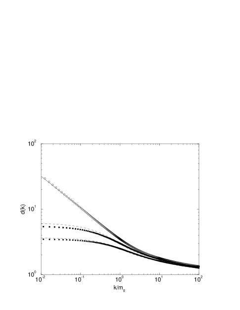
FIG. 4.: Solution for the expectation value of the FP operator $d(k)$. The two lower dashed lines correspond to analytical, approximate solution with $d(m_{g})=2.5$ (lower) and $d(m_{g})=3$ (higher). Boxes correspond to a full numerical solution for the corresponding values of $d(m_{g})$. The numerical solution close to the critical point is shown by the open circles. The solid line corresponds to a fit to this numerical solution using the formula in Eq. (116)

The numerical solution near the critical point has been fit to the formula

$$d(k)=\left\{\begin{array}[]{cc}d_{c}\left({m_{g}\over k}\right)^{a_{d}}&\mbox{ for }k\leq m_{g},\\ d_{c}\left({{\log(1+b_{d})}\over{\log(k^{2}/m_{g}^{2}+b_{d})}}\right)^{c_{d}}&\mbox{ for }k\geq m_{g}.\end{array}\right.$$ (116)

The fit yields $d_{c}=3.5$, $a_{d}=0.48$, $b_{d}=1.41$ and $c_{d}=0.4\;$ verifying the accuracy of the approximate analytical solution. Fig. 5 shows the Coulomb kernel function $f(k)/f(m_{g})$ for $d(m_{g})=2.5$ and $3.0$. Again, for $d(m_{g})<d_{c}$ the solution saturates at low momentum and the analytical approximation is quite accurate. The solution at the critical point is compared with

$$f(k)/f(m_{g})=\Bigg{\{}\begin{array}[]{cc}\left({m_{g}\over k}\right)^{a_{f}}&\mbox{ for }k\leq m_{g},\\ \left({{\log(1+b_{f})}\over{\log(k^{2}/m_{g}^{2}+b_{f})}}\right)^{c_{f}}&\mbox{ for }k\geq m_{g}.\end{array}$$ (117)

The fit yields, $a_{f}=0.97$, $b_{f}=0.82$ and $c_{f}=0.62$. The low momentum behavior is found to be more enhanced than in the approximate analytical solution. The two fits to the numerical solutions for $d$ and $f$ result in the following expression for the Coulomb kernel $V(k)=f(k)d^{2}(k)/k^{2}$:

$$k^{2}V(k)/f(m_{g})=\left\{\begin{array}[]{cc}(3.50)^{2}\left({m_{g}\over k}\right)^{1.93}&\mbox{ for }k\leq m_{g},\\ 8.07\log^{-0.80}(k^{2}/m_{g}^{2}+1.41)\log^{-0.62}(k^{2}/m_{g}^{2}+0.82)&\mbox{ for }k\geq m_{g}\end{array}\right..$$ (118)

FIG. 5.: $f(k)/f(m_{g})$. Curves as in Fig. 4. The numerical solution near the critical point (open circles) is fit to the formula given by Eq. (117) (solid line).

At low momenta the effective coupling $\alpha_{\rm eff}(k)$ (defined through Eq. (105)) behaves very nearly as $1/k^{2}$. The fact that the power is not exactly $-2$ may be due to discretization error (a finer momentum grid does indeed bring the coefficient closer to $-2$) or the truncations employed in deriving the gap equations. In any event, as will be shown later the difference (roughly 3.5%) is completely negligible with regards to phenomenology.

Assuming linear confinement ($2a_{d}+a_{f}=2$) gives [13]

$$6\pi b=(3.5)^{2}m_{g}^{2}.$$ (119)

Inserting the quark model value for the string tension, $b=0.18$ GeV² yields $m_{g}\approx 530$ MeV. Alternatively, lattice string tensions are typically $0.26$ GeV²[22], giving $m_{g}\approx 630\mbox{ MeV}$. These estimates of the scale are in accord with lattice computations of the adiabatic hybrid surfaces (thus is discussed further in Sec. IV.A) and with old glueball phenomenology[23].

The numerical and ansatz solutions for the gap function are shown in Fig. 6. We note the remarkable accuracy of the simple ansatz for $\omega$, the main difference being the smooth transition through the intermediate momentum region. Notice also that $\omega$ approaches $k$ very rapidly for large momentum.

FIG. 6.: Comparison of the analytical approximation to $\omega(k)$ (dashed line) and the full numerical solution (solid line).

Finally, the numerical stability of the solutions have been tested by varying the number of grid points. Of course this also tests the de facto numerical cutoff dependence of the results. The results are shown in Fig. 7. We find that the numerical results are stable to within a percent. Notice that this also confirms that all UV divergences have been properly subtracted.

FIG. 7.: Numerical solution for $d(k)$ near the critical point for $192$ (circles), $288$ (triangles) and $384$ (diamonds) grid points.

F Higher Order Terms

We now address the issue of the neglected terms in the coupled gap equations. These arise, for example, from truncation of the rainbow-ladder sums, higher order corrections to the Coulomb vacuum energy, and from the terms generated by the Faddeev-Popov determinant ${\cal J}$.

1 Vertex Corrections

The truncation to the rainbow-ladder resummation for the Faddeev-Popov operator and the Coulomb kernel ignores higher order, ${\cal O}(d^{n})$, $n\geq 2$ corrections to the triple Coulomb-transverse-gluon vertex. Using the approximate analytical solutions for $d(k)$ and $\omega(k)$ we estimate these contributions by evaluating the ${\cal O}(d^{2})$ correction. From Eq. (51) it follows that the lowest order correction to the bare vertex is given by

$$\delta\Gamma^{c}_{i}({\bf k},{\bf q},{\bf k}-{\bf q})={N_{c}\over 2}\int{{d{\bf l}}\over{(2\pi)^{3}}}{{[({\bf k}+{\bf l})\cdot\delta_{T}({\bf q})]^{i}[{\bf k}\cdot\delta_{T}({\bf l})({\bf k}+{\bf l}-{\bf q})]}\over{2\omega({\bf l})}}{{d({\bf k}+{\bf l})}\over{({\bf k}+{\bf l})^{2}}}{{d({\bf k}+{\bf l}-{\bf q})}\over{{\bf k}+{\bf l}-{\bf q})^{2}}}T^{c}.$$ (120)

We have evaluated this integral numerically and found that for all values of the external momenta the correction does not exceed a few percent.

2 Second and Fourth Order Corrections to the Coulomb Kernel

Recall that an operator product expansion for the Coulomb kernel has been defined in Sec. II.E, Eq. (46). We now employ the Swift equation (36) and the operator expansion of the Faddeev-Popov operator Eq. (42) to derive an explicit expression for the terms in that expansion:

$$K^{ab}({\bf k},{\bf p};{\bf A}) = \delta({\bf k}+{\bf p})\delta^{ab}K^{(0)}({\bf k})+igf^{acb}\left[K^{(0)}({\bf p})D^{(0)}({\bf k})+D^{(0)}({\bf p})K^{(0)}({\bf k})\right]:{\bf A}^{c}({\bf p}+{\bf k})\cdot{\bf p}:+$$ (121)

$$+ \ldots+(i)^{n}f^{ac_{1}e_{1}}\ldots f^{e_{n-1}c_{n}b}{d\over dg}\left[g^{n+1}D^{(0)}({\bf p})D^{(0)}({\bf p}-{\bf s}_{1})\cdots D^{(0)}({\bf p}-\sum_{\ell=1}^{n}{\bf s}_{\ell})\right]$$ (123)

$$\delta({\bf p}+{\bf k}-\sum_{\ell=1}^{n}{\bf s}_{\ell}):{\bf A}^{c_{1}}({\bf s}_{1})\cdot{\bf p}\ldots{\bf A}^{c_{n}}({\bf s}_{n})\cdot({\bf p}-\sum_{\ell=1}^{n-1}{\bf s}_{\ell}):$$

The term in the expansion of $K$ which contains $n$ gluons is weighted by a product of $n-1$ factors of $D^{(0)}$ and a single factor of $K^{(0)}$. The additional contributions to the VEV of the Hamiltonian discussed in Sec. II.E, ${\cal E}^{(2)}_{C}$ and ${\cal E}^{(4)}_{C}$, come from terms with a product of $n=2$ and $n=4$ normal ordered gluon fields $:{\bf A}^{n}:$ respectively. These are the only contributions which have a nonzero VEV after combining with the charge densities. The contribution to the gap equation is then obtained by taking the derivative of the VEV with respect to $\omega$. As was discussed earlier, an alternative method to derive the gap equation is to require that the off-diagonal (proportional to $\alpha^{{\dagger}}\alpha^{{\dagger}}$ or $\alpha\alpha$) portions of the one-body operators vanish. The second method would indicate that terms with $n=6$, $\rho:{\bf A}^{6}:\rho$, contribute to the gap equation as well since the four gluon fields from the two charge densities can contract with the fields from the kernel leading to an operator proportional to $:{\bf A}^{2}:$. As discussed in Sec. II.E, the apparent difference in these two procedures is resolved if one notices that there are contributions to the gap equation which arise from the implicit dependence of the Coulomb kernel on $\omega$. In the second method, the contribution which would be associated with the $n=6$ term in the operator product expansion of $K$ is identical to the one from the derivative of the kernel in the $n=4$ term contribution to the VEV. This was denoted ${\cal E}^{(4),K}_{C}$ in Sec. II.E. Similarly the term referred to as ${\cal E}^{(0),K}_{C}$ in the discussion preceding Eq. (LABEL:gapgen) is identical to the contribution from the $n=2$ term when the fields from the charge densities are contracted with each other.

Adding all these pieces together yields,

$$\omega^{2}(q)-\omega(\mu)^{2}= q^{2}+[{\cal E}^{(0),\omega}_{C}(q)]+[{\cal E}^{(0),K}_{C}(q)+{\cal E}^{(2),\omega}_{C}(q)]+[{\cal E}^{(2),K}_{C}(q)+{\cal E}^{(4),\omega}_{C}(q)]$$ (125)

$$+[{\cal E}^{(4),K}_{C}(q)]-(q\to\mu).$$

The four terms in the brackets are ${\cal O}(d^{2})$, ${\cal O}(d^{4})$, ${\cal O}(d^{6})$ and ${\cal O}(d^{8})$ respectively; no other corrections exist. We test the importance of the higher order terms by computing the ${\cal O}(d^{4})$ correction to the truncated gap equation.

FIG. 8.: ${\cal O}(d^{4})$ contributions to the gap function from ${\cal E}^{(2),\omega}_{C}$.

An example of a diagram contributing to ${\cal E}^{(2),\omega}_{C}$ is given in Fig. 8. The explicit expressions for ${\cal E}^{(0),K}_{C}$ and ${\cal E}^{(2),\omega}_{C}$ are given below.

$${\cal E}^{(0),K}_{C}(q) = {{N_{c}^{2}}\over{8}}\int{{d{\bf k}}\over{(2\pi)^{3}}}{{d{\bf p}}\over{(2\pi)^{3}}}\left[{{\omega(k)}\over{\omega(p)}}-1\right]Tr[\delta_{T}(\hat{\bf p})\delta_{T}(\hat{\bf k})][({\bf k}+{\bf p})\delta_{T}(\hat{\bf q})({\bf k}+{\bf p})]$$ (127)

$$\times\left[{{f({\bf k}+{\bf p})d^{2}({\bf k}+{\bf p})d({\bf k}+{\bf p})d({\bf k}+{\bf p}+{\bf q})+perm.}\over{({\bf k}+{\bf p})^{2}({\bf k}+{\bf p})^{2}({\bf k}+{\bf p}+{\bf q})^{2}}}\right]$$

and

$${\cal E}^{(2),\omega}_{C}(q) = {{N_{c}^{2}}\over{16}}\int{{d{\bf k}}\over{(2\pi)^{3}}}{{d{\bf p}}\over{(2\pi)^{3}}}\left[1-{{\omega^{2}(q)}\over{\omega(k)\omega(p)}}\right][({\bf q}+{\bf k})\delta_{T}(\hat{\bf p})\delta_{T}(\hat{\bf q})\delta_{T}(\hat{\bf k})({\bf q}+{\bf p})]$$ (132)

$$\times\left[{{f({\bf q}+{\bf k}+{\bf p})d^{2}({\bf q}+{\bf k}+{\bf p})d({\bf q}+{\bf k})d({\bf q}+{\bf p})+perm.}\over{({\bf q}+{\bf k}+{\bf p})^{2}({\bf q}+{\bf k})^{2}({\bf q}+{\bf p})^{2}}}\right]$$

$$+{{N_{c}^{2}}\over{8}}\int{{d{\bf k}}\over{(2\pi)^{3}}}{{d{\bf p}}\over{(2\pi)^{3}}}\left[1-{{\omega(k)}\over{\omega(p)}}\right]({\bf k}-{\bf q})\delta_{T}({\bf p})\delta_{T}({\bf k})\delta_{T}({\bf q})({\bf p}-{\bf k})$$

$$\times\left[{{f({\bf p}-{\bf k})d^{2}({\bf p}-{\bf k})d({\bf p}-{\bf k}+{\bf q})d({\bf k}-{\bf q})+perm.}\over{({\bf p}-{\bf k})^{2}({\bf p}-{\bf k}+{\bf q})^{2}({\bf k}-{\bf q})^{2}}}\right],$$

Here the permutations refer to the other two ways of arranging the argument of $fd^{2}$ in $f(1)d^{2}(1)\cdot d(2)\cdot d(3)$.

Including these terms in the gap equations modifies the results for $d$ and $f$ by strengthening the IR enhancement somewhat. The result for the gap function is shown in Fig. 9. As expected, the change at higher momenta is minimal. However, we see that the ${\cal O}(d^{4})$ terms do not modify $\omega$ at low momentum either. This is because ${\cal E}^{2,\omega}$ and ${\cal E}^{0,K}$ depend on the combination $\omega(p_{1})/\omega(p_{2})-1$ which suppresses them in the IR limit (${\bf p}_{1}={\bf p}_{2}$). Our results are compared to lattice computations in Sec. IV.A. We stress that the result of Fig. 9 should be considered preliminary because there are other ${\cal O}(d^{4})$ corrections (see the next subsection) that have not yet been included.

FIG. 9.: Normalized instantaneous transverse gluon propagator, $1/2\omega(k)$. The dashed line is the solution to the leading order gap equation of Eq. (92); the solid line includes ${\cal O}(d^{4})$ corrections.

The computation of the ${\cal O}(d^{6})$ and ${\cal O}(d^{8})$ corrections is progressively more difficult and is currently under investigation. These require the numerical solution of a self-consistent equation involving at least 8-dimensional integrals. However, since the ${\cal O}(d^{4})$ corrections are small we expect these higher order terms not to change the results significantly.

3 Faddeev-Popov Contributions

We now discuss the corrections due to the Faddeev-Popov determinants ${\cal J}$. We calculate the contribution to the gap equation for the determinant present in the kinetic part of the Hamiltonian, through the ${\cal J}^{-1/2}\Pi{\cal J}^{1/2}$ operators. This is given by

$${1\over 2}\int d{\bf x}{\cal J}^{-1/2}\Pi^{a}({\bf x}){\cal J}\Pi^{a}({\bf x}){\cal J}^{1/2}={1\over 2}\int d{\bf x}\Pi^{a}({\bf x})\Pi^{a}({\bf x})+V_{A}.$$ (134)

Similarly, $V_{B}$ is defined via the relation (see Eq. 21)

$$H_{C}={1\over 2}\int d{\bf x}d{\bf y}\rho^{a}(x)K_{ab}({\bf x},{\bf y};{\bf A})\rho^{b}(y)+V_{B}.$$ (135)

A direct computation yields

$$V_{A}= {g^{2}\over 4}\int d{\bf x}f^{abc}f^{aef}\delta_{T}({\mbox{\boldmath$\nabla$}}_{\bf x})_{ij}\langle{\bf x}b|({\mbox{\boldmath$\nabla$}}\cdot D)^{-1}|{\bf x},c\rangle\stackrel{{\scriptstyle\leftarrow}}{{{\mbox{\boldmath$\nabla$}}_{\bf x}}}_{j}\delta_{T}({\mbox{\boldmath$\nabla$}}_{\bf x})_{ik}\langle{\bf x}e|({\mbox{\boldmath$\nabla$}}\cdot D)^{-1}|{\bf x},f\rangle\stackrel{{\scriptstyle\leftarrow}}{{{\mbox{\boldmath$\nabla$}}_{\bf x}}}_{k}$$ (136)

$$- {g^{2}\over 8}\int d{\bf x}f^{abc}f^{aef}\delta_{T}({\mbox{\boldmath$\nabla$}}_{\bf x})_{ij}\langle{\bf x}b|({\mbox{\boldmath$\nabla$}}\cdot D)^{-1}|{\bf x},f\rangle\stackrel{{\scriptstyle\leftarrow}}{{{\mbox{\boldmath$\nabla$}}_{\bf x}}}_{j}\delta_{T}({\mbox{\boldmath$\nabla$}}_{\bf x})_{ik}\langle{\bf x}e|({\mbox{\boldmath$\nabla$}}\cdot D)^{-1}|{\bf x},c\rangle\stackrel{{\scriptstyle\leftarrow}}{{{\mbox{\boldmath$\nabla$}}_{\bf x}}}_{k}.$$ (137)

or in momentum space

$$V_{A}= -{1\over 8}\int{d^{3}k\over(2\pi)^{3}}{d^{3}p\over(2\pi)^{3}}{d^{3}q\over(2\pi)^{3}}D^{ac}({\bf q},{\bf q}+{\bf k})D^{de}({\bf p}+{\bf k},{\bf p})f^{bca}f^{bed}[{\bf q}\delta_{T}({\bf k}){\bf p}]$$ (140)

$$+{1\over 4}\int{d^{3}k\over(2\pi)^{3}}{d^{3}p\over(2\pi)^{3}}{d^{3}q\over(2\pi)^{3}}D^{ac}({\bf q},{\bf k}+{\bf p})D^{de}({\bf p},{\bf q}-{\bf k})f^{bcd}f^{bea}[{\bf q}\delta_{T}({\bf k}){\bf p}]$$

where $D^{ac}(p,k)=\langle a{\bf p}|{g\over\nabla\cdot D}|c{\bf k}\rangle$. We note that $V_{A}$ is similar to Christ and Lee’s $V_{1}$; however, it is not identical because we have not Weyl ordered the Hamiltonian.

Using the operator product expansion for the FP operator, these lead to terms proportional to $:{\bf A}^{2}:$ which add to the gap equation the following contribution

$${\cal E}^{2,\omega}_{FP}(q)= {{N^{2}_{C}}\over 16}\int{{d{\bf k}}\over{(2\pi)^{3}}}{{d{\bf p}}\over{(2\pi)^{3}}}{{d({\bf k}+{\bf q})}\over{({\bf k}+{\bf q})^{2}}}{{d({\bf k})}\over{{\bf k}^{2}}}[{\bf k}\delta_{T}({\bf q}){\bf p}]^{2}{{d({\bf p}+{\bf q})}\over{({\bf p}+{\bf q})^{2}}}{{d({\bf p})}\over{{\bf p}^{2}}}$$ (142)

$$- {{N^{2}_{C}}\over 16}\int{{d{\bf k}}\over{(2\pi)^{3}}}{{d{\bf p}}\over{(2\pi)^{3}}}{{d({\bf k}+{\bf q})}\over{({\bf k}+{\bf q})^{2}}}{{d({\bf k})}\over{{\bf k}^{2}}}[{\bf k}\delta_{T}({\bf q}){\bf p}][({\bf k}+{\bf q})\delta_{T}({\bf p}+{\bf q}+{\bf k})({\bf p}+{\bf q})]{{d({\bf p}+{\bf q})}\over{({\bf p}+{\bf q})^{2}}}{{d({\bf p})}\over{{\bf p}^{2}}}$$ (143)

$$- {{N^{2}_{C}}\over 4}\int{{d{\bf k}}\over{(2\pi)^{3}}}{{d{\bf p}}\over{(2\pi)^{3}}}\left({{d({\bf k})}\over{{\bf k}^{2}}}\right)^{2}[{\bf k}\delta_{T}({\bf p}){\bf k}][{\bf k}\delta_{T}({\bf q}){\bf k}]{{d({\bf k}+{\bf q})}\over{({\bf k}+{\bf q})^{2}}}{{d({\bf k}+{\bf p})}\over{({\bf k}+{\bf p})^{2}}}$$ (144)

The contribution of $V_{A}$ to the gap equation is IR-finite but UV-divergent thus will modify the gluon mass counterterm. A detailed numerical study of the full $O(d^{4})$ corrections to the gap equation will be presented elsewhere.

IV Discussion

As demonstrated in the previous section, the asymptotic behavior of the numerical solution to the gap equations is $V(k)\sim 1/k^{4}$, it thus appears that the methodology advocated in this paper is capable of describing quark confinement. The appearance of the confinement phenomenon hinges crucially on the choice of the variational vacuum which we use to construct the quasiparticle basis and on realizing that this choice also affects the interaction between these quasiparticles via the summed expression for the instantaneous Coulomb kernel. We now examine the implications of this success on confinement and the Gribov ambiguity.

A The Confinement Potential

The requirement that the gluon mass gap function $\omega(k)$ be cutoff independent gives rise to a mass scale which we call the gluon mass, $m_{g}$. The value of $\omega$ at a particular momentum scale, say $k=0$ serves then as the underlying mass parameter of the theory. At the critical coupling $d_{c}$ the only free parameters in the gluon sector are $Z_{K}(\mu)$ and the momentum scale itself, $m_{g}=\omega(0)$. Nonperturbative renormalization may be carried out by requiring that the Coulomb kernel reproduce the static $Q\bar{Q}$ heavy quark potential as seen on the lattice (recall that $V_{Q\bar{Q}}$ is a renormalization group invariant quantity). In our approach this potential is given by

$$H_{QCD}|Q(r/2),{\bar{Q}}(-r/2)\rangle=V_{Q\bar{Q}}(r)|Q(r/2),{\bar{Q}}(-r/2)\rangle,$$ (145)

In pure QCD, i.e. ignoring light flavors, the above eigenstate can be expanded in terms of multigluon states constructed from the quasiparticle operators acting on the $|\omega\rangle$ vacuum. Schematically,

$$|Q(r/2),{\bar{Q}}(-r/2)\rangle=\sum_{n=0}\psi_{n}(\alpha^{\dagger})^{n}b^{{\dagger}}(r/2)d^{{\dagger}}(-r/2)|\omega\rangle.$$ (146)

where the quark creation operators refer to static sources. The Hamiltonian mixes states differing by gluon number; however, one expects that the mixing between such states to be suppressed by energy denominators due to the gluon mass gap, $\omega(0)\neq 0$ (this is discussed in much more detail in Sec. V.A). This mass gap can be estimated from the difference between the lowest and excited adiabatic $Q\bar{Q}$ potentials which have been calculated on the lattice[22]. One finds that this difference is $\Delta V(r\sim 1\ \mbox{fm})\sim 600-800\ \mbox{MeV}$. This is a natural estimate for $\omega(k)$ at low momenta. The implication is that the static ground state heavy quark potential may be accurately computed by ignoring extra gluonic excitations in the heavy quark system. (A calculation of the excited adiabatic potentials will be presented elsewhere.) Thus, to good accuracy, the static heavy quark potential $V(r)$ is given by

$$V_{Q\bar{Q}}(r)=-C_{F}V(r)=-C_{F}\int{{d{\bf k}}\over{(2\pi)^{3}}}e^{i{\bf k}\cdot{\bf x}}{{f(k)d^{2}(k)}\over{{\bf k}^{2}}}\equiv-C_{F}\int{{d{\bf k}}\over{(2\pi)^{3}}}e^{i{\bf k}\cdot{\bf x}}{{4\pi\alpha_{\rm eff}(k)}\over{{\bf k}^{2}}}.$$ (147)

It is useful to return to the approximate analytical solutions to the truncated renormalized gap equations of Sec. III.D to illustrate how the different parameters enter. We have seen that at the critical point $d_{c}$ the solutions for the Faddeev-Popov operator and the Coulomb kernel are

$$d(k)=\left\{\begin{array}[]{cc}d(m_{g})\left({{m_{g}}\over k}\right)^{1\over 2}&\mbox{ for }k\leq m_{g}\\ {{d(m_{g})}\over{\sqrt{1+{3\over 5}\log{{k^{2}}\over{m_{g}}^{2}}}}}&\mbox{ for }k\geq m_{g}\end{array}\right.$$ (148)

and

$$f(k)=\left\{\begin{array}[]{cc}f(m_{g})\left({{m_{g}}\over k}\right)^{3\over 4}&\mbox{ for }k\leq m_{g}\\ {{f(m_{g})}\over{\sqrt{1+{3\over 5}\log{{k^{2}}\over{m_{g}}^{2}}}}}&\mbox{ for }k\geq m_{g}\end{array}\right.$$ (149)

Since $d(m_{g})=d_{c}\sim 3.4414$ is fixed, the potential has only two free parameters, the overall strength determined by $f(m_{g})$ and the mass scale set by $m_{g}=\omega(0)$. These may be determined by comparing with lattice computations of the Wilson loop. One finds $f(m_{g})\sim 1.0$ and $m_{g}\approx 1.8/r_{0}$. Here $r_{0}$ is the Sommer parameter of lattice gauge theory which is determined to be roughly 1/430 MeV^-1. Thus $m_{g}\approx 720\mbox{ MeV}$.

The same procedure may be followed for the numerical solution to the gap equation. Good agreement with the lattice static potential is obtained by choosing $f(m_{g})=1.41$ and $m_{g}=1.4/r_{0}=600$ MeV. The minimum in parameter space is fairly broad, for example $f(m_{g})=1.09$ and $m_{g}=1.6/r_{0}=690$ MeV provides nearly as good a description of $V_{Q\bar{Q}}$. The resulting potential (after numerically Fourier transforming to configuration space) is presented in Fig. 10. One sees that the numerically obtained static quark potential provides a reasonable facsimile of the lattice potential. This somewhat surprising result provides a posteriori support for the methodology advocated here.

FIG. 10.: Static $Q{\bar{Q}}$ ground state potential. The solid line is the full numerical solution for $f(m_{g})=1.41$ and $m_{g}=1.4/r_{0}=600\mbox{ MeV}$. Data are taken from Ref. [22].

B The Gribov-Zwanziger Horizon and the Gap Function

As mentioned in Sec. II.B, the Gribov problem may be resolved by selecting a single gauge copy from the ensemble of Gribov copies by imposing the horizon condition of Eq. (23). Furthermore, Zwanziger [7] has shown that the restriction to the fundamental modular region imposed by the horizon term is equivalent to having a low-momentum enhancement in the Faddeev-Popov operator over the perturbative $1/k^{2}$ behavior. This enhancement takes the form

$${1\over{D^{(0)}(k)}}=k_{i}k_{j}(\Sigma(0)_{ij}-\Sigma(k)_{ij}),$$ (150)

where $\Sigma$ is a regular function at the origin. Such a behavior is clearly an indication of confinement [5], since the FP operator determines the static potential between color sources (cf. Eq. (21) or Eq. (36)). Comparing Eq. (150) with Eq. (47) shows that this is equivalent to the statement that $d(k)$ is singular at the origin,

$$\lim_{k\to 0}1/d(k)\to 0.$$ (151)

The behavior of $d$ at small momenta depends on one integration constant, $d(\mu)$. As we have shown earlier, $d(k)$ approaches a finite value as $k\to 0$ except when $d(\mu)=d_{c}$ where the Gribov-Zwanziger singularity develops.

It is possible that the saturation of $d(k)$ to finite values when $d(\mu)<d_{c}$ is an artefact of the rainbow-ladder approximation – we leave this as a matter of future investigation. For the present we simply require that the theory give rise to an enhancement of the FP operator at small momentum, this boundary condition then selects the coupling $d(\mu)=d_{c}$.

In Ref. [7] the enhancement in the FP operator was obtained by adding the horizon term to the Hamiltonian via a Lagrange multiplier. The VEV of the new Hamiltonian was then computed in the bare vacuum, i.e with $\omega(k)=k$; however, the horizon terms adds a mass term through an effective ${\bf A}^{2}$ operator whose strength is determined by the expectation value of the FP operator. This term has the effect of enhancing $d(k)$ for small $k$. The equivalent of Eq. (64) was then solved and the Coulomb operator was approximated by the square of the FP operator.

In our approach the horizon condition was used to justify the expansion of the FP operator in a power series in $g{\bf A}$. The resulting expressions for the FP operator were summed in the presence of a nontrivial mean field background (the variational vacuum) with the aid of the rainbow approximation producing IR enhanced FP and Coulomb VEVs. The success of this procedure demonstrates that the explicit effects of the horizon term may be ignored if one is willing to develop the quasiparticle spectrum and interaction self consistently.

To further test this mechanism for realizing the Gribov-Zwanziger confinement scenario we compare our result for the gap function to that computed by Cucchieri and Zwanziger in SU(2) lattice gauge theory[24]. In that paper, the authors measure the transverse and instantaneous gluon propagators in ‘minimal Coulomb gauge’. They compare the numerical results to a functional form proposed by Gribov[5]:

$$D^{tr}(k)={1\over{2E_{G}(k)}},\;E_{G}(k)={1\over k}\sqrt{k^{4}+M_{G}^{4}}.$$ (152)

We call the scale appearing in this relationship, the Gribov mass, $M_{G}$. Cucchieri and Zwanziger found the the computed instantaneous transverse propagator agreed very well with this functional form but does not reproduce the normalization.

As discussed earlier, in our approach the transverse gluon propagator is suppressed due to an infrared singularity in the one-body gluon operator. Explicitly, the one body operator in the quasiparticle basis is given by

$$H_{one-body}=\sum_{\lambda,c}\int{{d{\bf k}}\over{(2\pi)^{3}}}E(k)\alpha^{{\dagger}}({\bf k},\lambda,c)\alpha({\bf k},\lambda,c)$$ (153)

with

$$E(k)=\omega(k)\left[1+{N_{c}\over 4}\int{{d{\bf q}}\over{(2\pi)^{3}}}{{f({\bf k}-{\bf q})d^{2}({\bf k}-{\bf q})}\over{({\bf k}-{\bf q})^{2}}}{{1+({\hat{\bf k}}\cdot{\hat{\bf q}})^{2}}\over{\omega(q)}}\right].$$ (154)

The low-momentum enhancement of the kernel makes the integral infrared singular. Thus, as expected, gluons do not propagate.

We note that the equal time transverse gluon propagator is not determined by $E(k)$ but by $\omega(k)$

$$D^{tr}(x)=\lim_{t\to 0}\langle\omega|T[{\bf A}^{a}({\bf x},t){\bf A}^{b}({\bf 0},0)]|\omega\rangle=\delta^{ab}\int{{d{\bf k}}\over{(2\pi)^{3}}}{{\delta_{T}({\bf k})}\over{2\omega(k)}}e^{i{\bf k}\cdot{\bf x}}.$$ (155)

We have seen that the gap function obtained in Sec. III is rather flat at small momenta, even when some $d^{4}$ corrections are incorporated into the gap equation. This is inconsistent with the lattice calculation for the same quantity, but as shown above, not inconsistent with the Gribov confinement scenario. The disagreement with lattice may be due to the use of the rainbow-lattice approximation and is being investigated. It is worth noting however that the effective gluon mass found by comparison to the $Q{\bar{Q}}$ potential (or alternatively the $D^{00}$ gluon propagator) is consistent with that found in the Coulomb gauge lattice calculations.

V Implications for the Constituent Quark Model and Phenomenology

We now turn to an examination of the implications of the results presented here on the phenomenology of hadrons. Since this depends crucially on the explicit definition of hadronic states, we begin by searching for an efficient way to construct hadrons by specifying a new constituent quark model of QCD. The phenomenology of confinement is then analysed in light of the results of the last two sections. We conclude with a clarification of several open issues in the old constituent quark model and present a justification for the surprising efficacy of the quark model for light hadrons.

A Constructing Hadrons

It is clear that constructing hadrons from the basis of free quasiparticles is futile if it is done perturbatively. A simple and natural way to avoid this pitfall is to choose a convenient form of $H_{0}$ and diagonalise it nonperturbatively to obtain a basis of color singlet bound states. Bound state perturbation theory may then be employed to systematically include the effects of $H_{int}$. In our case the natural assignment for these operators is

$$H_{0}=\int\psi^{\dagger}\left(-i{\mathchoice{{\hbox{\boldmath$\displaystyle\alpha$}}}{{\hbox{\boldmath$\textstyle\alpha$}}}{{\hbox{\boldmath$\scriptstyle\alpha$}}}{{\hbox{\boldmath$\scriptscriptstyle\alpha$}}}}\cdot{\mbox{\boldmath$\nabla$}}+\beta m\right)\psi+{1\over 2}\int d{\bf x}{\mbox{\boldmath$\Pi$}}^{2}-{1\over 2}\int d{\bf x}{\bf A}{\mbox{\boldmath$\nabla$}}^{2}{\bf A}+{1\over 2}\int d{\bf x}d{\bf y}\,\rho^{a}({\bf x})K^{(0)}({\bf x}-{\bf y})\rho^{a}({\bf y})$$ (156)

and

$$H_{int} ={1\over 2}\int d{\bf x}\left[{\bf B}^{2}+{\bf A}{\mbox{\boldmath$\nabla$}}^{2}{\bf A}\right]-g\int\psi^{\dagger}{\mathchoice{{\hbox{\boldmath$\displaystyle\sigma$}}}{{\hbox{\boldmath$\textstyle\sigma$}}}{{\hbox{\boldmath$\scriptstyle\sigma$}}}{{\hbox{\boldmath$\scriptscriptstyle\sigma$}}}}\cdot{\bf A}\psi+V_{A}+V_{B}+$$ (157)

$$+{1\over 2}\int d{\bf x}d{\bf y}\,\rho^{a}({\bf x})\left[K^{ab}({\bf x}-{\bf y};{\bf A})-\delta^{ab}K^{(0)}({\bf x}-{\bf y})\right]\rho^{b}({\bf y})$$ (158)

The general philosophy is clear – $H_{0}$ generates hadronic bound states; $H_{int}$ incorporates the corrections to these states due to transverse gluon exchange, three and four gluon interactions, and higher order contributions from the FP determinant and instantaneous confinement potential. It is worth stressing that $H_{0}$ is still a field theory and hence is considerably tougher to solve than old fashioned quantum mechanical quark models. But there are substantial advantages to adopting this approach. Foremost is that $H_{0}+H_{int}$ is QCD. Furthermore, $H_{0}$ is relativistic and incorporates gluonic degrees of freedom. Thus it is possible to examine glueballs, hybrids, and other gluonic phenomena in a coherent fashion. The utility of the rearrangement made in Eq. (158) lies in the use of the variational vacuum to construct a phenomenologically viable basis of quasiparticles. This has the direct effect of greatly improving the Fock space convergence of any observable. As we have seen, it also automatically generates the correct static potential upon which to construct hadrons. We have previously mentioned that $H_{0}$ generates states which are infrared divergent if they are not color singlets (hence these are removed from the spectrum). Conversely, all color singlets are IR finite. Thus the basis generated by $H_{0}$ contains no spurious color nonsinglet states which would have to be removed by laborious iteration of $H_{int}$ and, in fact, is expected to provide a reasonably accurate starting point for hadronic spectrum computations. As a practical note, the physics of the variational vacuum may be accurately approximated by simply using dressed quarks and gluons when constructing hadrons. The constituent masses are roughly 200 MeV and 600-800 MeV respectively. Finally, the spectrum generated by $H_{0}$ is spin averaged in the sense that it only incorporates spin effects from relativistic corrections to the Coulomb potential. Full spin splittings come from $H_{int}$.

An important implication of this approach is that the rapid convergence of the constituent quark model Fock space expansion has a natural and simple explanation. All of the corrections induced by $H_{int}$ (for nonexotic states) involve the transfer of a virtual transverse gluon. Since these are quasiparticles in the variational vacuum, the relevant perturbative diagrams are suppressed by the mass gap between the regular and hybrid states. This simple feature of QCD in Coulomb gauge has important phenomenological consequences. For example, it implies that the Fock space expansion converges quickly because state mixing involves the creation of massive gluonic (or quark) quasiparticles. Recently, lattice data has appeared which confirms this picture. Duncan et al.[25] have constructed a simple relativistic quark model of $B$ mesons by considering a light relativistic quark (with kinetic energy $\sqrt{k^{2}+m^{2}}$) moving in the lattice $\Upsilon$ potential. Detailed comparison with lattice $B$ data demonstrated the high accuracy of the model. The point which is relevant for our discussion is that the lattice $\Upsilon$ interaction (recall that this is equivalent in principle and in practice to $K^{(0)}$) should receive corrections due to the light quark when applied to $B$ mesons; see Fig. 11. The fact that these corrections are not important demonstrates that they are suppressed, in agreement with the above arguments.

FIG. 11.: The leading light quark correction to the confinement potential

B Confinement in the Constituent Quark Model

One of the benefits of Coulomb gauge is that it makes the source of confinement clear: in the heavy quark limit quarks and transverse gluons decouple and the quark-antiquark quark interaction arises solely from the instantaneous Coulomb operator. This rigorous result has several significant implications for hadronic phenomenology.

First we simplify the situation by noting that higher order terms such as shown in Fig. 12 are suppressed due to the arguments espoused in the previous subsection. Thus, the dominate interaction between static color sources is the leading kernel in the Coulomb interaction, $K^{(0)}$. As we have seen, this kernel is essentially identical to the lattice Wilson loop result, so this conclusion is supported a posteriori.

FIG. 12.: Examples of Higher Order Corrections to the Heavy Quark-Antiquark Interaction.

This simple statement carries wide repercussions. For example, a longstanding cornerstone of quark model phenomenology is that confinement is ‘scalar’. What this means is that the interaction between quarks is assumed to be

$${1\over 2}\int\bar{\psi}\psi({\bf x})K({\bf x}-{\bf y})\bar{\psi}\psi({\bf y}).$$ (159)

This form (as opposed to ‘vector’ confinement $\psi^{\dagger}\psi K\psi^{\dagger}\psi$) is supported by a comparison of the predicted spin splittings in heavy quarkonia with data[26]. However, the results presented here make it clear that this conclusion is naive. The interactions between color sources is more complicated than the simple facsimile given in Eq. (159). As we have seen, the leading interaction between quarks is given by $K^{(0)}$ – and this has the form of vector confinement. What is taken as evidence of the scalar nature of confinement is in fact quarkonium spin splittings which are generated by nonperturbative mixing with intermediate hybrid states via $H_{int}$. That this more complicated (and correct) picture may look ‘scalar’ has been shown in Ref. [14]

Another simple conclusion of the picture being developed here is that the confinement potential between color sources scales as the quadratic Casimir. This follows from the observation that the dominant contribution to the confinement potential is given by the leading kernel and that the color structure of this kernel is $K^{(0)}_{ab}=\delta_{ab}K^{(0)}$. The fact that Casimir scaling of the Wilson loop potential has been observed repeatedly[27] may be taken as a successful prediction of our methodology or may be used as further proof that the diagrams of Fig. 12 are suppressed with respect to $K^{(0)}$.

The methodology presented here allows for the resolution of several open, but often ignored, ambiguities in the constituent quark model. For example, it is often stated that the linear potential is built from the exchange of infinitely many gluons. One may then ask why the one gluon exchange potential is retained as an important part of quark model phenomenology. Indeed the split between one gluon exchange color Coulomb and hyperfine forces and the multiexchange linear force is necessarily ambiguous. The resolution to this issue is transparent in Coulomb gauge: ‘one gluon exchange’ is part of $H_{int}$ and is due to noninstantaneous transverse gluon exchange. The instantaneous central portion of the quark model should consist of a linear term in addition to the running resummed ‘Coulomb’ term of Eq. (118). No ambiguity exists because of the separation of instantaneous and transverse degrees of freedom inherent in Coulomb gauge.

Another problem with the old-fashioned CQM has to do with the previously mentioned assumed scalar nature of confinement. Unfortunately, scalar confinement implies that if mesons are bound by a linear potential, baryons are antibound [28]. This is clearly an intolerable situation which is routinely ignored by CQM practitioners. As we have seen, the resolution is that confinement acts as the time component of a vector rather than as a scalar, and no inconsistency exists between mesons and baryons.

C Constituent Gluons and Strong Decays

We illustrate the power of our approach by considering the vexing problem of strong decays in hadronic physics.

The strong decays of hadrons has been, and remains, a mystery of soft QCD. The naive perturbative assumption that the decay proceeds via one gluon dissociation (Fig. 13b) is proven incorrect by direct comparison with experiment[29]. The only reasonably successful phenomenology is provided by the ‘${}^{3}P_{0}$’ model[30], where quark pairs are assumed to appear with vacuum quantum numbers over all space. This is clearly an unacceptable situation, especially given the ubiquity of hadronic decays and the fact that they provide a window into the dynamics of glue at low energy.

We now examine the predictions of the new quark model presented here. To lowest order in $\Lambda_{QCD}/m_{g}$ and to all orders in the coupling, the only diagrams which contribute to meson decay (here all mesons are assumed to have Fock expansions which are dominated by the quasiquark-quasiantiquark components) are shown in Fig. 13. The left figure is contained within $H_{0}$ and is therefore the leading diagram. The central and right figures contribute at ${\cal O}(\Lambda_{QCD}/m_{g})$ and are generated by $H_{int}$.

Diagrams (a) and (b) with perturbative gluons or model potentials in the intermediate states have been previously examined as possible sources of hadronic decays in Ref. [31]. The authors noted that diagram (a) is strongly suppressed with respect to (b) due to momentum routing through the pair production vertex (this diagram is zero in the nonrelativistic limit when a delta function potential is in place. It is strongly suppressed with a $1/q^{4}$ potential). The other class of diagrams considered in Ref.[31] was that generated by a phenomenological scalar interaction given in terms of scalar confinement (cf. Eq. (159)). This is, of course, an ad hoc microscopic realization of the ${}^{3}P_{0}$ model. What was found was that this diagram (like diagram (a) but with scalar as opposed to a vector vertices) was much larger than diagram (b).

FIG. 13.: Leading Order in $1/m_{g}$ Meson Decay Diagrams

These conclusions imply that the ${}^{3}P_{0}$ model would emerge in a natural way from our methodology if diagram (c) produced light quark pairs with scalar quantum numbers. Diagram (c) is generated by the product of $K^{(1)}$ and $H_{qg}$ terms in $H_{int}$ (see Eqs. (20) and (123)) and is roughly given by ${\bf A}\cdot{\mbox{\boldmath$\nabla$}}\psi^{\dagger}\alpha\cdot{\bf A}\psi$. Once the vector potentials are contracted (or better yet, the sum over intermediate hybrid states is made), the resulting operator is of the form $\psi^{\dagger}[{\mbox{\boldmath$\sigma$}}\delta_{T}{\mbox{\boldmath$\nabla$}}]\psi$, very nearly equal to the long-assumed ${}^{3}P_{0}$ vertex. Thus we have obtained a viable microscopic description of hadronic decays. The implications of these observations will be explored in a future publication.

D Light Quarks and the Constituent Quark Model

The utility of the CQM for heavy quarkonium is not in doubt. However, its apparently successful extension to light quark states is unexpected and surprising. We seek to understand this observation in this subsection.

The major feature of light quark physics is spontaneous chiral symmetry breaking. One may regard this as occurring due to the appearance of a quark-antiquark vacuum condensate. The interactions which generate the condensate are typically associated with an effective instanton interaction[32] or the confinement potential[8, 9, 10]. (In our approach the driving kernel would be $K^{(0)}$). Regardless of the particular mechanism which causes attraction in the scalar channel, a massive constituent quark is the necessary outcome. Indeed, while bare quarks may become very light or massless, the relevant quasiparticles saturate at roughly 200 MeV as the bare quark mass is reduced[15, 12]. This, at least partly, explains the apparent success of the nonrelativistic portion of the CQM. The agreement is also enhanced by the empirical accident that the expectation value of $\sqrt{p^{2}+m^{2}}$ is very close to ${\bf p}^{2}/2m_{\rm CQM}$ in typical hadronic states. More important than this; however, is the nature of the central potential itself when the bare quarks are light. As discussed above, effects due to one gluon exchange are suppressed by powers of $\Lambda_{QCD}/m_{g}$. Thus the main effect due to light quarks is the presence of intermediate quark loops in the instantaneous interaction (Fig. 14). These diagrams cause string breaking which is an important feature of QCD. However, as Isgur has argued[33], the main consequence of this is simply to renormalize the string tension. Thus light quark loops have little effect on the phenomenology arising from $H_{0}$. The conclusion is that structure of the new CQM which we have laid out is essentially unchanged for light quarks. Furthermore, even the simple nonrelativistic approximation may retain some validity for massless bare quarks.

FIG. 14.: Light Quark Loop Correction to the Heavy Quark-Antiquark Interaction.

An explicit demonstration of how the CQM may emerge was given in Ref. [12]. This paper assumed a simple contact interaction in place of the full Coulomb kernel. Standard many-body techniques were used to obtain chiral symmetry breaking and constituent (quasiparticle) quarks. It was then demonstrated that the vector meson – pseudoscalar meson mass splitting follows a form essentially identical to that of the CQM hyperfine splitting when considered as a function of the constituent mass. Nevertheless, the mass splitting was clearly driven by chiral symmetry breaking when considered as a function of the current quark mass, thereby demonstrating that the pion may be viewed as both a pseudoGoldstone boson and as a quark-antiquark bound state. The new quark model presented here provides an explicit microscopic realization of the contact model employed in Ref. [12] and it will be of interest to verify the findings of that work.

VI Conclusions

In the paper we propose a new way to organize QCD which is appropriate for low energy hadronic physics. The starting point is chosen to be the QCD Hamiltonian in Coulomb gauge because this gauge is most directly applicable to bound state physics – the degrees of freedom are physical and an instantaneous potential exists. The instantaneous Coulomb potential may be incorporated into $H_{0}$ (as is done in atomic physics) and a viable bound state perturbation theory may be constructed. This simple step already obviates one of the severe problems of perturbative QCD in describing hadronic properties, namely that of ill-defined asymptotic states.

While the division of the QCD Hamiltonian is a simple task, it is essentially meaningless because the degrees of freedom represented in $H_{0}$ are partonic. Thus building bound states would be a frustrating exploration of the depths of Fock space rather than the preliminary step for bound state perturbation theory we desire it to be. The experience provided by the constituent quark model points the way out of the impasse: appropriate (constituent) degrees of freedom must be employed. The problem in the past (cf. constituent quark models, bag models, flux tube models, etc) has been in finding a way to introduce effective degrees of freedom in such a way that the connection to QCD is not destroyed. Herein we present one way to do this which is based on experience gleaned from many-body physics often used in phenomenological models e.g. the Nambu–Jona-Lasinio model[34]. Specifically, a canonical transformation to a quasiparticle basis which is defined with respect to a nontrivial variational vacuum is made. The theory remains QCD but is given in terms of a useful and tractable basis. Although the vacuum state is necessarily an ansatz, this does not vitiate the construction – in principle any basis may be used, we merely seek an efficient one, and the vacuum itself may be systematically improved with standard techniques.

One finds a welcome complication when these ideas are applied to nonabelian gauge theory: the interaction which is needed to define the vacuum ansatz and the quasiparticle spectrum (via the gap equation) itself depends on the vacuum. Thus the fundamental quasiparticle interaction and the quasiparticles themselves are inextricably interdependent. Solving the gap equations requires the evaluation of the specific functional dependence of the quasiparticle interaction on the vector potential. We have chosen to do this within the rainbow ladder approximation. There are several important points to make at this stage: (1) the rainbow ladder approximation may be improved at will, (2) the approximation is accurate in the large $N_{c}$ limit, (3) the approximation is accurate in the infrared limit, (4) the approximation is justified a posteriori. Lastly, although the approximation cannot yield nonperturbative results, true nonperturbative physics may be generated when the resummed kernel is incorporated in the nonlinear coupled gap equations. Doing so reveals a pleasant surprise: the emergence of the confinement phenomenon.

While it is gratifying that color confinement is produced by our approach, this result would be useless if it did not match phenomenology. The fact that the effective quasiparticle potential matches the lattice static quark potential very well points to the general utility of our method. Thus Eqs. (156) and (158) represent much more than a simple reordering of the QCD Hamiltonian. By building $H_{0}$ as an effective Hamiltonian describing the interactions of quasiparticles on a nontrivial vacuum we are able to establish contact with the constituent quark model and derive confinement. That both of these emerge in our formalism bodes well for the future success of $H_{0}$ as a robust starting point for detailed hadronic computations.

An important test of any new method in QCD is its ability to provide insight into a variety of phenomena. We have tried to demonstrate the robustness of our method in this regard. A vital aspect of this robustness is the emergence of $\Lambda_{QCD}/m_{g}$ as an expansion parameter. This provides the justification for gluonic Fock space truncation, for the validity of the leading static Coulomb kernel $K^{(0)}$, and for the applicability of the static kernel to light quarks. Indeed, the method strongly hints as to why the constituent quark model works for light quarks. To summarize, quarks never become truly light (but saturate at constituent masses), the static kernel is not strongly affected by the presence of light quarks, and parameter freedom in the definition of the quark model allows for an accurate reproduction of the relativistic quark kinetic energy and the chirally-driven meson hyperfine splitting.

The ideas we have presented have had a long period of development starting with Gribov’s speculation that confinement may arise naturally when resolving the gauge copy problem. In the early 1980’s Finger and Mandula[8], Adler and Davis[9], and Le Yaouanc et al.[10] all considered the generation of constituent quark masses and spontaneous chiral symmetry breaking with simple (often of the form given in Eq. 159) models of QCD. The issue of renormalization was taken up by these papers and in Refs. [15, 13, 35].

The work which is closest to ours is that of Zwanziger[6] and Swift[21]. As discussed in Sec. IV.B, Zwanziger has shown that the imposition of the horizon condition implies that the Faddeev-Popov propagator is enhanced in the infrared. As we have stressed, an enhancement of the FP propagator is sufficient to cause confinement. In Ref. [6] Zwanziger has shown that adding the horizon term to the Hamiltonian produces an effective gluon mass which in turn induces the desired enhancement of the VEV of the Faddeev-Popov operator. Zwanziger then makes several simplifying assumptions to arrive at an estimate for the Coulomb kernel. Chief among these are an assumed form for the gluon dispersion relation, a simplified version of the Faddeev-Popov propagator integral equation, and the approximation $K\sim d^{2}(k)/k^{2}$. The end results are similar to ours; Zwanziger obtains $d\sim k^{-4/3}$ (we get $k^{-1/2}$) and $V\sim r^{5/3}$. Our analytical approximation gives $V\sim r^{3/4}$ while the numerical solution is very nearly linear.

The work of Swift[21] is very similar to ours in philosophy. In fact our self-consistent equations for the leading rainbow-ladder gap equations, which were derived in the Hamiltonian formalism, agree with those of Ref. [21], which were derived in the Greens function formalism. However, a difference occurs in the renormalization of the mass gap equation: we find that only one subtraction is necessary to render the equation finite. Thus no counterterm proportional to ${\bf A}\nabla^{2}{\bf A}$ is required. This is due to the logarithmic suppression of the potential at large momenta.

The main difference between the current paper and Ref. [21] is in the analysis of the gap equations. We have obtained very good analytic and full numerical solutions to the coupled gap equations. This was not attempted in Ref. [21]; however, the author did examine the small momentum behaviour of the Faddeev-Popov propagator and the Coulomb kernel assuming a particular form for the gap function. His FP and gap functions agree with our analytical estimates, however his solution for the potential has an unexpected imaginary portion. We believe this is due to an approximation which generated a confinement potential which was more singular than $1/k^{4}$.

A preliminary exploration of the work presented here was undertaken in Ref. [13]. This reference neglected the FP determinant and higher order contributions to the gap equation. Furthermore, the full Coulomb kernel was drastically simplified by taking it to be the summation of the one loop expression for $K$. Despite these simplifications and assumptions the resulting potential was similar to that obtained here. This is perhaps an indication of the power of the coupled quasiparticle/vacuum approach.

We regard the present work as a promising start to the construction of a new quark model of the strong interactions in particular with regard to the treatment of gluonic degrees of freedom. Future projects include the evaluation of all $d^{4}$ correction terms to the gap equation which are needed to test the Gribov-Zwanziger gluonic quasiparticle spectral function. We also intend to evaluate a broad swath of the meson, baryon, glueball, and hybrid spectra, and to compute the heavy hybrid adiabatic energy surfaces. The latter two test the utility of the gluonic quasiparticles as effective degrees of freedom and will probe the structure of $K^{(0)}$ and $K^{(1)}$. General considerations (and explicit lattice evidence) lead one to expect that glue behaves as a collective stringlike degree of freedom at large distances. We expect the gluonic quasiparticles to provide a useful description of glue at small (less than 1 fermi) and intermediate (1-2 fermi) scales. It will be interesting to see if the formalism presented here allows for effective stringlike behavior at large distances. Finally, $\eta-\eta^{\prime}$ mixing is a longstanding issue in soft QCD related to the anomaly, vacuum structure, the gluonic content of mesons, and instantons. Examining this problem should prove informative for the further development of the quark sector of our theory.

- [1] S. Capstick et al., Key issues in hadronic physics, hep-ph/0012238.
- [2] J. Schwinger, Phys. Rev. 127, 324 (1962).
- [3] I.B. Khriplovich, Yad. F. 10, 409 (1969).
- [4] N. H. Christ and T. D. Lee, Phys. Rev. D 22, 939 (1980).
- [5] V.N. Gribov, Nucl. Phys. B139, 1 (1978).
- [6] D. Zwanziger, Nucl. Phys. B 485, 185 (1997).
- [7] A. Cucchieri and D. Zwanziger, Phys. Rev. Lett. 78, 3814 (1997).
- [8] J. R. Finger and J. E. Mandula, Nucl. Phys. B 199, 168 (1982).
- [9] S. L. Adler and A. C. Davis, Nucl. Phys. B 244, 469 (1984).
- [10] A. Le Yaouanc, L. Oliver, S. Ono, O. Pene and J. C. Raynal, Phys. Rev. D 31, 137 (1985).
- [11] P.J.A. Bicudo, J.E.F.T Ribeiro, Phys. Rev. D42, 1611 (1990); ibid, 1635 (1990); ibid, D45, 1673 (1992).
- [12] A. P. Szczepaniak and E. S. Swanson, hep-ph/0006306, to appear Phys. Rev. Lett.
- [13] A. P. Szczepaniak and E. S. Swanson, Phys. Rev. D 62, 094027 (2000).
- [14] A. P. Szczepaniak and E. S. Swanson, Phys. Rev. D 55, 3987 (1997).
- [15] A. P. Szczepaniak and E. S. Swanson, Phys. Rev. D 55, 1578 (1997).
- [16] A. P. Szczepaniak, E. S. Swanson, C.-R. Ji, and S. R. Cotanch, Phys. Rev. Lett. 76, 2011 (1996).
- [17] T. D. Lee, Particle Physics And Introduction To Field Theory, (New York, Harwood Academic, 1981).
- [18] D. Zwanziger, Nucl. Phys. B518, 237 (1998).
- [19] L.I. Schiff, Phys. Rev. 130, 458 (1963); G. Rosen, Phys. Rev. 173, 1632 (1968).
- [20] T. Barnes and G. I. Ghandour, Phys. Rev. D 22, 924 (1980).
- [21] A. R. Swift, Phys. Rev. D 38, 668 (1988); J. L. Rodriguez Marrero and A. R. Swift, Phys. Rev. D 32, 476 (1985); J. L. Rodriguez Marrero and A. R. Swift, Phys. Rev. D 31, 917 (1985); A. R. Swift and J. L. Rodriguez Marrero, Phys. Rev. D 29, 1823 (1984).
- [22] K.J. Juge, J. Kuti, and C.J. Morningstar, Nucl. Phys. Proc. Suppl. 63, 326 (1998).
- [23] T. Barnes, Z. Phys. C10, 275 (1981); M. Cornwall, Phys. Rev. D26, 1453 (1982); J.M. Cornwall and A. Soni, Phys. Lett. B120, 431 (1983).
- [24] A. Cucchieri and D. Zwanziger, hep-th/0012024.
- [25] A. Duncan, E. Eichten and H. Thacker, Phys. Lett. B 303, 109 (1993); S. A. Pernice, Phys. Rev. D 53, 1439 (1996).
- [26] H.J. Schnitzer, Phys. Rev. Lett. 35, 1540 (1975).
- [27] G.S. Bali, Phys. Rev. D62, 114503 (2000).
- [28] S. Godfrey and N. Isgur, Phys. Rev. D 32, 189 (1985). See in particular endnote 41.
- [29] P. Geiger and E. S. Swanson, Phys. Rev. D 50, 6855 (1994).
- [30] L. Micu, Nucl. Phys. B10, 521 (1969); R. Carlitz and M. Kislinger, Phys. Rev. D 2, 336 (1970); A. Le Yaouanc, L. Oliver, O. Pene, and J.-C. Raynal, Phys. Rev. D 8, 2233 (1973); Phys. Lett. 71 B, 397 (1977); ibid 72 B, 57 (1977).
- [31] E. S. Ackleh, T. Barnes and E. S. Swanson, Phys. Rev. D 54, 6811 (1996).
- [32] See T. Schäfer and E. Shuryak, Rev. Mod. Phys. 70, 323 (1998).
- [33] N. Isgur, Phys. Rev. D 60, 054013 (1999); P. Geiger and N. Isgur, Phys. Rev. D 41, 1595 (1990).
- [34] Y. Nambu and G. Jona-Lasinio, Phys. Rev. 122, 345 (1961).
- [35] D. G. Robertson, E. S. Swanson, A. P. Szczepaniak, C. R. Ji, and S. R. Cotanch, Phys. Rev. D 59, 074019 (1999).