Electroweak Radiative Corrections to Parity-Violating Electroexcitation of the $\Delta$

Shi-Lin Zhu^a,b, C.M. Maekawa^b, G. Sacco^a,b, B.R. Holstein^c, and M. J. Ramsey-Musolf^a,b,d

^a Department of Physics, University of Connecticut, Storrs, CT 06269

^b Kellogg Radiation Laboratory, California Institute of Technology, Pasadena,CA 91125 ^c Department of Physics, University of Massachusetts, Amherst, MA 01003

^d Theory Group, Thomas Jefferson National Accelerator Facility, Newport News, VA 23606

We analyze the degree to which parity-violating (PV) electroexcitation of the $\Delta(1232)$ resonance may be used to extract the weak neutral axial vector transition form factors. We find that the axial vector electroweak radiative corrections are large and theoretically uncertain, thereby modifying the nominal interpretation of the PV asymmetry in terms of the weak neutral form factors. We also show that, in contrast to the situation for elastic electron scattering, the axial $N\to\Delta$ PV asymmetry does not vanish at the photon point as a consequence of a new term entering the radiative corrections. We argue that an experimental determination of these radiative corrections would be of interest for hadron structure theory, possibly shedding light on the violation of Hara’s theorem in weak, radiative hyperon decays.

PACS Indices: 12.15.Lk, 11.30.Rd, 13.40.Ks, 13.88.+e

I Introduction

The electroweak form factors associated with the excitation of the $\Delta(1232)$ resonance are of considerable interest to hadron structure physicists. In the large $N_{c}$ limit, the $(N,\Delta)$ form a degenerate multiplet under spin-flavor SU(4) symmetry [1], and one expects the structure of the lowest-lying spin-$1/2$ and spin-$3/2$ $qqq$ states to be closely related. The electroweak transition form factors may provide important insights into this relationship and shed light on QCD-inspired models of the lowest lying baryons. These form factors describe $N\to\Delta$ matrix elements of the vector and axial vector currents [2, 3, 4]:

$$<\Delta^{+}(p^{\prime})|V^{3}_{\mu}|N>=\bar{\Delta}^{+\nu}(p^{\prime})\{[{C_{3}^{V}\over M}\gamma^{\lambda}+{C_{4}^{V}\over M^{2}}p^{\prime\lambda}+{C_{5}^{V}\over M^{2}}p^{\lambda}](q_{\lambda}g_{\mu\nu}-q_{\nu}g_{\lambda\mu})+C_{6}^{V}g_{\mu\nu}\}\gamma_{5}u(p)$$ (1)

$$<\Delta^{+}(p^{\prime})|A^{3}_{\mu}|N>=\bar{\Delta}^{+\nu}(p^{\prime})\{[{C_{3}^{A}\over M}\gamma^{\lambda}+{C_{4}^{A}\over M^{2}}p^{\prime\lambda}](q_{\lambda}g_{\mu\nu}-q_{\nu}g_{\lambda\mu})+C_{5}^{A}g_{\mu\nu}+{C_{6}^{A}\over M^{2}}q_{\mu}q_{\nu}\}u(p)$$ (2)

where the baryon spinors are defined in the usual way. The form factors $C_{3}^{V}$ and $C_{5}^{A}$are the $N\to\Delta$ analogues of the nucleon’s electroweak form factors $F_{1}$ and $G_{A}$. At present, there exist considerable data on the vector current transition form factors $C_{i}^{V}$ $(i=3-6)$ obtained with electromagnetic probes. A comparison with theoretical predictions points to significant disagreement (see Ref. [5] for a tabulation of theoretical predictions). For example, lattice QCD calculations of the magnetic transition form factor yield a value $\sim 30\%$ smaller than obtained from experiment [6], and constituent quark models based on spin-flavor SU(6) symmetry similarly underpredict the data[7]. One hopes that additional input, in tandem with theoretical progress, will help identify the origin of these discrepancies.

The situation involving the axial vector transition form factors $C_{i}^{A}$ $(i=3-6)$ is less clear than in the vector case, since existing data – obtained from charged current experiments – have considerably larger uncertainties than for the vector current channel. While QCD-inspired models tend to underpredict the central value for the axial matrix elements by $\sim 30\%$ as they do for the vector form factors, additional and more precise experimental information is needed in order to make the test of theory significant. To that end, an extraction of the axial vector $N\to\Delta$ matrix element using parity-violating electron scattering (PVES) is planned at the Jefferson Laboratory [8]. The goal of this measurement is to perform a $\hskip 1.99997pt\raisebox{2.15277pt}{$<$}\raisebox{-3.00003pt}{$\sim$}\hskip 1.99997pt25\%$ determination for $|q^{2}|$ in the range of $0.1-0.6$ (GeV$/c)^{2}$. If successful, this experiment would considerably sharpen the present state of experimental knowledge of the axial vector transition amplitude.

In this paper, we examine the interpretation of the prospective measurement. In a previous work [5], the impact of non-resonant backgrounds was studied and found not to present a serious impediment to the extraction of the $C_{i}^{A}$. Here, we compute the electroweak radiative corrections, which arise from ${\cal O}(\alpha G_{F})$ contributions to the PV axial transition amplitude. We correspondingly characterize the relative importance of the corrections by discussing the ratio ${R_{\scriptscriptstyle A}^{\Delta}}$ of the higher-order to tree-level amplitudes. This ratio is nominally ${\cal O}(\alpha)$, so that one might naively justify neglecting radiative corrections when interpreting a 25% determination of the axial term. However, previous work on the axial vector radiative corrections ${R_{\scriptscriptstyle A}^{p}}$ to PV elastic electron-proton scattering suggests that the relative importance of such corrections can be both unexpectedly large ${\it and}$ theoretically uncertain [9, 10, 11]. Moreover, results obtained by the SAMPLE collaboration [12] suggest that ${R_{\scriptscriptstyle A}^{p}}$ may be substantially larger than given by the best theoretical estimate[9]. The origin of this apparent enhancement is presently not understood. Were similar uncertainties to occur for PV electroexcitation of the $\Delta$, the task of extracting the desired axial transition form factors from the PV asymmetry would become considerably more complicated than assumed in the original incarnation of the experimental proposal.

In studying the axial vector radiative corrections, it is important to distinguish two classes of contributions. The first involves electroweak radiative corrections to the elementary $V(e)\times A(q)$ amplitudes, where $q$ is any one of the quarks in the hadron and $V$ ($A$) denotes a vector (axial vector) current. These terms, referred to henceforth as “one-quark” radiative corrections, are calculable in the Standard Model. For elastic scattering from the proton, they contain little theoretical uncertainty apart from the gentle variation with Higgs mass, long-distance QCD effects involving light-quark loops in the $Z-\gamma$ mixing tensor, and SU(3)-breaking effects in octet axial vector matrix elements ${\langle p|}A_{\lambda}^{(3,8)}{|p\rangle}$. Such one-quark contributions to ${R_{\scriptscriptstyle A}^{p}}$ and ${R_{\scriptscriptstyle A}^{\Delta}}$ can be large, due to the absence in loop terms of the small $(1-4{\sin^{2}\theta_{\scriptscriptstyle W}})$ factor appearing in the tree level $V(e)$ coupling and the presence of large logarithms of the type $\ln(m_{q}/{M_{\scriptscriptstyle Z}})$.

The second class of radiative corrections, which we refer to as “many-quark” corrections, involve weak interactions among quarks in the hadron. In Refs. [9, 10, 11], the many-quark corrections were shown to generate considerable theoretical uncertainty in the PV, axial vector $ep$ amplitude. A particularly important subset of these effects are associated with the nucleon anapole moment (AM), which constitutes the leading-order, PV $\gamma NN$ coupling. The result of the SAMPLE measurements, which combine PV elastic $ep$ and quasielastic $ed$ scattering to isolate the isovector, axial vector $ep$ amplitude, implies that the one-quark/Standard Model plus many-quark/anapole contributions significantly underpredict the observed value of ${R_{\scriptscriptstyle A}^{p}}$.

In what follows, we compute the analogous radiative corrections ${R_{\scriptscriptstyle A}^{\Delta}}$ for the axial $N\to\Delta$ electroexcitation amplitude. In principle, as in the elastic case, the one-quark corrections are determined completely by the Standard Model, although long-distance QCD effects – which are finessed for the $ep$ channel using SU(3) symmetry plus nucleon and hyperon $\beta$-decay data – are not controlled in the same manner for the $N\to\Delta$ transition. We make no attempt to estimate the size of such effects here. Instead, we focus on the many-quark contributions which, as in the elastic case, can be systematically organized using chiral perturbation theory ($\chi$PT). We compute these corrections through ${\cal O}(p^{3})$. We find:

• As in the case of ${R_{\scriptscriptstyle A}^{p}}$, the correction ${R_{\scriptscriptstyle A}^{\Delta}}$ is both substantial and theoretically uncertain. Thus, a proper interpretation of the PVES $N\to\Delta$ measurement must take into account ${\cal O}(\alpha G_{F})$ effects.

• In contrast to the elastic PV asymmetry, the $N\to\Delta$ asymmetry does not vanish at $q^{2}=0$. This result follows from the presence of an ${\cal O}(\alpha G_{F})$ contribution – having no analog in the elastic channel – generated by a new PV $\gamma N\Delta$ electric dipole coupling $d_{\Delta}$. Specifically, we show below that

  $${A_{\scriptscriptstyle LR}}(q^{2}=0)\approx-{2d_{\Delta}\over C_{3}^{V}}{M_{N}\over{\Lambda_{\chi}}}+\cdots$$ (3)

  where ${A_{\scriptscriptstyle LR}}(q^{2})$ is the PV asymmetry on the $\Delta$ resonance, ${\Lambda_{\chi}}=4\pi F_{\pi}\sim 1$ GeV is the scale of chiral symmetry breaking, $C_{3}^{V}\sim 2$ is the dominant $N\to\Delta$ vector transition form factor, $d_{\Delta}$ is a low-energy constant whose scale is set by hadronic weak interactions, and the $+\cdots$ denote non-resonant, higher order chiral, and $1/M_{N}$ corrections.

• The experimental observation of surprisingly large SU(3)-violating contributions to hyperon radiative decays suggests that the effect of $d_{\Delta}$ could be significantly enhanced over its “natural” scale, yielding an $N\to\Delta$ asymmetry $\sim 10^{-6}$ or larger at the photon point.

• The presence of the PV $d_{\Delta}$ coupling implies that the $q^{2}$-dependence of the axial vector transition amplitude entering PV electroexcitation of the $\Delta$ could differ significantly from the $q^{2}$-dependence of the corresponding amplitude probed with neutral current neutrino excitation of the $\Delta$. As we demonstrate below, it may be possible to separate the $d_{\Delta}$ contribution from other effects by exploiting the unique $q^{2}$-dependence associated with this new term. We illustrate this possibility by considering a low-$|q^{2}|$, forward angle asymmetry measurement.

• An experimental separation of the $d_{\Delta}$ contribution from the remaining terms in the axial vector response would be of interest from at least two standpoints. First, it would provide a unique window – in the $\Delta S=0$ sector – on the dynamics underlying the poorly understood PV $\Delta S=1$ radiative and nonleptonic decays. Second, it would help to remove a significant source of theoretical uncertainty in the interpretation of the $N\to\Delta$ asymmetry, thereby allowing one to extract the $N\to\Delta$ axial vector form factors with less ambiguity.

• A comparison of PV electroexcitation of the $\Delta$ with more precise, prospective neutrino excitation measurements would be particularly interesting, as inelastic neutrino scattering is insensitive to the large $\gamma$-exchange effects arising at ${\cal O}(\alpha G_{F})$ which contribute to PV electron scattering [10, 11].

While the remainder of the paper is devoted to a detailed discussion of these points, several aspects deserve further comment here. First, the origin of the nonvanishing ${A_{\scriptscriptstyle LR}}(q^{2}=0)$ in Eq. (3) is readily understood in terms of Siegert’s theorem [15, 16], familiar in nonrelativistic nuclear physics. For electron scattering processes such as shown in Fig. 1, the leading PV $\gamma$-hadron coupling (Fig. 1d) corresponds to matrix elements of the transverse electric multipole operator ${\hat{T}}^{\scriptscriptstyle E}_{J=1\lambda}$, and according to Siegert’s Theorem, matrix elements of this operator can be written in the form

$${\langle f|}{\hat{T}}^{\scriptscriptstyle E}_{J=1\lambda}{|i\rangle}=-{\sqrt{2}\over 3}\omega{\langle f|}\int\ d^{3}x\ xY_{1\lambda}(\Omega){\hat{\rho}}(x){|i\rangle}+{\cal O}(q^{2})\ \ \ ,$$ (4)

where the $\omega=E_{f}-E_{i}$. The leading component in Eq. (4) is $q^{2}$-independent and proportional to $\omega$ times the electric dipole matrix element. Up to overall numerical factors, this $E1$ matrix element is simply $d_{\Delta}/{\Lambda_{\chi}}$. It does not contribute to PV elastic electron scattering, for which $\omega=0$. The remaining terms of ${\cal O}(q^{2})$ and higher contain matrix elements of the anapole operator [17, 11], which generally do not vanish for either elastic or inelastic scattering. When ${\langle f|}{\hat{T}}^{\scriptscriptstyle E}_{J=1\lambda}{|i\rangle}$ is inserted into the full electron scattering amplitude, the $1/q^{2}$ from the photon propagator cancels the leading $q^{2}$ from the anapole term, yielding a $q^{2}$-independent contact interaction. In contrast, for inelastic processes such as electroexcitation of the $\Delta$, $\omega=m_{\Delta}-{m_{\scriptscriptstyle N}}$ does not vanish, and the dipole matrix element in Eq. (4) generates a contribution to the PV scattering amplitude $M_{\scriptscriptstyle PV}$ behaving as $1/q^{2}$ for low-$|q^{2}|$. Since the parity-conserving (PC) amplitude $M_{\scriptscriptstyle PC}$ – whose interference with $M_{\scriptscriptstyle PV}$ gives rise to ${A_{\scriptscriptstyle LR}}$ – also goes as $1/q^{2}$, the inelastic asymmetry does not vanish at the photon point. Henceforth, we refer to the dipole contribution to the asymmetry as ${A_{\scriptscriptstyle LR}^{{\mbox{Siegert}}}}$, and the corresponding ${\cal O}(\alpha)$ correction to the ${\cal O}(G_{F})$ $Z^{0}$-exchange, axial vector neutral current amplitude as ${R_{\scriptscriptstyle A}^{\mbox{Siegert}}}$. We note that the importance of ${A_{\scriptscriptstyle LR}^{{\mbox{Siegert}}}}$ – relative to the anapole and $Z^{0}$-exchange contributions to the asymmetry – increases as one approaches the photon point, since the latter vanish for $q^{2}=0$.

It is straightforward to recast the foregoing discussion in a covariant framework using effective chiral Lagrangians. The dipole term in Eq. (4) corresponds to the operator [9, 18]

$${\cal L}^{\mbox{Siegert}}=i{ed_{\Delta}\over{\Lambda_{\chi}}}{\bar{\Delta}^{+}}_{\mu}\gamma_{\lambda}pF^{\mu\lambda}+{\mbox{H.c.}}$$ (5)

while the transition anapole contribution arises from the effective interaction

$${\cal L}^{\mbox{anapole}}={ea_{\Delta}\over{\Lambda_{\chi}^{2}}}{\bar{\Delta}^{+}}_{\mu}p{\partial}_{\lambda}F^{\lambda\mu}+{\mbox{H.c.}}\ \ \ .$$ (6)

The form of the operators in Eqs. (5,6) points to an interesting theoretical feature of ${R_{\scriptscriptstyle A}^{\Delta}}$ not present in the $ep$ case. In the large $N_{c}$ limit, the nucleon and $\Delta$ become degenerate[1], while in the heavy baryon limit, matrix elements of ${\cal L}^{\mbox{Siegert}}$ are proportional to $\delta/{\Lambda_{\chi}}$, where $\delta=M_{\Delta}-M_{N}$. Thus, we obtain the following theorem regarding ${A_{\scriptscriptstyle LR}^{{\mbox{Siegert}}}}$: For any $q^{2}$, one has

$${A_{\scriptscriptstyle LR}^{{\mbox{Siegert}}}}(q^{2})=0$$ (7)

when $N_{c}\to\infty$, $M_{N}\to\infty$. As a corollary, it follows that

$${A_{\scriptscriptstyle LR}}(q^{2}=0)\sim{\cal O}(1/M_{N})$$ (8)

in the large $N_{c}$ limit. Naively, corrections to Eqs. (7,8) should scale as $1/N_{c}$ for finite $N_{c}$ and infinite $M_{N}$. This $1/N_{c}$ scaling is obscured in Eq. (3), due to subtleties involved in taking various limits (see Section 2), but does become apparent when considering the ratio of ${A_{\scriptscriptstyle LR}^{{\mbox{Siegert}}}}$ to other ${\cal O}(\alpha G_{F})$ contributions. In particular, one would expect the ratio of the Siegert and anapole contributions to scale as

$${{A_{\scriptscriptstyle LR}^{{\mbox{Siegert}}}}/{A_{\scriptscriptstyle LR}^{{\mbox{anapole}}}}}={d_{\Delta}\over a_{\Delta}}{{\Lambda_{\chi}}\delta\over q^{2}}\sim{d_{\Delta}\over a_{\Delta}}{1\over N_{c}}{{\Lambda_{\chi}^{2}}\over q^{2}}\ \ \ .$$ (9)

To the extent that $d_{\Delta}\sim a_{\Delta}$, one would expect ${A_{\scriptscriptstyle LR}^{{\mbox{Siegert}}}}\hskip 1.99997pt\raisebox{2.15277pt}{$>$}\raisebox{-3.00003pt}{$\sim$}\hskip 1.99997pt{A_{\scriptscriptstyle LR}^{{\mbox{anapole}}}}$ for $|q^{2}|\hskip 1.99997pt\raisebox{2.15277pt}{$<$}\raisebox{-3.00003pt}{$\sim$}\hskip 1.99997pt{\Lambda_{\chi}^{2}}/3\sim 0.3$ (GeV$/c)^{2}$ – roughly the region which will be accessed in the Jefferson Lab measurement. In principle, then, one may be able to kinematically separate ${A_{\scriptscriptstyle LR}^{{\mbox{Siegert}}}}$ from the other ${\cal O}(\alpha G_{F})$ contributions to the axial vector amplitude and test the prediction that the effect of ${\cal L}^{\mbox{Siegert}}$ scales as $1/N_{c}$.

The large-$N_{c}$ heavy baryon version of Siegert’s theorem noted above suggests that a study of ${R_{\scriptscriptstyle A}^{\Delta}}$ may provide insight into another problem involving radiative transitions of baryons. It is well known that the “G-parity” associated with the U-spin subalgebra of SU(3) requires the vanishing of electric dipole transitions for the decay $\Sigma^{+}\to p\gamma$ and $\Xi^{-}\to\Sigma^{-}\gamma$. As a consequence, the asymmetry parameter associated with this transition must vanish in the SU(3) limit – a result known as Hara’s theorem [19]. One would then expect the size of the measured asymmetry to be governed by the scale of SU(3)-breaking: $(m_{s}-m_{u})/{\Lambda_{\chi}}\sim 15\%$. Experimentally, however, one finds an asymmetry $\alpha^{\Sigma^{+}p}$ five times larger than this scale, presenting a puzzle for the phenomenology of hadronic weak interactions. The authors of Ref. [20, 21] proposed a solution to this dilemma by showing that contributions from $\frac{1}{2}^{-}$ resonances could significantly enhance the electric dipole amplitude, yielding a prediction for asymmetry parameter closer to the experimental value. In what follows, we argue that a similar mechanism could also lead to an enhancement of the $1/N_{c}$-suppressed electric dipole $\gamma p\to\Delta^{+}$ amplitude characterized by $d_{\Delta}$. Thus, if intermediate, negative parity baryon resonances play an important role in PV non-leptonic and radiative transitions, a sufficiently precise separation of ${A_{\scriptscriptstyle LR}^{{\mbox{Siegert}}}}$ from the other contributions to the asymmetry could provide an independent confirmation. More generally, a determination of $d_{\Delta}$ also help determine the extent to which the hadronic weak interaction respects the approximate symmetries associated with QCD.

Finally, we observe that the resonant amplitude for PV pion electroproduction receives an additional contribution not associated with the $N\to\Delta$ transition form factor. As shown in Fig. 1e, this contribution arises from the parity-conserving (PC) electromagnetic M1 excitation vertex and the PV $\Delta\to N\pi$ decay amplitude. Angular momentum considerations imply that the latter is d-wave and, thus, ${\cal O}(p^{2})$. The M1 excitation amplitude is similarly ${\cal O}(p^{2})$. Hence, the amplitude in Fig. 1e contributes at the same chiral order as do the ${\cal O}(p^{3})$ terms in the PV electroexcitation vertex Fig. 1d. The presence of Fig. 1e introduces a dependence on a new low-energy constant (LEC) associated with the PV $N\Delta\pi$ vertex not considered previously. To our knowledge, this new LEC $f_{N\Delta\pi}$ is not currently constrained by any experimental data, nor have there been any model calculations to indicate its magnitude. Using both naive dimensional analysis (NDA) as well as a baryon resonance model, we argue that theoretical predictions for $f_{N\Delta\pi}$ may vary by a factor of ten, and we assign a rather sizeable theoretical uncertainty to this constant. The impact of the PV d-wave on ${A_{\scriptscriptstyle LR}}$ is, nevertheless, considerably smaller than that of ${A_{\scriptscriptstyle LR}^{{\mbox{Siegert}}}}$.

Our discussion of these points is organized in the remainder of the paper as follows. In Section 2, we present the general features of neutral current electroexcitation of the $\Delta$, including a more detailed discussion of various classes of radiative corrections and the implications of Siegert’s theorem. In Section 3, we review our conventions for the parity-conserving (PC) and PV chiral Lagrangians involving the $N$, $\Delta$, $\pi$,and $\gamma$ fields. Section 4 gives the non-analytic, chiral loop contributions to $a_{\Delta}$ and $d_{\Delta}$, and in Section 5, we compute the PV d-wave contributions to ${A_{\scriptscriptstyle LR}}$. In Section 6, we perform model estimates of the analytic parts of $a_{\Delta}$, $d_{\Delta}$ and the PV d-wave couplings $f_{N\Delta\pi}$ using vector meson dominance for $a_{\Delta}$ and $\frac{1}{2}^{-},\frac{3}{2}^{-}$ pole amplitudes for the latter two. Section 7 contains our numerical analysis of the ${\cal O}(\alpha G_{F})$ contributions, including their kinematic dependences, and we summarize our conclusions in Section 8. A reader interested in the general features and implications of our results may wish to skip the technical details contained in Sections 3-5, focusing instead on Sections 2 and 6-8.

II Electroexcitation: general features

The amplitudes relevant to PV electroexcitation of the $\Delta$ are shown in Fig. 1. The asymmetry arises from the interference of the PC amplitude of Fig. 1a with the PV amplitudes of Figs. 1b-e. In Fig. 1b-d, the shaded circle denotes an axial gauge boson (V)-fermion (f) coupling, while the remaining V-f couplings are vector-like. In Fig. 1e, the shaded circle indicates the PV $N\Delta\pi$ d-wave vertex. All remaining $N\Delta\pi$ vertices in Fig. 1 involve strong, PC couplings. In general, the interaction vertices of Fig. 1 contain loop effects as well as tree-level contributions. The loops relevant to the PV interactions (up to the chiral order of our analysis) are shown in Figs. 2-5.

The formalism for treating the contributions to ${A_{\scriptscriptstyle LR}}$ from Figs. 1a-c is discussed in detail in Ref. [5]. Here, we review only those elements most germane to the discussion of electroweak radiative corrections. We also discuss general features of the new contributions from Figs. 1d,e not previously analyzed.

Kinematics

We define the appropriate kinematic variables for the reaction

$$e^{-}\left(k\right)+N\left(p\right)\rightarrow e^{-\prime}(k^{\prime})+\Delta\left(p_{\Delta}\right)\rightarrow e^{-\prime}\left(k^{\prime}\right)+N^{\prime}\left(p^{\prime}\right)+\pi\left(p_{\pi}\right),$$ (10)

In the laboratory frame one has

$$s=\left(k+p\right)^{2},\quad q=p_{\Delta}-p=k-k^{\prime},\quad p_{\Delta}=p^{\prime}+p_{\pi},$$ (11)

where ${\bf p}=0$, and

$$s=k^{2}+2k\cdot p+p^{2}=m^{2}+2M\epsilon+M^{2},$$ (12)

$\epsilon$ being the incoming electron energy, $m$ and $M=m_{N}$ being the electron and nucleon masses, respectively. One may relate the square of the four momentum transfer

$$Q^{2}=|{\vec{q}}|^{2}-q_{0}^{2}$$ (13)

to $s$ and the electron scattering angle $\theta$ as

$$\sin^{2}\theta/2=\frac{M^{2}Q^{2}}{\left(s-M^{2}\right)\left(s-M_{\Delta}^{2}-Q^{2}\right)}.$$ (14)

The energy available in the nucleon-gauge boson ($\gamma$ or $Z^{0}$) center of mass (CM) frame is $W\equiv\sqrt{p_{\Delta}^{2}}$ and the energy of the gauge boson in the CM frame is

$$q_{0}\ =\ {{W^{2}-Q^{2}-M^{2}}\over{2W}}.$$ (15)

PV asymmetry

As shown in Ref. [5], one may distinguish three separate dynamical contributions to the PV asymmetry. Denoting these terms by $\Delta^{\pi}_{(i)}$ ($i=1,\ldots,3$), one has

$$A_{LR}={{N_{+}-N_{-}}\over{N_{+}+N_{-}}}=\frac{-G_{\mu}}{\sqrt{2}}\frac{Q^{2}}{4\pi\alpha}\left[\Delta^{\pi}_{(1)}+\Delta^{\pi}_{(2)}+\Delta^{\pi}_{(3)}\right],$$ (16)

where $N_{+}$ ($N_{-}$) is the number of detected, scattered electrons for an incident beam of positive (negative) helicity electrons, $\alpha$ is the electromagnetic fine structure constant, and $G_{\mu}$ is the Fermi constant measured in $\mu$-decay. The $\Delta^{\pi}_{(1,2)}$ contain the vector current response of the target, arising from the interference of the amplitudes in Figs. 1a,b, while the term $\Delta^{\pi}_{(3)}$contains the axial vector response function, generated by the interference of Figs. 1a and 1c-e.

The leading term, $\Delta^{\pi}_{(1)}$, is nominally independent of the hadronic structure – due to cancellations between the numerator and denominator of the asymmetry – whereas $\Delta^{\pi}_{(2,3)}$ are sensitive to details of the hadronic transition amplitudes. Specifically, one has

$$\Delta^{\pi}_{(1)}=g_{A}^{e}{\xi_{V}^{T=1}}\ \ \ ,$$ (17)

which includes the entire resonant hadronic vector current contribution to the asymmetry. Here, $g_{A}^{e}$ is the axial vector electron coupling to the $Z^{0}$ and ${\xi_{V}^{T=1}}$ is the isovector hadron-$Z^{0}$ vector current coupling [22, 23]:

$$g_{A}^{e}\xi_{V}^{T=1}=-2(C_{1u}-C_{1d})$$ (18)

where the $C_{1q}$ are the standard $A(e)\times V(q)$ couplings in the effective four fermion low-energy Lagrangian [24]. At tree level, $g_{A}^{e}\xi_{V}^{T=1}=2(1-2{\sin^{2}\theta_{\scriptscriptstyle W}})\approx 1$. Vector current conservation and the approximate isospin symmetry of the light baryon spectrum protects $\Delta^{\pi}_{(1)}$ from receiving large and theoretically uncertain QCD corrections. In principle, then, isolation of $\Delta^{\pi}_{(1)}$ could provide a test of fundamental electroweak couplings. As shown in Ref. [5], however, theoretical uncertainties associated with the non-resonant background contribution $\Delta^{\pi}_{(2)}$ and axial vector contribution $\Delta^{\pi}_{(3)}$ would likely render such a program unfeasible.

The interest for the Jefferson Lab measurement[8] lies in the form factor content of the axial vector contribution $\Delta^{\pi}_{(3)}$. For our purposes, it is useful to distinguish between the various contributions to this response according to the amplitudes of Fig. 1. From the interference of Figs. 1a and 1c we obtain the axial vector neutral current response:

$$\Delta^{\pi}_{(3)}({\mbox{NC}})\approx g_{V}^{e}\xi_{A}^{T=1}F(Q^{2},s)\ \ \ ,$$ (19)

where

$$g_{V}^{e}\xi_{A}^{T=1}=-2(C_{2u}-C_{2d})$$ (20)

in the absence of target-dependent, QCD contributions to the one-quark electroweak radiative corrections. The $C_{2q}$ are the $V(e)\times A(q)$ analogues of the $C_{1q}$ [24], while the function $F(Q^{2},s)$ gives the dependence of $\Delta^{\pi}_{(3)}({\mbox{NC}})$ on the axial couplings $C_{i}^{A}$. Following Ref. [5] we obtain

$$F(Q^{2},s)=\frac{C_{5}^{A}}{C_{3}^{V}}\left[1+\frac{M_{\Delta}^{2}-Q^{2}-M^{2}}{2M^{2}}\frac{C_{4}^{A}}{C_{5}^{A}}+{q_{0}+W-M\over 2M}{C_{3}^{A}\over C_{5}^{A}}\right]{\cal P}\left(Q^{2},s\right),$$ (21)

where

$${\cal P}\left(Q^{2},s\right)=\frac{MM_{\Delta}\left(\left(s-M^{2}\right)+\left(s-M_{\Delta}^{2}\right)-Q^{2}\right)}{\frac{1}{2}\left(Q^{2}+\left(M_{\Delta}+M\right)^{2}\right)\left(Q^{2}+\left(M_{\Delta}-M\right)^{2}\right)+\left(s-M^{2}\right)\left(s-M_{\Delta}^{2}\right)-Q^{2}s}\ \ \ .$$ (22)

In arriving at Eqs. (19-22) we have included only resonant contributions from the $\Delta$. Non-resonant background effects have been analyzed in Refs. [5, 25]. Note that $F(Q^{2},s)$ is a frame-dependent quantity, depending as it does on $q^{0}$. However, for simplicity of notation, we have suppressed the $q^{0}$-dependence in the list of the arguments.

The interference of Figs. 1a and 1d generates the transition anapole and Siegert contributions associated with the interactions of Eqs. (5,6):

$$\Delta^{\pi}_{(3)}({\mbox{Siegert}})+\Delta^{\pi}_{(3)}({\mbox{anapole}})\ \ \ ,$$ (23)

while the interference of Figs. 1a and 1e generates the response associated with the PV $N\Delta\pi$ d-wave interaction:

$$\Delta^{\pi}_{(3)}({\mbox{d-wave}})\ \ \ .$$ (24)

From the total contribution

$$\Delta^{\pi}_{(3)}({\mbox{TOT}})=\Delta^{\pi}_{(3)}({\mbox{NC}})+\Delta^{\pi}_{(3)}({\mbox{Siegert}})+\Delta^{\pi}_{(3)}({\mbox{anapole}})+\Delta^{\pi}_{(3)}({\mbox{d-wave}})$$ (25)

we may define the overall ${\cal O}(\alpha)$ correction ${R_{\scriptscriptstyle A}^{\Delta}}$ to the ${\cal O}(G_{F})$ axial response via

$$\Delta^{\pi}_{(3)}({\mbox{TOT}})=2(1-4{\sin^{2}\theta_{\scriptscriptstyle W}^{0}})(1+{R_{\scriptscriptstyle A}^{\Delta}})F(Q^{2},s)\ \ \$$ (26)

where $\theta_{\scriptscriptstyle W}^{0}$ is the weak mixing angle at tree-level in the Standard Model:

$${\sin^{2}\theta_{\scriptscriptstyle W}^{0}}(1-{\sin^{2}\theta_{\scriptscriptstyle W}^{0}})={\pi\alpha\over\sqrt{2}G_{\mu}{M^{2}_{\scriptscriptstyle Z}}}\ \ \ ,$$ (27)

or

$${\sin^{2}\theta_{\scriptscriptstyle W}^{0}}=0.21215\pm 0.00002\ \ \ .$$ (28)

One may decompose the ${\cal O}(\alpha)$ effects described by ${R_{\scriptscriptstyle A}^{\Delta}}$ according to several sources:

$${R_{\scriptscriptstyle A}^{\Delta}}={R_{\scriptscriptstyle A}^{\mbox{ewk}}}+{R_{\scriptscriptstyle A}^{\mbox{Siegert}}}+{R_{\scriptscriptstyle A}^{\mbox{anapole}}}+{R_{\scriptscriptstyle A}^{\mbox{d-wave}}}+\cdots\ \ \ ,$$ (29)

where the $+\cdots$ indicate possible contributions from other many-quark and QCD effects not included here. The quantity ${R_{\scriptscriptstyle A}^{\mbox{ewk}}}$ denotes the one-quark radiative corrections,

$${R_{\scriptscriptstyle A}^{\mbox{ewk}}}={C_{2u}-C_{2d}\over C_{2u}^{0}-C_{2d}^{0}}-1$$ (30)

with the superscript “0” denoting the tree-level values of the $C_{2q}$. The correction ${R_{\scriptscriptstyle A}^{\mbox{ewk}}}$ denotes both the effects of ${\cal O}(\alpha)$ corrections to the relation in Eq. (27) as well as the ${\cal O}(\alpha G_{F})$ contributions to the neutral current $e$-$q$ amplitude. While the tree-level weak mixing angle is renormalization scheme-independent, both ${\sin^{2}\theta_{\scriptscriptstyle W}}$ and the correction ${R_{\scriptscriptstyle A}^{\mbox{ewk}}}$ depend on the choice of renormalization scheme. In what follows, we quote results for both the on-shell renormalization (OSR) and ${\overline{\mbox{MS}}}$ schemes. Note that our convention for the $R_{\scriptscriptstyle A}^{(k)}$ differs from the convention adopted in our earlier work of Ref. [9], where we normalized to the scheme-dependent quantity $1-4{\sin^{2}\theta_{\scriptscriptstyle W}}$.

The remaining corrections are defined by

$${R_{\scriptscriptstyle A}^{\mbox{Siegert}}} = \Delta^{\pi}_{(3)}({\mbox{Siegert}})/\Delta^{\pi}_{(3)}({\mbox{NC}})^{0}$$ (31)

$$R_{A}^{\mbox{anapole}} = \Delta^{\pi}_{(3)}({\mbox{anapole}})/\Delta^{\pi}_{(3)}({\mbox{NC}})^{0}$$ (32)

$$R_{A}^{\mbox{d-wave}} = \Delta^{\pi}_{(3)}({\mbox{d-wave}})/\Delta^{\pi}_{(3)}({\mbox{NC}})^{0}\ \ \ ,$$ (33)

where the “0” denotes the value of the NC contribution at tree-level.

Electroweak radiative corrections

The parity violating amplitude for the process ${\vec{e}}p\to e\Delta$ is generated by the diagrams in Figure 1b-e. At tree-level in the Standard Model, one has

$$iM^{\scriptscriptstyle PV}=iM^{\scriptscriptstyle PV}_{\scriptscriptstyle AV}+iM^{\scriptscriptstyle PV}_{\scriptscriptstyle VA}\ \ \ ,$$ (34)

where

$$iM^{\scriptscriptstyle PV}_{\scriptscriptstyle AV}=i{G_{\mu}\over 2\sqrt{2}}l^{\lambda 5}<\Delta|J_{\lambda}|N>$$ (35)

from Fig. 1b and

$$iM^{\scriptscriptstyle PV}_{\scriptscriptstyle VA} = i{G_{\mu}\over 2\sqrt{2}}l^{\lambda}<\Delta|J_{\lambda 5}|N>\;.$$ (36)

from Fig. 1c. Here, $J_{\lambda}$ ($J_{\lambda 5}$) and $l_{\lambda}$ ($l_{\lambda 5}$) denote the vector (axial vector) weak neutral currents of the quarks and electron, respectively [22]. Note that the vector leptonic weak neutral current contains the factor $g_{V}^{e}=(-1+4{\sin^{2}\theta_{\scriptscriptstyle W}})\approx-0.1$, which strongly suppresses the leading order $Z^{0}$-exchange amplitude of Fig. 1c.

The interactions given in Eqs. (5,6) generate additional contributions to $M^{\scriptscriptstyle PV}_{\scriptscriptstyle VA}$ when a photon is exchanged between the nucleon and the electron (Figure 1d). The corresponding amplitudes are

$$iM^{\scriptscriptstyle PV}_{\mbox{Siegert}} = -i{(4\pi\alpha)d_{\Delta}\over Q^{2}{\Lambda_{\chi}}}{\bar{e}}\gamma_{\mu}e{\bar{\Delta}_{\nu}}\left[(M-M_{\Delta})g^{\mu\nu}-q^{\nu}\gamma^{\mu}\right]N$$ (37)

$$iM^{\scriptscriptstyle PV}_{\mbox{anapole}} = i{(4\pi\alpha)a_{\Delta}\over{\Lambda_{\chi}^{2}}}{\bar{e}}\gamma^{\mu}e{\bar{\Delta}_{\mu}}N\ \ \ \ .$$ (38)

We note that, unlike $M^{\scriptscriptstyle PV}_{\scriptscriptstyle VA}$, the amplitudes in Eqs. (37) and (38) contain no $(1-4{\sin^{2}\theta_{\scriptscriptstyle W}})$ suppression. Consequently, the relative importance of the PV $\gamma$-exchange many-quark amplitudes is enhanced by $1/(1-4{\sin^{2}\theta_{\scriptscriptstyle W}})\sim 10$ relative to the leading order neutral current amplitude.

The constants $d_{\Delta}$ and $a_{\Delta}$ contain contributions from loops (L) generated by the Lagrangians given in Section 3 below and from counterterms (CT) in the tree-level effective Lagrangian of Eqs. (5,6):

$$d_{\Delta} = d_{\Delta}^{\scriptscriptstyle L}+d_{\Delta}^{\scriptscriptstyle CT}$$ (39)

$$a_{\Delta} = a_{\Delta}^{\scriptscriptstyle L}+a_{\Delta}^{\scriptscriptstyle CT}\ \ \ .$$ (40)

In HB$\chi$PT, only the parts of the loop amplitudes non-analytic in quark masses $m_{q}$ can be unambigously indentified with $d_{\Delta}^{\scriptscriptstyle L}$ and $a_{\Delta}^{\scriptscriptstyle L}$. Contributions analytic in the $m_{q}$ have the same form as operators appearing the effective chiral Lagrangian, and since the latter carry a priori unknown coefficients which must be fit to experimental data, one has no way to distinguish their effects from loop contributions analytic in $m_{q}$. Consequently, all remaining analytic terms may be incorporated into $d_{\Delta}^{\scriptscriptstyle CT}$ and $a_{\Delta}^{\scriptscriptstyle CT}$. In Sec. 4, we compute explicitly the various loop contributions up through ${\cal O}(p^{3})$. In principle, $d_{\Delta}^{\scriptscriptstyle CT}$ and $a_{\Delta}^{\scriptscriptstyle CT}$ should be determined from experiment. At present, however, we know of no independent determination of these constants to use as input in predicting ${R_{\scriptscriptstyle A}^{\Delta}}$, so we rely on model estimates for this purpose (see Sec. 6).

The structure arising from the PV d-wave amplitude (Fig. 1e) is considerably more complex than those associated with Figs. 1b-d, and we defer a detailed discussion to Sec. 5. We note, however, that the amplitude of Fig. 1e – like its partners in Fig. 1d – does not contain the $1-4{\sin^{2}\theta_{\scriptscriptstyle W}}$ suppression factor associated with the ${\cal O}(G_{F})$ amplitude of Fig. 1c.

For future reference, it is useful to give expressions for the various contributions to $\Delta^{\pi}_{(3)}$ as well as the corresponding contributions to ${R_{\scriptscriptstyle A}^{\Delta}}$ and the total asymmetry ${A_{\scriptscriptstyle LR}}$. For the response function, we have

$$\Delta^{\pi}_{(3)}({\mbox{Siegert}}) = {8\sqrt{2}\pi\alpha\over G_{\mu}Q^{2}}{d_{\Delta}\over C_{3}^{V}}\left[{q_{0}+W-M_{N}\over 2{\Lambda_{\chi}}}\right]{\cal P}\left(Q^{2},s\right)$$ (41)

$$\Delta^{\pi}_{(3)}({\mbox{anapole}}) = -{8\sqrt{2}\pi\alpha\over G_{\mu}{\Lambda_{\chi}^{2}}}{a_{\Delta}\over C_{3}^{V}}{\cal P}\left(Q^{2},s\right)$$ (42)

$$\Delta^{\pi}_{(3)}({\mbox{d-wave}}) = -{8\sqrt{2}\pi\alpha\over G_{\mu}{\Lambda_{\chi}^{2}}}\left[{{\Lambda_{\chi}}\over M_{\Delta}+M_{N}}\right]{f_{N\Delta\pi}\over g_{\pi N\Delta}}H(Q^{2},s){\cal P}\left(Q^{2},s\right)\ \ \ .$$ (43)

The appearance of ${\cal P}\left(Q^{2},s\right)$ results from the different kinematic dependences generated by the transverse PC and axial vector PV contributions to the electroexcitation asymmetry[5, 22]. The function $H(Q^{2},s)$ is a gently varying function of $Q^{2}$-defined in Eq. (160) of Sec. 5.

The corresponding radiative corrections are

$${R_{\scriptscriptstyle A}^{\mbox{Siegert}}} = {8\sqrt{2}\pi\alpha\over G_{\mu}{\Lambda_{\chi}^{2}}}{1\over 1-4{\sin^{2}\theta_{\scriptscriptstyle W}^{0}}}{d_{\Delta}\over 2C^{A}_{5}}{{\Lambda_{\chi}^{2}}\over Q^{2}}{q_{0}+W-M\over 2{\Lambda_{\chi}}}f(Q^{2},s)^{-1}$$ (44)

$${R_{\scriptscriptstyle A}^{\mbox{anapole}}} = -{8\sqrt{2}\pi\alpha\over G_{\mu}{\Lambda_{\chi}^{2}}}{1\over 1-4{\sin^{2}\theta_{\scriptscriptstyle W}^{0}}}{a_{\Delta}\over 2C^{A}_{5}}f(Q^{2},s)^{-1}$$ (45)

$${R_{\scriptscriptstyle A}^{\mbox{d-wave}}} = -{4\sqrt{2}\pi\alpha\over G_{\mu}{\Lambda_{\chi}^{2}}}{1\over 1-4{\sin^{2}\theta_{\scriptscriptstyle W}^{0}}}{\Lambda_{\chi}\over m_{\Delta}+m_{N}}{f_{N\Delta\pi}\over g_{\pi N\Delta}}{C_{3}^{V}\over C_{5}^{A}}H(Q^{2},s)f(Q^{2},s)^{-1}\ \ \ ,$$ (46)

where

$$f(Q^{2},s)=1+\frac{M_{\Delta}^{2}-Q^{2}-M^{2}}{2M^{2}}\frac{C_{4}^{A}}{C_{5}^{A}}+{q_{0}+W-M\over 2M}{C_{3}^{A}\over C_{5}^{A}}\sim 1\ \ \ .$$ (47)

In order to set the overall scale of ${R_{\scriptscriptstyle A}^{\mbox{Siegert}}}$, ${R_{\scriptscriptstyle A}^{\mbox{anapole}}}$, and ${R_{\scriptscriptstyle A}^{\mbox{d-wave}}}$, we follow Ref. [9] and set $d_{\Delta}\sim a_{\Delta}\sim f_{N\Delta\pi}\sim g_{\pi}$, where $g_{\pi}=3.8\times 10^{-8}$ is the “natural” scale for charged current hadronic PV effects [26, 27]. Using $C_{5}^{A}\sim 1$, $C_{3}^{V}/C_{5}^{A}\sim 1.6$, $g_{\pi N\Delta}\sim 1$, $f(Q^{2},s)\sim 1$ and $H(Q^{2},s)\sim 0.1$, we obtain

$${R_{\scriptscriptstyle A}^{\mbox{Siegert}}} \sim 0.0041\ ({\Lambda_{\chi}^{2}}/Q^{2})$$ (48)

$${R_{\scriptscriptstyle A}^{\mbox{anapole}}} \sim -0.0041$$ (49)

$${R_{\scriptscriptstyle A}^{\mbox{d-wave}}} \sim -0.0002\ \ \ .$$ (50)

As we show below, ${R_{\scriptscriptstyle A}^{\mbox{anapole}}}$ may be significantly enhanced over this general scale. From Eqs. (44) and (45) we also observe that the ratio of radiative corrections scales as in Eq. (9) (up to a factor of 2). Thus, we expect the relative importance of the two contributions to depend critically on the ratio of $d_{\Delta}/a_{\Delta}$ at the G0 kinematics, and we argue below that $d_{\Delta}$ – like $a_{\Delta}$ – may be significantly enhanced over the scale $g_{\pi}$.

Finally, the total contribution to the asymmetry from the various response functions is given by

$${A_{\scriptscriptstyle LR}}[\Delta^{\pi}_{(1)}] = {G_{\mu}Q^{2}\over 4\sqrt{2}\pi\alpha}2(C_{1u}-C_{1d})$$ (51)

$$\approx -9\times 10^{-5}[Q^{2}/({\mbox{GeV}}/c)^{2}]$$ (52)

$${A_{\scriptscriptstyle LR}}[\Delta^{\pi}_{(3)}({\mbox{NC}})] = {G_{\mu}Q^{2}\over 4\sqrt{2}\pi\alpha}2(C_{2u}-C_{2d})F(Q^{2},s)$$ (53)

$$\approx -6.3\times 10^{-6}F(Q^{2},s)[Q^{2}/({\mbox{GeV}}/c)^{2}]$$ (54)

$${A_{\scriptscriptstyle LR}}[\Delta_{\pi}^{(3)}({\mbox{Siegert}})] = -{2d_{\Delta}\over C_{3}^{V}}{\delta\over{\Lambda_{\chi}}}{\cal P}(Q^{2},s)$$ (55)

$$\approx -2\times 10^{-8}\ \left[{d_{\Delta}/g_{\pi}\over C_{3}^{V}}\right]{\cal P}(Q^{2},s)$$ (56)

$${A_{\scriptscriptstyle LR}}[\Delta_{\pi}^{(3)}({\mbox{anapole}})] = {2a_{\Delta}\over C_{3}^{V}}{Q^{2}\over{\Lambda_{\chi}^{2}}}{\cal P}(Q^{2},s)$$ (57)

$$\approx 2.8\times 10^{-8}\left[{a_{\Delta}/g_{\pi}\over C_{3}^{V}}\right]{\cal P}(Q^{2},s)[Q^{2}/({\mbox{GeV}}/c)^{2}]$$ (58)

$${A_{\scriptscriptstyle LR}}[\Delta^{\pi}_{(3)}({\mbox{d-wave}})] = {f_{N\Delta\pi}\over g_{\pi N\Delta}}H(Q^{2},s){\cal P}(Q^{2},s){2Q^{2}\over\Lambda_{\chi}(m_{\Delta}+m_{N})}$$ (59)

$$\approx 3.0\times 10^{-8}[{f_{N\Delta\pi}/g_{\pi}\over g_{\pi N\Delta}}]H(Q^{2},s){\cal P}(Q^{2},s)[Q^{2}/({\mbox{GeV}}/c)^{2}]\ \ \ .$$ (60)

Chiral and $1/N_{c}$ counting

A consistent treatment of the asymmetry must consider all contributions to the PV amplitudes through a given chiral order. One may either identify the chiral order according to powers of $1/{\Lambda_{\chi}}$ and $1/m_{N}$ or in terms of powers of $p$, where $p$ denotes a small external momentum or mass or the photon field. In general, the two schemes are easily interchanged. In the present case, the interactions in Eqs. (5,6) are, respectively, ${\cal O}(1/{\Lambda_{\chi}},1/{\Lambda_{\chi}^{2}})$ or ${\cal O}(p^{2},p^{3})$. In what follows, we adopt the $p$-counting scheme exclusively, following the small scale expansion framework of Ref. [28]. We truncate our expansions of $d_{\Delta}$ and $a_{\Delta}$ at ${\cal O}(p^{3})$.

While one may readily identify the formal chiral order of various contributions to ${A_{\scriptscriptstyle LR}}$, the physical significance of chiral counting is complicated by the dominance of the $\Delta$ intermediate state at resonant kinematics. As a first step, we identify the chiral order of various contributions to the resonant PV amplitudes in Figs. 1d and 1e. The order of each interaction vertex is listed in Table I, along with the order of the corresponding amplitude. Here, we count the $\Delta$ propagator as ${\cal O}(p^{-1})$, though other conventions exist in the literature [29]. From the third column of Table I, it is clear that one must include both the amplitude of Fig. 1d as well as that of Fig. 1e. Loop corrections to the PV $\Delta\to N\pi$ vertex always lead to a higher order PV amplitude in chiral counting as shown in Section IV. Details can be found in Appendix C.

The list of amplitudes in Table I does not include various non-resonant background contributions, even though some may be formally of lower chiral order than those involving the $\Delta$ intermediate state (see, e.g. the studies of PV threshold $\pi$ production in Refs. [13, 27, 30]). The reason for the omission is that for resonant kinematics, the contribution of the $\Delta$ is enhanced relative to the non-resonant (NR) background contributions by

$$\sigma^{\Delta}/\sigma^{NR}\sim\left(2M_{\Delta}/\Gamma_{\Delta}\right)^{4}\sim 2\times 10^{4}\ \ \ .$$ (61)

and, thus, more than compensates for the relative chiral orders of the $\Delta$ and NR contributions. Indeed, from a blind application of chiral power counting to ${A_{\scriptscriptstyle LR}}$, one might erroneously truncate the chiral expansion at ${\cal O}(p)$, retaining only the non-resonant background contributions to the resonant asymmetry. In this context, then, chiral power counting is appropriately used as a means of organizing various resonant contributions but not to delineate the relative importance of resonant and non-resonant amplitudes.

These considerations take on added importance when studying the large $N_{c}$ limit of ${A_{\scriptscriptstyle LR}}$. In carrying out this limit, one must take care to include both the $\Delta$ and NR contributions. To that end, we write

$${A_{\scriptscriptstyle LR}}={\Delta\sigma^{\Delta}+\Delta\sigma^{NR}\over\sigma^{\Delta}+\sigma^{NR}}\ \ \ ,$$ (62)

where $\sigma^{\Delta}$ and $\sigma^{NR}$ denote the $\Delta$ and NR contributions to the helicity-independent electron scattering cross section and $\Delta\sigma^{\Delta}$ and $\Delta\sigma^{NR}$ are the corresponding helicity difference cross sections. In the physical regime with $N_{c}=3$, one has, for resonant kinematics,

$$|\sigma^{NR}| << |\sigma^{\Delta}|$$ (63)

$$|\Delta\sigma^{NR}| << |\Delta\sigma^{\Delta}|\ \ \ .$$ (64)

Hence, to an excellent approximation,

$${A_{\scriptscriptstyle LR}}\approx{\Delta\sigma^{\Delta}\over\sigma^{\Delta}}\ \ \ .$$ (65)

At $Q^{2}=0$, the only contribution to $\Delta\sigma^{\Delta}$ arises from ${\cal L}^{\mbox{Siegert}}$, whose matrix element scales as $\delta$. For these kinematics, the parity conserving M1 amplitude which governs $\sigma^{\Delta}$ also goes as $\delta$, yielding the $\delta$-independent result of Eq. (3). This feature appears in the function ${\cal P}(Q^{2},s)$ which is $\propto 1/\delta$ when $Q^{2}=0$. We emphasize that the result in Eq. (3), obtained for $N_{c}=3$ and $q^{2}=0$, expresses the relevant limit for the interpretation of prospective ${A_{\scriptscriptstyle LR}}$ measurements.

To obtain the theoretical limit $N_{c}\to\infty$, we first treat the $N$ and $\Delta$ as degenerate states with zero widths. In this case, one may no longer distinguish resonant and NR contributions to ${A_{\scriptscriptstyle LR}}$, and the $\Delta$ contributions are no longer enhanced relative to those involving a nucleon intermediate state. Moreover, Siegert’s theorem implies that $\Delta\sigma^{\Delta}=0$ at $Q^{2}=0$ when the $N$ and $\Delta$ are degenerate, heavy baryons. Thus, we obtain the result quoted in Eq. (7) and the PV asymmetry becomes

$${A_{\scriptscriptstyle LR}}(Q^{2}=0,N_{c}\to\infty)\approx{\Delta\sigma^{NR}+{\cal O}(1/M_{N})\over\sigma^{\Delta}+\sigma^{NR}}\ \ \ ,$$ (66)

where ${\cal O}(1/M_{N})$ denotes recoil-order corrections from ${\cal L}^{\mbox{Siegert}}$. Since $\Delta\sigma^{NR}$ is also of ${\cal O}(1/M_{N})$ [13, 30, 27], the total asymmetry at the photon point must be ${\cal O}(1/M_{N})$. Thus, we obtain the corollary quoted in Eq. (8). In short, the large $N_{c}$ behavior of ${A_{\scriptscriptstyle LR}}$ is hidden in Eq. (3) by the dominance of the $\Delta$ cross section at resonant kinematics in the $N_{c}=3$ world. In order to obtain the appropriate large $N_{c}$ limit, one must consider the $N_{c}$ scaling of the PV and PC amplitudes before forming the asymmetry and setting $q^{2}=0$.

PV Vertex	$\gamma^{*}N\to\Delta$	$\Delta\to N\pi$	Amplitude
$\gamma^{*}N\to\Delta$, Siegert	${\cal O}(p^{2},\ p^{3})$	${\cal O}(p)$	${\cal O}(p^{2},\ p^{3})$
$\gamma^{*}N\to\Delta$, Anapole	${\cal O}(p^{2},\ p^{3})$	${\cal O}(p)$	${\cal O}(p^{2},\ p^{3})$
$\Delta\to N\pi$, D-wave	${\cal O}(p^{2})$	${\cal O}(p^{2})$	${\cal O}(p^{3})$

TABLE I.: Chiral orders for the vertices in Fig. 1. The first two lines apply to Fig. 1d, while the second refers to Fig. 1e. The orders for both tree-level and loop corrections are indicated. Note that the tree-level Siegert interaction is ${\cal O}(p^{2})$, while the corresponding tree-level anapole interaction is ${\cal O}(p^{3})$. Loop effects generate ${\cal O}(p^{3})$ and ${\cal O}(p^{2})$ contributions, respectively, to the Siegert and transition anapole interactions. The vertices in the third line are tree-level only.

III Notations and Conventions

In computing the loop contributions to $d_{\Delta}$ and $a_{\Delta}$, we follow the standard conventions for HB$\chi$PT. An extensive discussion of the relevant formalism, including complete expressions for the non-linear PV and PC Lagrangians, can be found in Refs. [31, 9, 32, 27] and Appendix A. Since we focus here on the PV $\gamma N\Delta$ transition, however, we give the full expression for the corresponding Lagrangian:

$${\cal L}^{\gamma\Delta N}_{\scriptscriptstyle PV} = ie{d_{1}\over\Lambda_{\chi}}{\bar{T}}^{\mu}_{3}\gamma^{\nu}F^{+}_{\mu\nu}N+ie{d_{2}\over\Lambda_{\chi}}{\bar{T}}^{\mu}_{3}\gamma^{\nu}[F^{+}_{\mu\nu},X_{+}^{3}]_{+}N$$ (78)

$$+ie{d_{3}\over\Lambda_{\chi}}{\bar{T}}^{\mu}_{3}\gamma^{\nu}[F^{+}_{\mu\nu},X_{+}^{3}]_{-}N+ie{d_{4}\over\Lambda_{\chi}}{\bar{T}}^{\mu}_{3}\gamma^{\nu}\gamma_{5}F^{-}_{\mu\nu}N$$

$$+ie{d_{5}\over\Lambda_{\chi}}{\bar{T}}^{\mu}_{3}\gamma^{\nu}\gamma_{5}[F^{+}_{\mu\nu},X_{-}^{3}]_{+}N+ie{d_{6}\over\Lambda_{\chi}}{\bar{T}}^{\mu}_{3}\gamma^{\nu}\gamma_{5}[F^{-}_{\mu\nu},X_{+}^{3}]_{+}N$$

$$+ie{d_{7}\over\Lambda_{\chi}}{\bar{T}}^{\mu}_{3}\gamma^{\nu}[F^{-}_{\mu\nu},X_{-}^{3}]_{+}N+ie{d_{8}\over\Lambda_{\chi}}{\bar{T}}^{\mu}_{3}\gamma^{\nu}[F^{-}_{\mu\nu},X_{-}^{3}]_{-}N$$

$$+ie{{\tilde{d}}_{1}\over\Lambda_{\chi}}{\bar{T}}^{\mu}_{3}\gamma^{\nu}<F^{+}_{\mu\nu}>N+ie{{\tilde{d}}_{2}\over\Lambda_{\chi}}{\bar{T}}^{\mu}_{3}\gamma^{\nu}<[F^{+}_{\mu\nu},X_{+}^{3}]_{+}>N$$

$$+ie{{\tilde{d}}_{3}\over\Lambda_{\chi}}{\bar{T}}^{\mu}_{3}\gamma^{\nu}<[F^{+}_{\mu\nu},X_{+}^{3}]_{-}>N+ie{{\tilde{d}}_{4}\over\Lambda_{\chi}}{\bar{T}}^{\mu}_{3}\gamma^{\nu}\gamma_{5}<F^{-}_{\mu\nu}>N$$

$$+ie{{\tilde{d}}_{5}\over\Lambda_{\chi}}{\bar{T}}^{\mu}_{3}\gamma^{\nu}\gamma_{5}<[F^{+}_{\mu\nu},X_{-}^{3}]_{+}>N+ie{{\tilde{d}}_{6}\over\Lambda_{\chi}}{\bar{T}}^{\mu}_{3}\gamma^{\nu}\gamma_{5}<[F^{-}_{\mu\nu},X_{+}^{3}]_{+}>N$$

$$+ie{{\tilde{d}}_{7}\over\Lambda_{\chi}}{\bar{T}}^{\mu}_{3}\gamma^{\nu}<[F^{-}_{\mu\nu},X_{-}^{3}]_{+}>N+ie{{\tilde{d}}_{8}\over\Lambda_{\chi}}{\bar{T}}^{\mu}_{3}\gamma^{\nu}<[F^{-}_{\mu\nu},X_{-}^{3}]_{-}>N$$

$$+e{a_{1}\over\Lambda^{2}_{\chi}}{\bar{T}}^{\mu}_{3}[{\cal D}^{\nu},F^{+}_{\nu\mu}]N+e{a_{2}\over\Lambda^{2}_{\chi}}{\bar{T}}^{\mu}_{3}[[{\cal D}^{\nu},F^{+}_{\nu\mu}],X_{+}^{3}]_{+}N$$

$$+e{a_{3}\over\Lambda^{2}_{\chi}}{\bar{T}}^{\mu}_{3}[[{\cal D}^{\nu},F^{+}_{\nu\mu}],X_{+}^{3}]_{-}N+e{{\tilde{a}}_{1}\over\Lambda^{2}_{\chi}}{\bar{T}}^{\mu}_{3}<[{\cal D}^{\nu},F^{+}_{\nu\mu}]>N$$

$$+e{{\tilde{a}}_{2}\over\Lambda^{2}_{\chi}}{\bar{T}}^{\mu}_{3}<[[{\cal D}^{\nu},F^{+}_{\nu\mu}],X_{+}^{3}]_{+}>N$$

$$+e{{\tilde{a}}_{3}\over\Lambda^{2}_{\chi}}{\bar{T}}^{\mu}_{3}<[[{\cal D}^{\nu},F^{+}_{\nu\mu}],X_{+}^{3}]_{-}>N+{\hbox{H.c.}}.$$

Here,

$$X_{L}^{a}=\xi^{\dagger}\tau^{a}\xi\ ,\ \ X_{R}^{a}=\xi\tau^{a}\xi^{\dagger}\ ,\ \ X_{\pm}^{a}=X_{L}^{a}{\pm}X_{R}^{a}\ \ \$$ (79)

with

$$\Sigma=\xi^{2}\ ,\ \ \xi=\exp\left({i\pi\over F_{\pi}}\right)\ ,\ \ \pi={1\over 2}\pi^{a}\tau^{a}$$ (80)

and $F_{\pi}=92.4$ MeV is the pion decay constant. In addition, $N$ is the nucleon isodoublet field, $T_{\mu}^{i}$ are decuplet isospurion fields given by

$$T^{3}_{\mu}=-\sqrt{{2\over 3}}\left(\begin{array}[]{l}\Delta^{+}\\ \Delta^{0}\end{array}\right)_{\mu}\ \ \ ,\ T^{+}_{\mu}=\left(\begin{array}[]{l}\Delta^{++}\\ \Delta^{+}/\sqrt{3}\end{array}\right)_{\mu}\ \ \ ,\ T^{-}_{\mu}=-\left(\begin{array}[]{l}\Delta^{0}/\sqrt{3}\\ \Delta^{-}\end{array}\right)_{\mu}\ \ \ ,$$ (81)

and

$$F^{\mu\nu}_{\pm}={1\over 2}(\partial_{\mu}{\cal A}_{\nu}-\partial_{\nu}{\cal A}_{\mu})(\xi Q^{\prime}\xi^{\dagger}\pm\xi^{\dagger}Q^{\prime}\xi)\ \ \$$ (82)

where

$$Q^{\prime}=\left(\begin{array}[]{ll}1&0\\ 0&0\end{array}\right).$$ (83)

For an arbitrary operator we define

$$<{\hat{O}}>=\mbox{Tr}\left({\hat{O}}\right)\;.$$ (84)

The decuplet fields satisfy the constraints

$$\tau^{i}T_{\mu}^{i} = 0$$ (85)

$$\gamma^{\mu}T_{\mu}^{i} = 0$$ (86)

$$p^{\mu}T_{\mu}^{i} = 0\ \ \ .$$ (87)

We eventually convert to the heavy baryon expansion, in which case the latter constraint becomes $v^{\mu}T_{\mu}^{i}=0$ with $v_{\mu}$ being the heavy baryon velocity. Another useful constraint in HB$\chi$PT is

$$S^{\mu}T_{\mu}^{i}=0$$ (88)

which arises from the fact $\gamma_{5}\gamma^{\mu}T^{i}_{\mu}=0$ in relativistic theory.

The PV $\gamma\Delta N$ couplings $d_{1-2},a_{1-2}$, ${\tilde{d}}_{1-2}$ and ${\tilde{a}}_{1-2}$ are associated, at leading order in $1/F_{\pi}$, with zero-pion vertices. In terms of these couplings, one has

$$d_{\Delta}^{CT} = -\sqrt{2\over 3}(d_{1}+4d_{2}+{\tilde{d}}_{1}+4{\tilde{d}}_{2})$$ (89)

$$a_{\Delta}^{CT} = -\sqrt{2\over 3}(a_{1}+4a_{2}+{\tilde{a}}_{1}+4{\tilde{a}}_{2})\ \ \ .$$ (90)

The PV $\gamma\pi\Delta\Delta$ interactions contribute through loops. The corresponding Lagrangian is

$${\cal L}^{\gamma\Delta\Delta}_{\scriptscriptstyle PV}={b_{1}\over\Lambda_{\chi}}\bar{T}^{\nu}\sigma^{\mu\nu}[F^{+}_{\mu\nu},X_{-}^{3}]_{+}T_{\nu}+{b_{2}\over\Lambda_{\chi}}\bar{T}^{\nu}\sigma^{\mu\nu}F^{-}_{\mu\nu}T_{\nu}+{b_{3}\over\Lambda_{\chi}}\bar{T}^{\nu}\sigma^{\mu\nu}[F^{-}_{\mu\nu},X_{+}^{3}]_{+}T_{\nu}$$ (91)

$$+i{b_{4}\over\Lambda_{\chi}}\bar{T}^{\mu}F^{-}_{\mu\nu}T^{\nu}+i{b_{5}\over\Lambda_{\chi}}\bar{T}^{\mu}[F^{+}_{\mu\nu},X^{3}_{-}]_{+}T^{\nu}+i{b_{6}\over\Lambda_{\chi}}\bar{T}^{\mu}[F^{-}_{\mu\nu},X^{3}_{+}]_{+}T^{\nu}$$ (92)

$$+{b_{7}\over\Lambda_{\chi}}\bar{T}^{\mu}\gamma_{5}{\tilde{F}}^{-}_{\mu\nu}T^{\nu}+{b_{8}\over\Lambda_{\chi}}\bar{T}^{\mu}\gamma_{5}[{\tilde{F}}^{+}_{\mu\nu},X^{3}_{-}]_{+}T^{\nu}+{b_{9}\over\Lambda_{\chi}}\bar{T}^{\mu}\gamma_{5}[{\tilde{F}}^{-}_{\mu\nu},X^{3}_{+}]_{+}T^{\nu} \;,$$ (93)

where all the vertices have one pion when expanded to the leading order.

The PC strong and electromagnetic interactions involving $N$, $\Delta$, $\pi$ and $\gamma$ fields are well known, so we do not discuss them here (see Appendix A). Since the corresponding PV interactions may be less familiar, we give expressions for these interactions expanded to ${\cal O}(1/F_{\pi}^{2})$. In the ($\gamma$, $N$, $\pi$) sector one has

$${\cal L}^{\pi NN}_{\hbox{PV}}=-ih_{\pi}(\bar{p}n\pi^{+}-\bar{n}p\pi^{-})[1-{1\over 3F_{\pi}^{2}}(\pi^{+}\pi^{-}+{1\over 2}\pi^{0}\pi^{0})]$$ (94)

$$-{h_{V}^{0}+4/3h_{V}^{2}\over\sqrt{2}F_{\pi}}[\bar{p}\gamma^{\mu}nD_{\mu}\pi^{+}+\bar{n}\gamma^{\mu}pD_{\mu}\pi^{-}]$$ (95)

$$+i{h_{A}^{1}+h_{A}^{2}\over F^{2}_{\pi}}\bar{p}\gamma^{\mu}\gamma_{5}p(\pi^{+}D_{\mu}\pi^{-}-\pi^{-}D_{\mu}\pi^{+})$$ (96)

$$+i{h_{A}^{1}-h_{A}^{2}\over F^{2}_{\pi}}\bar{n}\gamma^{\mu}\gamma_{5}n(\pi^{+}D_{\mu}\pi^{-}-\pi^{-}D_{\mu}\pi^{+})$$ (97)

$$+i{\sqrt{2}h_{A}^{2}\over F^{2}_{\pi}}\bar{p}\gamma^{\mu}\gamma_{5}n\pi^{+}D_{\mu}\pi^{0}-i{\sqrt{2}h_{A}^{2}\over F^{2}_{\pi}}\bar{n}\gamma^{\mu}\gamma_{5}p\pi^{-}D_{\mu}\pi^{0} \;,$$ (98)

where $D_{\mu}$ is the electromagnetic covariant derivative and we have retained the ${\cal O}(1/F_{\pi}^{2})$ three-pion terms arising from the PV Yukawa interaction.

When including the $\Delta$, one deduces from angular momentum considerations that the lowest-order PV $\pi N\Delta$ interaction having only a single pion is d-wave and thus contains two derivatives [9, 27]. The leading one and two pion contributions are :

$${\cal L}_{PV}^{\pi N\Delta}=-{1\over F_{\pi}}(2f_{1}+{2\over 3}f_{4})\bar{N}\gamma_{5}(D^{\mu}\pi^{0}T^{3}_{\mu}+D^{\mu}\pi^{-}T^{+}_{\mu}+D^{\mu}\pi^{+}T^{-}_{\mu})$$ (99)

$$+{2\over F_{\pi}}f_{4}\bar{N}\gamma_{5}D^{\mu}\pi^{0}T^{3}_{\mu}-{2\over F_{\pi}}f_{2}\bar{N}\gamma_{5}(-D^{\mu}\pi^{-}T^{+}_{\mu}+D^{\mu}\pi^{+}T^{-}_{\mu})$$ (100)

$$-{2\over F_{\pi}}f_{3}\bar{N}\gamma_{5}\tau_{3}(D^{\mu}\pi^{0}T^{3}_{\mu}+D^{\mu}\pi^{-}T^{+}_{\mu}+D^{\mu}\pi^{+}T^{-}_{\mu})$$ (101)

$$-{2\over F_{\pi}}f_{5}\bar{N}\gamma_{5}\tau_{3}(D^{\mu}\pi^{-}T^{+}_{\mu}+D^{\mu}\pi^{+}T^{-}_{\mu})+H.c.$$ (102)

and

$${\cal L}_{PV}^{\pi\pi N\Delta}=-{ih_{A}^{p\Delta^{++}\pi^{-}\pi^{0}}\over F_{\pi}^{2}}\bar{p}\Delta_{\mu}^{++}D^{\mu}\pi^{-}\pi^{0}-{ih_{A}^{p\Delta^{++}\pi^{0}\pi^{-}}\over F_{\pi}^{2}}\bar{p}\Delta_{\mu}^{++}D^{\mu}\pi^{0}\pi^{-}$$ (103)

$$-{ih_{A}^{p\Delta^{+}\pi^{0}\pi^{0}}\over F_{\pi}^{2}}\bar{p}\Delta_{\mu}^{+}D^{\mu}\pi^{0}\pi^{0}-{ih_{A}^{p\Delta^{+}\pi^{+}\pi^{-}}\over F_{\pi}^{2}}\bar{p}\Delta_{\mu}^{+}D^{\mu}\pi^{+}\pi^{-}$$ (104)

$$-{ih_{A}^{p\Delta^{+}\pi^{-}\pi^{+}}\over F_{\pi}^{2}}\bar{p}\Delta_{\mu}^{+}D^{\mu}\pi^{-}\pi^{+}-{ih_{A}^{p\Delta^{0}\pi^{+}\pi^{0}}\over F_{\pi}^{2}}\bar{p}\Delta_{\mu}^{0}D^{\mu}\pi^{+}\pi^{0}$$ (105)

$$-{ih_{A}^{p\Delta^{0}\pi^{0}\pi^{+}}\over F_{\pi}^{2}}\bar{p}\Delta_{\mu}^{0}D^{\mu}\pi^{0}\pi^{+}-{ih_{A}^{p\Delta^{-}\pi^{+}\pi^{+}}\over F_{\pi}^{2}}\bar{p}\Delta_{\mu}^{-}D^{\mu}\pi^{+}\pi^{+}$$ (106)

$$-{ih_{A}^{n\Delta^{++}\pi^{-}\pi^{-}}\over F_{\pi}^{2}}\bar{n}\Delta_{\mu}^{++}D^{\mu}\pi^{-}\pi^{-}-{ih_{A}^{n\Delta^{+}\pi^{-}\pi^{0}}\over F_{\pi}^{2}}\bar{n}\Delta_{\mu}^{+}D^{\mu}\pi^{-}\pi^{0}$$ (107)

$$-{ih_{A}^{n\Delta^{+}\pi^{0}\pi^{-}}\over F_{\pi}^{2}}\bar{n}\Delta_{\mu}^{+}D^{\mu}\pi^{0}\pi^{-}-{ih_{A}^{n\Delta^{0}\pi^{0}\pi^{0}}\over F_{\pi}^{2}}\bar{n}\Delta_{\mu}^{0}D^{\mu}\pi^{0}\pi^{0}$$ (108)

$$-{ih_{A}^{n\Delta^{0}\pi^{+}\pi^{-}}\over F_{\pi}^{2}}\bar{n}\Delta_{\mu}^{0}D^{\mu}\pi^{+}\pi^{-}-{ih_{A}^{n\Delta^{0}\pi^{-}\pi^{+}}\over F_{\pi}^{2}}\bar{n}\Delta_{\mu}^{0}D^{\mu}\pi^{-}\pi^{+}$$ (109)

$$-{ih_{A}^{n\Delta^{-}\pi^{+}\pi^{0}}\over F_{\pi}^{2}}\bar{n}\Delta_{\mu}^{-}D^{\mu}\pi^{+}\pi^{0}-{ih_{A}^{n\Delta^{-}\pi^{0}\pi^{+}}\over F_{\pi}^{2}}\bar{n}\Delta_{\mu}^{-}D^{\mu}\pi^{0}\pi^{+}+\mbox{H.c.} \;,$$ (110)

where the PV couplings $f_{i}$ etc are defined in Appendix A.

Finally, we require the PV $\pi\Delta\Delta$ interaction:

$${\cal L}^{\pi\Delta\Delta}_{\hbox{PV}}=-i{h_{\Delta}\over\sqrt{3}}(\bar{\Delta}^{++}\Delta^{+}\pi^{+}-\bar{\Delta}^{+}\Delta^{++}\pi^{-})$$ (111)

$$-i{h_{\Delta}\over\sqrt{3}}(\bar{\Delta}^{0}\Delta^{-}\pi^{+}-\bar{\Delta}^{-}\Delta^{0}\pi^{-})$$ (112)

$$-i{2h_{\Delta}\over 3}(\bar{\Delta}^{+}\Delta^{0}\pi^{+}-\bar{\Delta}^{0}\Delta^{+}\pi^{-})$$ (113)

$${\cal L}_{V}^{\pi\Delta\Delta}=-{h_{V}^{\Delta^{++}\Delta^{+}}\over F_{\pi}}(\bar{\Delta}^{++}\gamma_{\mu}\Delta^{+}D^{\mu}\pi^{+}+\bar{\Delta}^{+}\gamma_{\mu}\Delta^{++}D^{\mu}\pi^{-})$$ (114)

$$-{h_{V}^{\Delta^{+}\Delta^{0}}\over F_{\pi}}(\bar{\Delta}^{+}\gamma_{\mu}\Delta^{0}D^{\mu}\pi^{+}+\bar{\Delta}^{0}\gamma_{\mu}\Delta^{+}D^{\mu}\pi^{-})$$ (115)

$$-{h_{V}^{\Delta^{0}\Delta^{-}}\over F_{\pi}}(\bar{\Delta}^{0}\gamma_{\mu}\Delta^{-}D^{\mu}\pi^{+}+\bar{\Delta}^{-}\gamma_{\mu}\Delta^{0}D^{\mu}\pi^{-}) \;.$$ (116)

In order to obtain the proper chiral counting for the nucleon, we employ the conventional heavy baryon expansion of ${\cal L}^{\scriptscriptstyle PC}$ and, in order to consistently include the $\Delta$, we follow the small scale expansion proposed in [28]. In this approach both $p,E<<{\Lambda_{\chi}}$ and $\delta<<{\Lambda_{\chi}}$ are treated as ${\cal O}(\epsilon)$ in chiral power counting. The leading order vertices in this framework can be obtained projectively via $P_{+}\Gamma P_{+}$ where $\Gamma$ is the original vertex in the relativistic Lagrangian and

$$P_{\pm}={1\pm{\not\!v}\over 2}\ \ \ .$$ (117)

are projection operators for the large, small components of the Dirac wavefunction respectively. Likewise, the $O(1/m_{N})$ corrections are generally proportional to ${P_{+}\Gamma P_{-}/m_{N}}$. In previous work the parity conserving $\pi N\Delta\gamma$ interaction Lagrangians have been obtained to $O({1/m_{N}^{2}})$[28]. We collect some of the relevant terms in Appendix A.

IV Chiral Loops: $d^{L}_{\Delta}$ and $a^{L}_{\Delta}$

Using the interactions given in the previous section, we can compute the contributions to $a_{\Delta}$ and $d_{\Delta}$ generated by the loops of Figs. 2-5. Loop corrections to the PV $\pi N\Delta$ d-wave interaction contribute at higher order than considered here, so we do not discuss them explicitly. To assist the reader in identifying the chiral order of each Feynman diagram, we list the chiral powers of all relevant $\pi,N,\Delta$ vertices in Table II.

Vertex Type	Parity Conserving	Parity Violating
$\pi NN$	${\cal O}(p)$	${\cal O}(p^{0},\ p)$
$\pi N\Delta$	${\cal O}(p)$	${\cal O}(p^{2})$
$\pi\Delta\Delta$	${\cal O}(p)$	${\cal O}(p^{0},\ p)$
$\pi\pi NN$	${\cal O}(p,\ p^{2})$	${\cal O}(p)$
$\pi\pi N\Delta$	${\cal O}(p^{2})$	${\cal O}(p)$
$\pi\pi\Delta\Delta$	${\cal O}(p,\ p^{2})$	${\cal O}(p)$

TABLE II.: Chiral orders for the meson-baryon vertices in the loop calculation. The ${\cal O}(p)$ PC $\pi\pi NN$ vertex arises from chiral connection while the PV ${\cal O}(p^{0})$ vertex comes from the Yukawa coupling.

Following the standard convention, we regulate the loop integrals using dimensional regularization (DR) and absorb into the counterterms $a_{\Delta}^{CT}$ and $d_{\Delta}^{CT}$ the divergent—$1/(d-4)$—terms as well as finite contributions analytic in the quark mass and $\delta$. For the sake of clarity, we discuss the contributions to $a_{\Delta}$ and $d_{\Delta}$ separately. We note, however, that the PV $\pi N\Delta$ interaction is ${\cal O}(p^{2})$, so that the loops in Figs. 2f-i and 3e-h do not contribute to $a_{\Delta}$ and $d_{\Delta}$ to the order we are working.

We first consider the contributions to $a_{\Delta}^{L}$ generated by the PV $\pi NN$ couplings. The leading contributions arise from the PV Yukawa coupling $h_{\pi}$ contained in the loops of 2a-c. To ${\cal O}(p^{3})$, the diagram 2c containing a photon insertion (minimal coupling) on a nucleon line does not contribute since the intermediate baryon is neutral.

The sum of the non-vanishing diagrams Figure 2a-b yields a gauge invariant ${\cal O}(p^{2})$ result:

$$a_{\Delta}^{{\scriptscriptstyle L}}(Y1) = -{\sqrt{3}\over 6\pi}g_{\pi N\Delta}h_{\pi}\Lambda_{\chi}\int_{0}^{1}dx(2x-1)x\int_{0}^{\infty}dy{\Gamma(1+\epsilon)\over C_{-}(x,y)^{1+\epsilon}}$$ (118)

$$= -{\sqrt{3}\over 6\pi}g_{\pi N\Delta}h_{\pi}{\Lambda_{\chi}\over m_{\pi}}F_{0}^{N}\;,$$ (119)

where $g_{\pi N\Delta}$ is the strong $\pi N\Delta$ coupling, $C_{\pm}(x,y)=y^{2}\pm 2y\delta(1-x)+x(1-x)Q^{2}+m_{\pi}^{2}-i\epsilon$ and the functions $F_{i}^{N,\Delta}$ are defined in Appendix A. Due to the $1/m_{\pi}$-dependence of $a_{\Delta}^{\scriptscriptstyle L}(Y1)$, this contribution appears at one order lower than the tree-level contribution from Eq. (6). Hence, the latter is a sub-leading effect.

As the PV Yukawa interaction is of order $O(p^{0})$, we must consider higher order corrections involving this interaction, which arise from the $1/m_{N}$ expansion of the nucleon propagator and various vertices. Since $P_{+}\cdot 1\cdot P_{-}=0$, there is no $1/m_{N}$ correction to the PV Yukawa vertex. From the $1/m_{N}$ ${\bar{N}}N$ terms in Eq. (A9) we have

$$a_{\Delta}^{{\scriptscriptstyle L}}(Y2)={\sqrt{3}\over 144\pi}g_{\pi N\Delta}h_{\pi}{{\Lambda_{\chi}}\over m_{N}}G_{0}-{\sqrt{3}\over 6\pi}g_{\pi N\Delta}h_{\pi}{{\Lambda_{\chi}}\over m_{N}}F_{1}^{N}\;,$$ (120)

where $\mu$ is the subtraction scale introduced by DR and

$$G_{0}=\int_{0}^{1}dx\ \ln\left({\mu^{2}\over m^{2}_{\pi}+x(1-x)Q^{2}}\right)\ \ \ .$$ (121)

Finally, the $1/m_{N}$ correction to the strong $\pi N\Delta$ vertex yields

$$a_{\Delta}^{{\scriptscriptstyle L}}(Y3)=-{\sqrt{3}\over 6\pi}g_{\pi N\Delta}h_{\pi}{{\Lambda_{\chi}}\over m_{N}}{\delta\over m_{\pi}}F_{2}^{N}\;.$$ (122)

For the PV vector $\pi NN$ coupling we consider Figs. 2a-d, which contribute

$$a_{\Delta}^{{\scriptscriptstyle L}}(V)={\sqrt{6}\over 36}g_{\pi N\Delta}(h_{V}^{0}+{4\over 3}h_{V}^{2})G_{0}\;.$$ (123)

Similarly for the PV $\pi\Delta\Delta$ Yukawa coupling in Figs. 3a-c we have

$$a_{\Delta}^{{\scriptscriptstyle L}}(YD1)={\sqrt{3}\over 18\pi}g_{\pi N\Delta}h_{\Delta}{\Lambda_{\chi}\over m_{\pi}}F_{0}^{\Delta}\;.$$ (124)

As in the case of $a_{\Delta}^{\scriptscriptstyle L}(Y1)$, the contribution $a_{\Delta}^{\scriptscriptstyle L}(YD1)$ occurs at ${\cal O}(p^{2})$, one order lower than the tree-level contribution. The $1/m_{N}$ expansion of the delta propagator yields the ${\cal O}(p^{3})$ term

$$a_{\Delta}^{{\scriptscriptstyle L}}(YD2)=-{\sqrt{3}\over 18\pi}g_{\pi N\Delta}h_{\Delta}{{\Lambda_{\chi}}\over m_{N}}\left[{13\over 24}G_{0}-{\delta\over m_{\pi}}F_{0}^{\Delta}+({\delta^{2}\over m^{2}_{\pi}}-1)F_{1}^{\Delta}\right]\;,$$ (125)

while the $1/m_{N}$ expansion of the strong vertices leads to

$$a_{\Delta}^{{\scriptscriptstyle L}}(YD3)+{\sqrt{3}\over 18\pi}g_{\pi N\Delta}h_{\Delta}{{\Lambda_{\chi}}\over m_{N}}\left[{1\over 12}G_{0}-{\delta\over m_{\pi}}F_{0}^{\Delta}\right]\;.$$ (126)

For the PV vector $\pi\Delta\Delta$ coupling we consider diagrams Figure 3a-d. Their contribution is

$$a_{\Delta}^{{\scriptscriptstyle L}}(VD)={1\over 6}g_{\pi N\Delta}({h_{V}^{\Delta^{+}\Delta^{0}}\over\sqrt{3}}+h_{V}^{\Delta^{++}\Delta^{+}})G_{0}\;.$$ (127)

The contribution generated from the PV axial $\pi\pi N\Delta$ vertices comes only from the loop Figure 2e, and its contribution is

$$a^{{\scriptscriptstyle L}}(AD)=-{1\over 6}(h_{A}^{p\Delta^{+}\pi^{+}\pi^{-}}-h_{A}^{p\Delta^{+}\pi^{-}\pi^{+}})G_{0}\;.$$ (128)

Finally, the nominally ${\cal O}(p^{3})$ diagram Fig. 2j does not have the transition anapole Lorentz structure. It contributes only to the pole part of the Siegert operator, and its effect is completely renormalized away by the counterterm.

An additional class of contributions to $a_{\Delta}^{\scriptscriptstyle L}$ arises from the insertion of PC nucleon or delta resonance magnetic moments. The relevant diagrams are collected in Figure 4. Since the PV $\pi N\Delta$ vertices are ${\cal O}(p^{2})$, the correction from Figure 4e-h is ${\cal O}(p^{5})$ or higher. In contrast, when the PV vertex is Yukawa type as in Figure 4a-d, these diagrams naively appear to be ${\cal O}(p^{3})$. However, such diagrams vanish after integration within the framework of HB$\chi$PT for reasons discussed below [see Eq. (129)]. Moreover, these diagrams do not generate the tensor structure given in Eq. (6). As for the PV electromagnetic insertions in Figure 5, their contribution is ${\cal O}(p^{4})$ or higher, as we have explicitly verified, and we neglect them in the present analysis.

In principle, a large number of diagrams contribute to $d_{\Delta}^{L}$ at one loop order. However, our truncation at ${\cal O}(p^{3})$ significantly reduces the number of diagrams which must be explicitly computed. For example, the amplitudes in Figure 5b and 5e are ${\cal O}(p^{4})$. The diagram in Figure 2j arises from the expansion of the $d_{i}$ terms in Eq. (78) up to two pions, and its contribution is also ${\cal O}(p^{4})$. The diagrams arising from PV axial and vector vertices in Figure 2 and 3 do not have the tensor structure as in Eq. (5). Another possible source is PC magnetic insertions in Figure 4 with the PV Yukawa vertices. However, their contribution vanishes after the loop integration is performed. For example, for Fig. 4a we have

$$iM_{4a}=ie{\mu_{n}h_{\pi}g_{\pi N\Delta}\over\sqrt{3}F_{\pi}m_{N}}\epsilon^{\mu\nu\alpha\beta}\varepsilon_{\mu}q_{\nu}v_{\alpha}S_{\beta}\int{d^{D}k\over(2\pi)^{D}}{k_{\sigma}\over(v\cdot k)[v\cdot(q+k)](k^{2}-m_{\pi}^{2}+i\epsilon)}$$ (129)

$$=-2ie{\mu_{n}h_{\pi}g_{\pi N\Delta}\over\sqrt{3}F_{\pi}m_{N}}\epsilon^{\mu\nu\alpha\beta}\varepsilon_{\mu}q_{\nu}v_{\alpha}S_{\beta}\int_{0}^{\infty}{sds}\ \int_{0}^{1}du\ \int{d^{D}k\over(2\pi)^{D}}{k_{\sigma}\over[k^{2}+sv\cdot k+usv\cdot q+{m_{\pi}^{2}}]^{3}}$$ (130)

where $\mu_{n}$ is the neutron magnetic moment, $q_{\mu}$ is the photon momentum, $\varepsilon$ is the photon polarization vector, $s$ has the dimensions of mass, and we have Wick rotated to Euclidean momenta in the second line. From this form it is clear that $iM_{4a}\propto v_{\sigma}$. However, the index $\sigma$ is associated with the delta spinor, and from the constraint $T^{\sigma}v_{\sigma}=0$ we conclude that this amplitude vanishes. Similar arguments hold for the remaining diagrams in Figure 4. Hence, the only non-vanishing contributions to ${\cal O}(p^{3})$ come from the PV Yukawa vertices of Figs. 2a-c and 3a-c, including the associated $1/M_{N}$ corrections.

The chiral correction from PV $\pi NN$ Yukawa vertex reads

$$d^{L}_{\Delta}(Y1)-{\sqrt{3}\over 3\pi}h_{\pi}g_{\pi N\Delta}\left[{1\over 4}G_{0}+{\delta\over m_{\pi}}F_{3}^{N}\right]\;.$$ (131)

The $1/m_{N}$ correction to the propagator yields

$$d^{L}_{\Delta}(Y2)=-{\sqrt{3}\over 3\pi}h_{\pi}g_{\pi N\Delta}{m_{\pi}\over m_{N}}F_{4}^{N}\;$$ (132)

while the $1/m_{N}$ correction to the strong vertex leads to

$$d^{L}_{\Delta}(Y3)=-{\sqrt{3}\over 3\pi}h_{\pi}g_{\pi N\Delta}\left[{\pi\over 2}{m_{\pi}\over m_{N}}-{\delta\over 2m_{N}}G_{0}-{\delta^{2}\over m_{N}m_{\pi}}F_{5}^{N}\right]\;.$$ (133)

Similarly,the PV $\pi\Delta\Delta$ Yukawa vertex yields

$$d^{L}_{\Delta}(YD1)=-{\sqrt{3}\over 9\pi}h_{\Delta}g_{\pi N\Delta}\left[{1\over 4}G_{0}-{\delta\over m_{\pi}}F_{3}^{\Delta}\right]\;.$$ (134)

The $1/m_{N}$ correction to the propagator yields

$$d^{L}_{\Delta}(YD2)=-{\sqrt{3}\over 9\pi}h_{\pi}g_{\pi N\Delta}\left[{\pi\over 2}{m_{\pi}\over m_{N}}+{\delta\over 2m_{N}}G_{0}-{\delta^{2}\over m_{N}m_{\pi}}F_{3}^{\Delta}-{\delta^{2}-m_{\pi}^{2}\over m_{N}m_{\pi}}F_{4}^{\Delta}\right]\;,$$ (135)

while the $1/m_{N}$ correction to the strong vertex leads to

$$d^{L}_{\Delta}(YD3)={\sqrt{3}\over 9\pi}h_{\pi}g_{\pi N\Delta}\left[{\pi\over 2}{m_{\pi}\over m_{N}}+{\delta\over 2m_{N}}G_{0}-{\delta^{2}\over m_{N}m_{\pi}}F_{3}^{\Delta}\right]\;.$$ (136)

Summing the results in Eqs. (118-136) we obtain the total loop contributions to $a_{\Delta}$ and $d_{\Delta}$:

$$a_{\Delta}^{L}(TOT) = -{\sqrt{3}\over 6\pi}g_{\pi N\Delta}h_{\pi}\left[{\Lambda_{\chi}\over m_{\pi}}F_{0}^{N}-{1\over 24}{\Lambda_{\chi}\over m_{N}}G_{0}+{\Lambda_{\chi}\over m_{N}}F_{1}^{N}+{\Lambda_{\chi}\over m_{N}}{\delta\over m_{\pi}}F_{2}^{N}\right]$$ (141)

$$+{\sqrt{3}\over 18\pi}g_{\pi N\Delta}h_{\Delta}\left[{\Lambda_{\chi}\over m_{\pi}}F_{0}^{\Delta}-{11\over 24}{\Lambda_{\chi}\over m_{N}}G_{0}-{\Lambda_{\chi}\over m_{N}}({\delta^{2}\over m_{\pi}^{2}}-1)F_{1}^{\Delta}\right]$$

$$+{\sqrt{6}\over 36}g_{\pi N\Delta}(h_{V}^{0}+{4\over 3}h_{V}^{2})G_{0}$$

$$+{1\over 6}g_{\pi N\Delta}({h_{V}^{\Delta^{+}\Delta^{0}}\over\sqrt{3}}+h_{V}^{\Delta^{++}\Delta^{+}})G_{0}$$

$$-{1\over 6}(h_{A}^{p\Delta^{+}\pi^{+}\pi^{-}}-h_{A}^{p\Delta^{+}\pi^{-}\pi^{+}})G_{0}$$

$$d_{\Delta}^{L}(TOT) = -{\sqrt{3}\over 3\pi}h_{\pi}g_{\pi N\Delta}\Bigl{[}{1\over 4}G_{0}+{\delta\over m_{\pi}}F_{3}^{N}+{m_{\pi}\over m_{N}}F_{4}^{N}$$ (144)

$$+{\pi\over 2}{m_{\pi}\over m_{N}}-{\delta\over 2m_{N}}G_{0}-{\delta^{2}\over m_{N}m_{\pi}}F_{5}^{N}\Bigr{]}$$

$$-{\sqrt{3}\over 9\pi}h_{\Delta}g_{\pi N\Delta}\left[{1\over 4}G_{0}-{\delta\over m_{\pi}}F_{3}^{\Delta}-{\delta^{2}-m_{\pi}^{2}\over m_{N}m_{\pi}}F_{4}^{\Delta}\right]\;.$$

V PV $\pi N\Delta$ D-Wave Contribution

The PV $\pi N\Delta$ d-wave interaction given in Eq. (99) can be derived from the more general, non-linear PV $f_{i}$ terms in the general PV $\pi N\Delta$ effective Lagrangian in the Appendix A. For present purposes, we require only the terms involving the $\Delta^{+}$:

$${\cal L}^{PV}_{\pi N\Delta}=-\sqrt{2\over 3}{f_{p\Delta^{+}\pi^{0}}\over F_{\pi}}\bar{p}\gamma_{5}\Delta^{+}_{\mu}D^{\mu}\pi^{0}+\sqrt{1\over 3}{f_{n\Delta^{+}\pi^{-}}\over F_{\pi}}\bar{n}\gamma_{5}\Delta^{+}_{\mu}D^{\mu}\pi^{-}+H.c$$ (145)

where

$$f_{p\Delta^{+}\pi^{0}}=-2f_{1}+{4\over 3}f_{4}-2f_{3}-2f_{5}$$ (146)

$$f_{n\Delta^{+}\pi^{-}}=-2f_{1}+2f_{2}+2f_{3}-{2\over 3}f_{4}-2f_{5}\,.$$ (147)

In order to see the d-wave character of these interactions, we make the replacement

$$\gamma_{5}\to{l_{\mu}\gamma^{\mu}\gamma_{5}\over m_{\Delta}+m_{N}}$$ (148)

where $l_{\mu}$ is the pion momentum. In the nonrelativistic limit, the spatial part of $\gamma_{\mu}\gamma_{5}$ is just $S_{\mu}$, so that these interactions are quadratic in $l_{\mu}$ as advertized.

The dominant contribution from ${\cal L}^{PV}_{\pi N\Delta}$ to ${A_{\scriptscriptstyle LR}}$ arises from the s-channel process of Fig. 1e. In addition, the u-channel diagram ($\pi$ and $\gamma$ vertices interchanged) also contributes. The latter is strongly suppressed, however, by $\Gamma_{\Delta}^{2}/m_{\Delta}^{2}\sim 0.01$ for resonant kinematics, making its effect commensurate with that of other background contributions, such as the s-channel amplitude containing nucleon, $\Delta\pi$, etc. intermediate states. Consequently, we do not include it explicitly here. Similarly, as shown in Appendix C, loop contributions to the PV $\pi N\Delta$ d-wave interaction arise only at higher order than we include here. Hence, we compute only the tree-level contribution to ${A_{\scriptscriptstyle LR}}$.

The full expressions for the PV and PC cross sections are too lengthy to be presented here. For illustrative purposes, however, we quote the lowest-order contributions. In doing so, we adopt the following counting: (1) We count $m_{N},m_{\Delta},k_{\mu}\sim{\cal O}(p^{0})$ and $q_{\mu},l_{\mu}\sim{\cal O}(p)$ where $k_{\mu},q_{\mu},l_{\mu}$ are the electron, photon and pion momentum, respectively ; (2) Whenever we encounter scalar product of two momenta, we first employ the on-shell condition and other kinematical constraints like $(p+q)^{2}=p_{\Delta}^{2}=m_{\Delta}^{2}$. For example, we have $l\cdot k\sim{\cal O}(p),l\cdot q\sim{\cal O}(p^{2}),k\cdot q=-{Q^{2}\over 2}\sim{\cal O}(p^{2}),p\cdot k\sim{\cal O}(p^{0})$ etc.

The lowest chiral order ${\cal O}(p^{6})$ parity violating response function reads

$$W_{PV}\sim-{2Q^{2}\over 9m^{4}_{\Delta}}(m_{N}-m_{\Delta})(m_{N}+m_{\Delta})^{2}\{4E_{\pi}^{3}m_{N}^{5}(m_{N}^{2}+m_{\Delta}^{2}-2s)$$ (149)

$$+16E_{\pi}^{2}m_{\Delta}^{2}m_{N}^{3}m_{3}^{2}(2m_{N}+m_{\Delta})$$ (150)

$$+E_{\pi}m_{\Delta}^{2}m_{N}m_{\pi}^{2}(m_{N}^{2}-6m_{N}m_{\Delta}-3m_{\Delta}^{2})(m_{N}^{2}+m_{\Delta}^{2}-2s)$$ (151)

$$-4m_{\Delta}^{4}m_{3}^{2}m_{\pi}^{2}(m_{N}^{2}+2m_{N}m_{\Delta}-3m_{\Delta}^{2})\}\;,$$ (152)

while the lowest chiral order ${\cal O}(p^{4})$ parity conserving response function is

$$W_{PC}\sim{16\over 9m_{\Delta}}(m_{N}-m_{\Delta})(m_{N}+m_{\Delta})^{2}m_{3}^{2}\{-2E_{\pi}m_{3}^{2}m_{N}^{3}+m_{\Delta}m_{N}[2(m_{N}^{2}-s)m_{2}^{2}$$ (153)

$$-m_{N}E_{\pi}m_{3}^{2}]+3m_{\Delta}^{2}[4(m_{N}^{2}-s)m_{2}^{2}+m_{N}E_{\pi}m_{3}^{2}]\}\;.$$ (154)

The lowest order expressions for $E_{\pi}$, $m_{2}^{2},m_{3}^{2}$ are

$$E_{\pi}={m_{\Delta}^{2}-m_{N}^{2}+m_{\pi}^{2}\over 2m_{\Delta}m_{N}}(m_{\Delta}-q_{0})$$ (155)

$$m_{2}^{2}={m_{\Delta}^{2}-m_{N}^{2}+m_{\pi}^{2}\over 2m_{\Delta}}q_{0}$$ (156)

$$m_{3}^{2}={m_{\Delta}^{2}-m_{N}^{2}+m_{\pi}^{2}\over 2m_{\Delta}}{Q^{2}+s-m_{N}^{2}\over 2m_{\Delta}}$$ (157)

where $q_{0}=(m_{\Delta}^{2}-Q^{2}-m_{N}^{2})/2m_{\Delta}$.

From these expressions, we obtain the contribution to the asymmetry from Fig. 1e:

$$A^{\Delta}_{LR}[\Delta^{\pi}_{(3)}({\mbox{d-wave}})]={f_{N\Delta\pi}\over g_{\pi N\Delta}}H(Q^{2},s){\cal P}(Q^{2},s){2Q^{2}\over\Lambda_{\chi}(m_{\Delta}+m_{N})}$$ (158)

where

$$f_{N\Delta\pi}={1\over 3}f_{n\Delta^{+}\pi^{-}}+{2\over 3}f_{p\Delta^{+}\pi^{0}}$$ (159)

The function $H(Q^{2},s)$ is defined as

$${\cal P}(Q^{2},s)H(Q^{2},s)={\Lambda_{\chi}\over Q^{2}}{M_{PV}\over M_{PC}}$$ (160)

where we have inserted the factor $\Lambda_{\chi}$ to make the whole expression dimensionless. Explicit numerical calculation shows

$$|H(Q^{2},s)|<0.1$$ (161)

over the kinematic range of the Jefferson Lab measurement.

At present, the PV $N\Delta\pi$ coupling $f_{N\Delta\pi}$ is unknown. In Section VI, we discuss various estimates for its magnitude. We note, however, that the PV d-wave contribution to ${A_{\scriptscriptstyle LR}}$ has the same leading $Q^{2}$-dependence as the anapole and neutral current contributions, and it is consequently highly unlikely that one will be able to isolate this term using the remaining kinematic dependences contained in $H$. Thus, we treat $f_{N\Delta\pi}$ as an additional source of uncertainty in the ${\cal O}(\alpha G_{F})$ contributions.

VI Low-energy Constants and Hadronic Resonances

As discussed in Ref. [9], a rigorous HB$\chi$PT treatment of ${R_{\scriptscriptstyle A}^{\mbox{Siegert}}}$, ${R_{\scriptscriptstyle A}^{\mbox{anapole}}}$, and ${R_{\scriptscriptstyle A}^{\mbox{d-wave}}}$ would use measurements of the axial response to determine the a priori unknown constants $a_{\Delta}^{CT}$, $d_{\Delta}^{CT}$, and $f_{N\Delta\pi}$. Our goal in the present work, however, is to estimate the size of the radiative corrections in order to clarify the interpretation of the proposed measurement. To that end, we turn to theory in order to estimate the size of these counterterms. Because they are governed in part by the short-distance ($r>1/{\Lambda_{\chi}}$) strong interaction, such terms are difficult to compute from first principles in QCD. One may, however, obtain simple estimates using the “naive dimensional analysis” (NDA) of Ref. [33]. According to this approach, effective weak interaction operators should scale as

$$\left({{\bar{\psi}}\psi\over{\Lambda_{\chi}}F_{\pi}^{2}}\right)^{k}\left({\pi\over F_{\pi}}\right)^{\ell}\left({D_{\mu}\over{\Lambda_{\chi}}}\right)^{m}\times({\Lambda_{\chi}}F_{\pi})^{2}\times g_{\pi}\ \ \ ,$$ (162)

where

$$g_{\pi}\sim{G_{F}F_{\pi}^{2}\over 2\sqrt{2}}$$ (163)

is the scale of weak charged current hadronic processes discussed above and $D_{\mu}$ is the covariant derivative. In all cases of interest here, one has $k=1$. The interactions of Eqs. (5,6) correspond to $\ell=0$ and $m=2$ (Siegert operator) and $m=3$ (anapole operator). Consequently, the Siegert and anapole interactions should scale as $g_{\pi}/{\Lambda_{\chi}}$ and $g_{\pi}/{\Lambda_{\chi}^{2}}$, respectively. For the PV $N\Delta\pi$ d-wave interaction, one has $\ell=1$ and $m=1$, so that this interaction should scale as $g_{\pi}/F_{\pi}$ (the heavy baryon expansion includes an additional explicit factor of $D_{\mu}/M_{N}$). From the normalization of the operators in Eqs. (5, 6, 145), we conclude that $d_{\Delta}^{CT}$, $a_{\Delta}^{CT}$, and $f_{N\Delta\pi}$ should all be ${\cal O}(g_{\pi})$. As we discuss below, however, different models for short distance hadron dynamics governing these low energy constants may yield significant enhancements over the NDA scale.

Transition anapole

In our previous work[9], we adopted a resonance saturation model for the elastic analogues of $a_{\Delta}$. The justification for this choice relies on experience with $\chi$PT in pseudoscalar meson sector, where the ${\cal O}(p^{4})$ low-energy contants are well described using vector meson dominance (VMD) [34]. In Ref. [9], we used VMD and obtained large, negative values for $a_{N}^{CT}$. The resulting prediction for $R_{\scriptscriptstyle A}^{p}$ lies closer to the experimental result than if one assumed the $a_{N}^{CT}$ were of “natural” size. Consequently, we adopt a similar approach here in order to estimate $a_{\Delta}^{CT}$.

The relevant VMD diagrams are shown in Fig. 6. Note that parity-violation enters through the vector meson-nucleon-delta interaction vertices. The relevant PV vector meson-nucleon Lagrangians are [35]:

$${\cal L}^{PV}_{\rho N\Delta} = -h^{0}_{\Delta N\rho}\bar{N}\rho^{\mu i}T_{\mu i}-h^{1}_{\Delta N\rho}\bar{N}\rho^{\mu 0}T^{3}_{\mu}$$ (165)

$$-h^{\prime 1}_{\Delta N\rho}\left(\bar{N}\rho^{\mu+}T_{\mu-}-\bar{N}\rho^{\mu-}T_{\mu+}-\bar{N}\tau^{i}\rho^{\mu i}T^{3}_{\mu}\right)+H.c.\;$$

$${\cal L}^{PV}_{\Delta N\omega} = -h^{1}_{\Delta N\omega}\bar{N}\omega_{\mu}T_{3}^{\mu}+H.c.\;,$$ (166)

where the PV coupling constants $h^{i}_{\Delta N\rho}$ etc have been estimated in Refs. [35].

For the $V-\gamma$ transition amplitude, we use

$${\cal L}_{V\gamma}={e\over 2f_{V}}F^{\mu\nu}V_{\mu\nu}\;,$$ (167)

where $e$ is the charge unit, $f_{V}$ is the $\gamma$-$V$ conversion constant ($V=\rho^{0},\omega,\phi$), and $V_{\mu\nu}$ is the corresponding vector meson field tensor. (This gauge-invariant Lagrangian ensures that the diagrams of Figure 6 do not contribute to the charge of the nucleon.) The amplitude of Figure 6 then yields

$$a_{\Delta}^{\scriptscriptstyle CT}(VMD)=\sqrt{2\over 3}{h^{0}_{\Delta N\rho}+h^{1}_{\Delta N\rho}-h^{\prime 1}_{\Delta N\rho}\over f_{\rho}}({\Lambda_{\chi}\over m_{\rho}})^{2}+\sqrt{2\over 3}{h^{1}_{\Delta N\omega}\over f_{\omega}}({\Lambda_{\chi}\over m_{\omega}})^{2}\;,$$ (168)

An important consideration when analyzing the impact of $a_{\Delta}^{\scriptscriptstyle CT}(VMD)$ is the overall sign, which is set in large part by the relative phase between the $h_{\Delta N\rho}^{i}$ and the $f_{V}$. The same issue arises for the overall sign of $a_{N}^{\scriptscriptstyle CT}(VMD)$, which depends on the PV $NNV$ couplings $h_{V}^{i}$ and the $f_{V}$. In Ref. [9] we determined the relative phase between $f_{\rho}$ and $h_{\rho}^{i}$ using the sign of the measured PV ${\vec{p}}p$ elastic asymmetry [36, 37, 38, 39] and the VMD contribution to nucleon charge radii [40]. The resulting phase is $h^{i}_{\rho}/f_{\rho}>0$. The authors of Ref. [35] obtain “best values” for $h^{0}_{\Delta N\rho},h^{1}_{\Delta N\rho},h^{1}_{\Delta N\omega}$ having opposite sign from the $h_{\rho}^{i}$ while $h^{\prime 1}_{\Delta N\rho}$ is very close to zero. Within the context of this model, then, we obtain $h^{i}_{\Delta N\rho}/f_{\rho}<0$, $h^{1}_{\Delta N\omega}/f_{\rho}<0$. From Eq. (45), we obtain a positive contribution to ${R_{\scriptscriptstyle A}^{\mbox{anapole}}}$ from short-distance part of the anapole transition form factor.

Siegert operator

A straightforward application of power counting shows that $t$-channel exchange of vector mesons cannot contribute to $d_{\Delta}^{CT}$. To obtain estimates for the latter, we consider contributions from $J^{\pi}=\frac{1}{2}^{-}$ and $\frac{3}{2}^{-}$ baryon resonances, as indicated in Fig. 7. Here, the pseudoscalar, nonleptonic weak interaction ${\cal H}_{W}^{PV}$ mixes states of the same spin and opposite parity into the initial and final baryon states, while the $\gamma^{*}$ vertex brings about the $\Delta J=1$ transition. A similar approach was used in Ref. [20, 21] in analyzing the $\Delta S=1$ nonleptonic and radiative decays of octet baryons. A particularly interesting application of baryon resonance saturation involves the electric dipole transitions for the decays $\Sigma^{+}\to p\gamma$ and $\Xi^{-}\to\Sigma^{-}\gamma$. As noted earlier, Hara’s theorem implies that these amplitudes vanish when SU(3) symmetry is exact, leading to vanishing asymmetry parameters $\alpha^{BB^{\prime}}$ for the decays. Naively, one would expect the measured asymmetries to be of the typical order for SU(3)-breaking corrections: $\alpha^{BB^{\prime}}\sim m_{s}/M_{B}\sim 0.15$, where $m_{s}$ is the strange quark mass. Experimentally, however, one finds [24, 41]

$$\alpha^{\Sigma^{+}p} = -0.76\pm 0.08$$ (169)

$$\alpha^{\Xi^{0}\Sigma^{0}} = -0.63\pm 0.09\ \ \ .$$ (170)

The theoretical challenge has been to account for these enhanced values of $\alpha^{BB^{\prime}}$ in a manner consistent with the corresponding nonleptonic decay rates. While a number of approaches have been attempted, the inclusion of $\frac{1}{2}^{-}$ resonances as in Fig. 7a appears to go the farthest in enhancing the theoretical predictions for the asymmetries while simultaneously helping to resolve the S-wave/P-wave problem in the nonleptonic $B\to B^{\prime}\pi$ channel. If $\frac{1}{2}^{-}$ resonance saturation is indeed the correct explanation for the enhanced $\Delta S=1$ PV radiative asymmetries, then one would naturally expect a similar mechanism to play an important role in the $\Delta S=0$ PV electric dipole transition.

In employing baryon resonance saturation to estimate $d_{\Delta}^{CT}$, a number of considerations should be kept in mind:

i) In contrast to the purely charged current (CC) $\Delta S=1$ nonleptonic weak interaction, the Hamiltonian ${\cal H}_{W}^{PV}(\Delta S=0)$ of interest here receives both (CC) and neutral current (NC) contributions. Moreover, the up- and down-quark CC component of ${\cal H}_{W}^{PV}(\Delta S=0)$ is enhanced relative to ${\cal H}_{W}^{PV}(\Delta S=1)$ by $V_{ud}/V_{us}\approx 4.5$. Naively, then, one might expect the $\Delta S=0$ $\frac{1}{2}^{-}\leftrightarrow\frac{1}{2}^{+}$ and $\frac{3}{2}^{-}\leftrightarrow\frac{3}{2}^{+}$ amplitudes to be larger than the $\Delta S=1$ $\frac{1}{2}^{-}\leftrightarrow\frac{1}{2}^{+}$ amplitudes by this factor. However, there exist situations where symmetry considerations imply a suppression of the $\Delta S=0$ CC nonleptonic amplitudes relative to the $\Delta S=1$ channel. At leading order, for example, the CC contribution to the PV $NN\pi$ coupling $h_{\pi}$ contains a $V_{us}/V_{ud}$ suppression relative to the scale of $\Delta S=1$ weak mesonic decays. Although we see no a priori reason for such a suppression in the $\frac{1}{2}^{-}\leftrightarrow\frac{1}{2}^{+}$ and $\frac{3}{2}^{-}\leftrightarrow\frac{3}{2}^{+}$ weak amplitudes, we cannot rule out the possibility in the absence of a detailed calculation.

ii) At present, one has information on the $\frac{1}{2}^{-}\leftrightarrow\frac{1}{2}^{+}$ $\Delta S=1$ amplitudes from fits to the S-wave $\Delta S=1$ mesonic decays, yet no information exists on the $\Delta S=0,1$ $\frac{3}{2}^{-}\leftrightarrow\frac{3}{2}^{+}$ or $\Delta S=0$ $\frac{1}{2}^{-}\leftrightarrow\frac{1}{2}^{+}$ amplitudes. Since we seek only to provide and estimate for $d_{\Delta}$ and not to perform a detailed treatment of the underlying quark dynamics, we use the results of Ref. [21] for the $\Delta S=1$ $\frac{1}{2}^{-}\leftrightarrow\frac{1}{2}^{+}$ amplitudes for guidance in setting the scale of the $\Delta S=0$ weak matrix elements.

iii) The lowest-lying four star resonances which may contribute to the amplitudes of Fig. 7 are given in Table III. In computing the amplitudes associated with Fig. 7, we require the electromagnetic (EM) $R(\frac{1}{2}^{-})\to\Delta(1232)$ and $R(\frac{3}{2}^{-})\to N(939)$ transition amplitudes. The EM decays of the $\frac{1}{2}^{-}$ resonances to the $\Delta(1232)$ have not been observed, whereas the partial widths for $R(\frac{3}{2}^{-})\to p\gamma$ have been seen at the expected rates. For purposes of estimating $d_{\Delta}$, then, we consider only the contributions from Fig. 7b involving the $\frac{3}{2}^{-}$ resonances.

Resonance	$I(J^{\pi})$	$\Gamma_{\scriptscriptstyle TOT}$ (MeV)	$\Gamma_{p\gamma}/\Gamma_{\scriptscriptstyle TOT}$
S11 N(1535)	$\frac{1}{2}(\frac{1}{2}^{-})$	150	0.15-0.35%
S11 N(1650)	$\frac{1}{2}(\frac{1}{2}^{-})$	150	0.04-0.18%
S31 $\Delta$(1620)	$\frac{3}{2}(\frac{1}{2}^{-})$	150	0.004-0.044%
D13 N(1520)	$\frac{1}{2}(\frac{3}{2}^{-})$	120	0.46-0.56%
D33 $\Delta$ (1700)	$\frac{3}{2}(\frac{3}{2}^{-})$	300	0.12-0.26%

TABLE III.: Four star resonances which may contribute to the amplitudes of Fig. 7. Final column gives branching fraction for the radiative decay $R\to p\gamma$, where $R$ denotes the resonant state.

iv) The lowest order weak and EM Lagrangians needed in evaluation of the amplitudes of Fig. 7b are

$${\cal L}^{RN}_{\scriptscriptstyle EM} = \frac{eC_{\scriptscriptstyle R}}{{\Lambda_{\chi}}}{\bar{R}}_{\mu}\gamma_{\nu}pF^{\mu\nu}\ \ +{\mbox{H.c.}}$$ (171)

$${\cal L}^{R\Delta}_{\scriptscriptstyle PV} = i{W_{\scriptscriptstyle R}}{\bar{R}}^{\mu}\Delta_{\mu}\ \ +{\mbox{H.c.}}\ \ \ ,$$ (172)

where, for simplicity, we have omitted labels associated with charge and isospin and denoted the spin-$3/2$ field by $R^{\mu}$. The constants $C_{\scriptscriptstyle R}$ and $W_{\scriptscriptstyle R}$ are a priori unknown. Using Eqs. (171, 172), we obtain from the diagrams of Fig. 7b

$$d_{\Delta}^{CT}(RES)={C_{\scriptscriptstyle R}W_{\scriptscriptstyle R}\over M_{R}-M_{\Delta}}\ \ \ .$$ (173)

From the experimental EM decay widths given in Table III, we find

$$|C_{1520}| \approx 0.98\pm 0.05$$ (174)

$$|C_{1700}| \approx 0.70\pm 0.13$$ (175)

with the overall sign uncertain. For the weak amplitudes $W_{\scriptscriptstyle R}$, we note that the analysis of Ref. [21] obtained $|W_{\scriptscriptstyle R}(\Delta S=1)|\sim 2\times 10^{-7}$ GeV $\approx 5g_{\pi}{\Lambda_{\chi}}$ . Writing our estimates for $d_{\Delta}$ in terms of this quantity we have

$$d_{\Delta}^{CT}(RES)\sim 17g_{\pi}\left[{W_{1520}\over W_{R}(\Delta S=1)}\right]+8g_{\pi}\left[{W_{1700}\over W_{R}(\Delta S=1)}\right]$$ (176)

with an uncertainty as to the overall phase.

To the extent that $|W_{\scriptscriptstyle R}(\Delta S=0)|\sim|W_{\scriptscriptstyle R}(\Delta S=1)|$, we would anticipate $|d_{\Delta}^{CT}(RES)|\sim(10-25)g_{\pi}$. For comparison, we obtain $a_{\Delta}^{CT}(VMD)\sim-15g_{\pi}$ using the “best values” of Ref. [35]. Thus, it is reasonable to expect $|d_{\Delta}/a_{\Delta}|\sim 1$ (up to chiral corrections).

v) Based on NDA, one would might have expected $|W_{\scriptscriptstyle R}(\Delta S=0)|\sim g_{\pi}{\Lambda_{\chi}}$ (see, e.g. Refs. [27, 33] for generic arguments) and, thus, $d_{\Delta}\sim g_{\pi}$. However, the results of Ref. [21] give $|W_{\scriptscriptstyle R}(\Delta S=1)|\sim 5g_{\pi}{\Lambda_{\chi}}$, while the energy denominators in Eq. (173) suggest additional enhancement factors of two-to-three. Since the $\Delta S=0$ amplitudes are generally further enhanced by $V_{ud}/V_{us}$ as well as neutral current contributions, our estimate of $d_{\Delta}^{CT}(RES)$ could be four to five times larger than given in Eq. (176) with $|W_{\scriptscriptstyle R}(\Delta S=0)|\sim|W_{\scriptscriptstyle R}(\Delta S=1)|$. Hence, we quote in Table IV a “reasonable range” based on this possible factor of four enhancement. The “best values” are given by taking $|W_{\scriptscriptstyle R}(\Delta S=0)|\sim|W_{\scriptscriptstyle R}(\Delta S=1)|$. Given that the the relative phase between the $C_{\scriptscriptstyle R}$ and $W_{\scriptscriptstyle R}$ is undetermined by the foregoing arguments, we quote a best value and reasonable range for the $d_{\Delta}^{CT}(RES)$ only.

PV $N\Delta\pi$ d-wave coupling

One may also apply the $\frac{1}{2}^{-}$, $\frac{3}{2}^{-}$ resonance model in order to estimate the d-wave coupling $f_{N\Delta\pi}$. The relevant diagrams are similar to those of Fig. 7 with the $\gamma$ replaced by a $\pi$. For the $\frac{1}{2}^{-}$ contributions, we require the partial widths $\Gamma(\frac{1}{2}^{-}\to\Delta\pi)$. However, for the resonances listed in Table 3, only the $S_{31}(1620)$ has an appreciable $\Delta\pi$ partial width. In the case of the $\frac{3}{2}^{-}$ states, we need the $N\pi$ partial widths. In this case, big contributions arise from the $D_{13}(1520)$ and $D_{33}(1700)$. While a complete calculation would include a sum over all resonances, we focus for our estimate only on the latter two states for simplicity. The corresponding strong decay Lagrangians are

$${\cal L}^{D_{13}N\pi}_{I=1/2} = ig_{D_{13}N\pi}{\bar{R}^{\mu}}A_{\mu}\gamma_{5}N+{\mbox{H.c.}}$$ (177)

$${\cal L}^{D_{33}N\pi}_{I=3/2} = ig_{D_{33}N\pi}{\bar{N}}\omega^{\mu}_{i}\gamma_{5}R_{\mu}^{i}+{\mbox{H.c.}}\ \ \ ,$$ (178)

where $R_{\mu}$ and $R_{\mu}^{i}$ denote the $I(J^{\pi})=\frac{1}{2}(\frac{3}{2}^{-})$ and $\frac{3}{2}(\frac{3}{2}^{-})$ resonance states, respectively, and from the experimental partial waves, we obtain

$$|g_{D_{13}N\pi}| = 1.05\pm 0.08$$ (179)

$$|g_{D_{33}N\pi}| = 0.63\pm 0.14\ \ \ .$$ (180)

The weak, PV $\frac{3}{2}^{+}$-$\frac{3}{2}^{-}$ interaction is given in Eq. (172). The resulting PV d-wave couplings involving the $\Delta^{+}$ are

$$|f_{N\Delta\pi}|\sim 4g_{\pi}\left|{W_{R}(1700)\over W(\Delta S=1)}\right|.$$ (181)

The contributions from the D${}_{13}(1520)$ to the $n\pi^{+}$ and $p\pi^{0}$ amplitudes cancel due to isospin symmetry, leaving only the D${}_{33}(1700)$ contribution in this approximation. As before, taking $W_{R}\sim W_{R}(\Delta S=1)$ yields weak couplings notably larger than $g_{\pi}$. The corresponding best values and reasonable ranges are given in Table IV.

Coupling	Best value	Reasonable range
$|d_{\Delta}^{CT}(RES)|$	$25g_{\pi}$	$0\to 100g_{\pi}$
$a_{\Delta}^{CT}(VMD)$	$15g_{\pi}$	$(-15\to 70)g_{\pi}$
$|f_{N\Delta\pi}|$	$4g_{\pi}$	$0\to 16g_{\pi}$

TABLE IV.: Best values and reasonable ranges for $d_{\Delta}^{CT}$, $a_{\Delta}^{CT}$.

VII The scale of radiative corrections

In the absence of target-dependent QCD effects, the ${\cal O}(\alpha G_{F})$ contributions to $\Delta_{\pi}^{(3)}$ are determined entirely by the one-quark corrections ${R_{\scriptscriptstyle A}^{\mbox{ewk}}}$ as defined in Eq. (30). As noted above, ${R_{\scriptscriptstyle A}^{\mbox{ewk}}}$ incorporates the effects of both the ${\cal O}(\alpha)$ corrections to the definition of the weak mixing angle in Eq. (27) as well as the ${\cal O}(\alpha G_{F})$ contributions to the elementary $e$-$q$ neutral current amplitudes. The precise value of ${R_{\scriptscriptstyle A}^{\mbox{ewk}}}$ is renormalization scheme-dependent, due to the truncation of the perturbation series at ${\cal O}(\alpha G_{F})$. In Table V, we give the values of ${\sin^{2}\theta_{\scriptscriptstyle W}}$, $-2(C_{2u}-C_{2d})$, and ${R_{\scriptscriptstyle A}^{\mbox{ewk}}}$ in the OSR and ${\overline{\mbox{MS}}}$ schemes. We note that the impact of the ${\cal O}(\alpha)$ one-quark corrections to the tree-level amplitude is already significant, decreasing its value by $\sim 50\%$. As noted in Section 1, this sizable suppression results from the absence in various loops of the $1-4{\sin^{2}\theta_{\scriptscriptstyle W}}$ factor appearing at tree-level, the appearance of large logarithms of the type $\ln m_{q}/{M_{\scriptscriptstyle Z}}$, and the shift in ${\sin^{2}\theta_{\scriptscriptstyle W}}$ from its tree-level value.

Scheme	${\sin^{2}\theta_{\scriptscriptstyle W}}$	$-2(C_{2u}-C_{2d})$	${R_{\scriptscriptstyle A}^{\mbox{ewk}}}$
Tree Level	$0.21215\pm 0.00002$	$0.3028$	0
OSR	$0.22288\pm 0.00034$	0.1404	$-0.536$
${\overline{\mbox{MS}}}$	$0.23117\pm 0.00016$	0.1246	$-0.589$

TABLE V.: Weak mixing angle and one-quark ${\cal O}(\alpha G_{F})$ contributions to isovector axial transition current.

In discussing the impact of many-quark corrections, it is useful to consider a number of perspectives. First, we compare the relative importance of the one- and many-quark corrections by studying the ratios $R_{\scriptscriptstyle A}^{(i)}$. Using the results of Sections IV-VI, we derive numerical expressions for these ratios in terms of the various low-energy constants. For the relevant input parameters we use current amplitude $1-4{\sin^{2}\theta_{\scriptscriptstyle W}^{0}}$, $g_{A}=1.267\pm 0.004$ [24], $g_{\pi N\Delta}=1.05$ [28], $G_{\mu}=1.166\times 10^{-5}$ GeV^-2, $\delta=0.3$ GeV, $\mu=\Lambda_{\chi}=1.16$ GeV, $f_{\rho}=5.26$, $f_{\omega}=17$ [42], $g_{\pi}=3.8\times 10^{-8}$, $C_{5}^{A}=0.87$ and $C_{3}^{V}=1.39$ [7]. It is worthwhile mentioning that $2C_{5}^{A}$ is normalized such that this factor becomes $g_{A}$ for polarized $ep$ scattering. We find then

$${R_{\scriptscriptstyle A}^{\mbox{anapole}}} = 0.01\times{1.74\over 2C_{5}^{A}}\times\{-0.04h_{\pi}-0.07h_{V}+0.006h_{\Delta}-0.18h_{V}^{\Delta}$$ (183)

$$+0.17h_{A}^{N\Delta\pi\pi}+0.09|h_{\Delta N\rho}^{0}+h_{\Delta N\rho}^{1}-h_{\Delta N\rho}^{{}^{\prime}1}|+0.025|h_{\Delta N\omega}^{1}|\}$$

$${R_{\scriptscriptstyle A}^{\mbox{Siegert}}} = 0.01\times{1.74\over 2C_{5}^{A}}\times\Bigl{[}0.83d^{\mbox{CT}}_{\Delta}-0.09h_{\pi}-0.03h_{\Delta}\Bigr{]}{0.1\hbox{GeV}^{2}\over|q^{2}|}{q_{0}+W-M\over 0.6\hbox{GeV}}$$ (184)

$${R_{\scriptscriptstyle A}^{\mbox{d-wave}}} = 0.00105\times f_{N\Delta\pi}\times(C_{3}^{V}/C_{5}^{A})\times H(Q^{2},s)$$ (185)

where

$$h_{V} = h_{V}^{0}+{4\over 3}h_{V}^{2}$$ (186)

$$h_{V}^{\Delta} = {h_{V}^{\Delta^{+}\Delta^{0}}\over\sqrt{3}}+h_{V}^{\Delta^{++}\Delta^{+}}$$ (187)

$$h_{A}^{N\Delta\pi\pi} = h_{A}^{p\Delta^{+}\pi^{+}\pi^{-}}-h_{A}^{p\Delta^{+}\pi^{-}\pi^{+}}$$ (188)

and where all PV couplings are in unit of $g_{\pi}$ and $|H(Q^{2},s)|<0.1$.

The expressions in Eqs. (183) illustrate the sensitivity of the radiative corrections to the various PV hadronic couplings. As expected on general grounds, the overall size of the $R_{\scriptscriptstyle A}^{(i)}$ is about one percent when the PV couplings assume their “natural” scale (NDA). The relative importance of the Siegert’s term correction, however, grows rapidly when $Q^{2}$ falls below $\sim 0.1$ (GeV$/c)^{2}$. The hadron resonance models of Section VI may yield significant enhancements of the $R_{\scriptscriptstyle A}^{(i)}$ beyond the NDA scale. To obtain a range of values for the corrections, we list in Table 6 the available theoretical estimates for the PV constants, including both the estimates given above as well as those appearing in Refs. [35, 26]. We observe that the couplings $h_{A}^{i}$, $h_{V}^{i}$, $d_{\Delta}$ and $h^{i}_{\Delta N\rho}$ are weighted heavily in the expressions of Eqs. (183). At present, these couplings are unconstrained by conventional analyses of hadronic PV and there exist no model estimates for $h_{A}^{i}$ and $h_{V}^{i}$. Consequently, we allow the various combinations of these constants appearing in Eq. (183) to range between $10g_{\pi}$ and $-10g_{\pi}$, using $g_{\pi}$ as a reasonable guess for their best values.

The resulting values for the $R_{\scriptscriptstyle A}^{(i)}$ are shown in Table VII and Fig. 8. For the ratio ${R_{\scriptscriptstyle A}^{\mbox{Siegert}}}$, we quote results for two overall signs $(\pm)$ for $d_{\Delta}$, since at present the overall phase is uncertain. From both Table VII and Fig. 8 we observe that the importance of the many-quark corrections can be significant in comparison to the one-quark effects ${R_{\scriptscriptstyle A}^{\mbox{ewk}}}$. Moreover, the theoretical uncertainty, resulting from the reasonable ranges for the PV parameters in Table VI, can be as large as ${R_{\scriptscriptstyle A}^{\mbox{ewk}}}$ itself. It is conceivable that the total correction ${R_{\scriptscriptstyle A}^{\Delta}}$ could be as much as $\pm 1$ near the lower end of the kinematic range for the Jefferson Lab $N\to\Delta$ measurement. While this result may seem surprising at first glance, one should keep in mind that the ${\cal O}(\alpha G_{F})$ one-quark effects already yield a 50% reduction in the tree-level axial amplitude, while the absence of the leading factor of $Q^{2}$ in the Siegert contribution to ${A_{\scriptscriptstyle LR}}$ enhances the effect of the unknown constant $d_{\Delta}$ for low momentum transfer. If the Siegert operator is enhanced by the same mechanism proposed to account for the violation of Hara’s theorem in $\Delta S=1$ hyperon radiative decays, then the magnitude of the effects shown in Table VII and Fig. 8 is not unreasonable. Conversely, should a future measurement imply ${R_{\scriptscriptstyle A}^{\Delta}}\sim{R_{\scriptscriptstyle A}^{\mbox{ewk}}}$, then one may have reason to question the resonance saturation model for both $d_{\Delta}$ and the hyperon decays.

Coupling constants	Source	Best values	Range
$h_{\pi}$	[35] ([37])	7 (7)	$0\to 17$
$h_{\Delta}$	[35] ([37])	-20 (-20)	$-51\to 0$
$h^{1}_{\Delta N\omega}$	[35] ([37])	11 (10)	$5\to 17$
$h^{0}_{\Delta N\rho}$	[35] ([37])	20 (30)	$-54\to 152$
$h^{1}_{\Delta N\rho}$	[35] ([37])	20 (20)	$17\to 26$
$h^{{}^{\prime}1}_{\Delta N\rho}$	[35] ([37])	0 (0)	$-0.5\to 2$
$h_{V}$	[9]	1	$-10\to 10$
$h_{V}^{\Delta}$	this work	1	$-10\to 10$
$h_{A}^{N\Delta\pi\pi}$	[32]	1	$-10\to 10$

TABLE VI.: Range and the best values for the available PV coupling constants (in units of $g_{\pi}$) from Refs. [35, 37, 9, 32] and this work.

For the purpose of analyzing prospective measurements, it is also useful to consider the contributions to the total asymmetry generated by the various ${\cal O}(\alpha G_{F})$ effects. In Figs. (9,10), we plot the ratios

$${{A_{\scriptscriptstyle LR}}[\Delta^{\pi}_{(3)}(i)]\over{A_{\scriptscriptstyle LR}}({\mbox{NC-tot}})}\ \ \ ,$$ (189)

where ${A_{\scriptscriptstyle LR}}({\mbox{NC-tot}})$ is the total neutral current contribution to the asymmetry and $i$ denotes the Siegert, anapole, and d-wave contributions. In Fig. 9, we show the band generated by the anapole, where the limits are determined by the ranges in Table VII. For simplicity, we show the Siegert contribution for only the single case: $d_{\Delta}=25g_{\pi}$, where the effective coupling $d_{\Delta}$ contains both the counterterm and loop effects, noting that $d_{\Delta}$ is dominated by $d_{\Delta}^{CT}$. In Fig. 10, we give the variation of the Siegert contribution for a range of $d_{\Delta}$ values, where this range is essentially determined by the range for $d_{\Delta}^{CT}$ given in Table IV.

Source	${R_{\scriptscriptstyle A}^{\Delta}}({\mbox{best}})$	${R_{\scriptscriptstyle A}^{\Delta}}({\mbox{range}})$
One-quark (SM)	$-0.54$	-
Siegert $(+)$	$0.21$	$0.02\to 0.85$
Siegert $(-)$	$-0.21$	$-0.85\to-0.02$
Anapole	$0.04$	$-0.09\to 0.21$
d-wave	0.0006	$-0.003\to 0.003$
Total $(+)$	$-0.29$	$-0.61\to 0.52$
Total $(-)$	$-0.71$	$-1.48\to-0.35$

TABLE VII.: One-quark Standard Model (SM) and many-quark anapole and Siegert’s contributions to $V(A)\times A(N)$ radiative corrections. Values are computed in the on-shell scheme using $Q^{2}=0.1$ (GeV$/c)^{2}$ and $q_{0}+W-M=0.6$ GeV. The plus and minus signs correspond to the positive and negative values for $d^{CT}_{\Delta}$.

From the plots in Figs. (9,10), we observe that the uncertainty associated with the anapole and d-wave terms can be as much as $\sim 25\%$ of the nominal axial NC contribution. The uncertainty associated with the Siegert contribution is even more pronounced. For $Q^{2}\hskip 1.99997pt\raisebox{2.15277pt}{$<$}\raisebox{-3.00003pt}{$\sim$}\hskip 1.99997pt0.1$ (GeV$/c)^{2}$, this uncertainty is $\pm 100\%$ of the axial NC contribution, decreasing to $\hskip 1.99997pt\raisebox{2.15277pt}{$<$}\raisebox{-3.00003pt}{$\sim$}\hskip 1.99997pt15\%$ at $Q^{2}=0.5$ (GeV$/c)^{2}$. Evidently, in order to perform a meaningful determination of the $C_{i}^{A}(Q^{2})$, one must also determine the size of the Siegert contribution. Since the $Q^{2}$ variation of the latter can be as large as that associated with the $C_{i}^{A}(Q^{2})$ for $0.1\hskip 1.99997pt\raisebox{2.15277pt}{$<$}\raisebox{-3.00003pt}{$\sim$}\hskip 1.99997ptQ^{2}\hskip 1.99997pt\raisebox{2.15277pt}{$<$}\raisebox{-3.00003pt}{$\sim$}\hskip 1.99997pt0.5$ (GeV$/c)^{2}$, one may not be able to rely solely on the $Q^{2}$-dependence of the asymmetry in this regime in order to disentangle the various effects.

Rather, in order to separate the Siegert contribution from the other axial terms, one would ideally measure ${A_{\scriptscriptstyle LR}}$ in a regime where the Siegert term dominates the asymmetry. As shown in Fig. 11, the Siegert contribution can become as large as the leading, $\Delta^{\pi}_{(1)}$ contribution for $Q^{2}\hskip 1.99997pt\raisebox{2.15277pt}{$<$}\raisebox{-3.00003pt}{$\sim$}\hskip 1.99997pt0.05$ (GeV$/c)^{2}$. To estimate the experimental kinematics optimal for a determination of $d_{\Delta}$ in this regime, we plot in Fig. 12 the total asymmetry for low-$Q^{2}$. To set the scale, we use the benchmark feasibility estimates of Ref. [5], based on the experimental conditions in Table VIII.

Experimental Parameter	Benchmark Value
Luminosity ${\cal L}$	$2\times 10^{38}\ {\mbox{cm}}^{-2}{\mbox{s}}^{-1}$
Running time $T$	1000 hours
Solid angle $\Delta\Omega$	20 msr
Electron polarization $P_{e}$	100%

TABLE VIII.: Possible experimental conditions for ${A_{\scriptscriptstyle LR}}$ measurement.

From the figure of merit computed in Ref. [5], one obtains a prospective statistical accuracy of $\sim 27\%$ at $E=400$ MeV, $\theta=180^{\circ}$ and $Q^{2}=0.054$ (GeV$/c)^{2}$. A measurement with such precision would barely resolve the effect of $d_{\Delta}=\pm 100g_{\pi}$. Doubling the beam energy and going to more forward angles (e.g. $\theta=20^{\circ}$), while keeping $Q^{2}$ essentially the same, would reduce the statistical uncertainty to roughly 5% . At this level, one would be able to resolve the effect of $d_{\Delta}$ having roughly the size of our “best value”. More generally, a forward angle ($\theta\hskip 1.99997pt\raisebox{2.15277pt}{$<$}\raisebox{-3.00003pt}{$\sim$}\hskip 1.99997pt20^{\circ}$) measurement for $E\sim 1$ GeV appears to offer the most promising possibility for determining $d_{\Delta}$. Such a measurement would have two benefits: (a) providing a test in the $\Delta S=0$ channel of the mechanism proposed to explain the violation of Hara’s theorem in the $\Delta S=1$ hyperon radiative decays, and (b) helping constrain the $d_{\Delta}$-related uncertainty in an extraction of the $C_{i}^{A}(Q^{2})$ for $Q^{2}\hskip 1.99997pt\raisebox{2.15277pt}{$>$}\raisebox{-3.00003pt}{$\sim$}\hskip 1.99997pt0.1$ (GeV$/c)^{2}$.

Finally, we comment on the $Q^{2}$-dependence of the various ${\cal O}(\alpha G_{F})$ effects analyzed here. The scale of the $Q^{2}$-dependence of the one-quark corrections is determined essentially by ${M_{\scriptscriptstyle Z}}$, making the impact of this variation negligible over the range of kinematics considered. The leading $Q^{2}$-dependence of the Siegert, anapole, and PV d-wave effects is determined by the operator structure of Eqs. (5, 6, 99). The subleading $Q^{2}$ behavior arises from the loops considered in Section IV as well as higher-order operators in the effective Lagrangian. At present, the latter are completely undetermined. In principle, one could extend the resonance saturation models of Section VI in order to generate the subleading $Q^{2}$-behavior. The reliability of such a model extrapolation is largely untested in the baryon sector, however, and we do not include any subleading $Q^{2}$-behavior in our analysis. One should bear in mind, however, that for $Q^{2}\hskip 1.99997pt\raisebox{2.15277pt}{$>$}\raisebox{-3.00003pt}{$\sim$}\hskip 1.99997pt0.5$ (GeV$/c)^{2}$ – a scale where the chiral expansion becomes unreliable – our lack of knowledge of the subleading $Q^{2}$ behavior of the ${\cal O}(\alpha G_{F}))$ corrections introduces additional uncertainty.

VIII Conclusions

Parity-violation in the weak interaction has become an important tool for probing novel aspects of hadron and nuclear structure. At present, an extensive program of of PV electron scattering experiments to determine the strange-quark vector form factors of the nucleon is underway at MIT-Bates, Jefferson Lab, and Mainz[43]. A measurement of the neutron radius of ²⁰⁸Pb is planned for the future at Jefferson Lab[44], and measurements of non-leptonic PV observables are being developed at Los Alamos, NIST, and Jefferson Lab[45]. In the present study, we have discussed the application of PV electron scattering to study the $N\to\Delta$ transition, which holds significant interest for our understanding of the low-lying $qqq$ spectrum. We have argued that:

• The ${\cal O}(\alpha G_{F})$ contributions to the axial vector $N\to\Delta$ response generate a significant contribution to the PV asymmetry. One must, therefore, take these effects into consideration when interpreting any measurement of the asymmetry.

• A substantial fraction of the ${\cal O}(\alpha G_{F})$ contributions arise from weak interactions among quarks. A particularly interesting “many-quark” contribution of this nature involves the PV $\gamma N\Delta$ electric dipole coupling, $d_{\Delta}$, whose presence leads to a non-vanishing asymmetry at the photon point.

• A determination of $d_{\Delta}$ via, e.g., a low-$Q^{2}$ asymmetry measurement, would both sharpen the interpretation of a planned Jefferson Lab PV $\Delta$ electroexcitation experiment and shed light on the dynamics of mesonic and radiative hyperon weak decays. Indeed, one may conceivably discover whether the anomalously large violation of QCD symmetries observed in the latter are simply a peculiarity of the $\Delta S=1$ channel or a more general feature of low-energy hadronic weak interactions. At the same time, knowledge of $d_{\Delta}$ would allow one to place new constraints on the axial transition form factors $C_{i}^{A}(Q^{2})$ from PV asymmetry measurements taken over a modest kinematic range.

• Experimental results for the $\Delta S=1$ decays suggest that the PV $N\to\Delta$ asymmetry generated by $d_{\Delta}$ could be large, approaching a few $\times 10^{-6}$ as $Q^{2}\to 0$. Measurement of an asymmetry having this magnitude using forward angle kinematics at existing medium energy facilities appears to lie within the realm of feasibility.

More generally, the subject of hadronic effects in electroweak radiative corrections has taken on added interest recently in light of new measurements of the muon anomalous magnetic moment [46] and backward angle PV elastic $ep$ and quasielastic $ed$ scattering [12]. The results in both cases differ from Standard Model predictions, with implications resting on the degree to which one can compute hadronic contributions to radiative processes. The interpretation of future precision measurements, including determination of the asymmetry parameter in neutron $\beta$-decay and the rate for neutrinoless $\beta\beta$-decay, will demand a similar degree of confidence in theoretical calculations of higher-order, hadronic electroweak effects. Thus, any insight which one might derive from studies in other contexts would represent a welcome contribution. To this end, a comparison of PV electroexcitation of the $\Delta$ with the corresponding neutral current $\nu$-induced $\Delta$-excitation would be particularly interesting, as the latter process is free from the large ${\cal O}(\alpha G_{F})$ hadronic effects entering PV electroexcitation [10, 22].

A Effective PC and PV Lagrangians

Defining the chiral vector and axial vector currents as

$${\cal D}_{\mu} = D_{\mu}+V_{\mu}$$ (A1)

$$A_{\mu} = -{i\over 2}(\xi D_{\mu}\xi^{\dagger}-\xi^{\dagger}D_{\mu}\xi)=-{D_{\mu}\pi\over F_{\pi}}+O(\pi^{3})$$ (A2)

$$V_{\mu} = {1\over 2}(\xi D_{\mu}\xi^{\dagger}+\xi^{\dagger}D_{\mu}\xi)\ \ \ .$$ (A3)

we quote the relativistic PC Lagrangian for $\pi$, $N$, $\Delta$, and $\gamma$ interactions needed here:

$${\cal L}^{\scriptscriptstyle PC} = {F_{\pi}^{2}\over 4}TrD^{\mu}\Sigma D_{\mu}\Sigma^{\dagger}+\bar{N}(i{\cal D}_{\mu}\gamma^{\mu}-m_{N})N+g_{A}\bar{N}A_{\mu}\gamma^{\mu}\gamma_{5}N$$ (A9)

$$+{e\over\Lambda_{\chi}}\bar{N}(c_{s}+c_{v}\tau_{3})\sigma^{\mu\nu}F^{+}_{\mu\nu}N$$

$$-T_{i}^{\mu}[(i{\cal D}^{ij}_{\alpha}\gamma^{\alpha}-m_{\Delta}\delta^{ij})g_{\mu\nu}-{1\over 4}\gamma_{\mu}\gamma^{\lambda}(i{\cal D}^{ij}_{\alpha}\gamma^{\alpha}-m_{\Delta}\delta^{ij})\gamma_{\lambda}\gamma^{\nu}$$

$$+{g_{1}\over 2}g_{\mu\nu}A_{\alpha}^{ij}\gamma^{\alpha}\gamma_{5}+{g_{2}\over 2}(\gamma_{\mu}A_{\nu}^{ij}+A_{\mu}^{ij}\gamma_{\nu})\gamma_{5}+{g_{3}\over 2}\gamma_{\mu}A_{\alpha}^{ij}\gamma^{\alpha}\gamma_{5}\gamma_{\nu}]T_{j}^{\nu}$$

$$+g_{\pi N\Delta}[\bar{T}^{\mu}_{i}(g_{\mu\nu}+z_{0}\gamma_{\mu}\gamma_{\nu})\omega_{i}^{\nu}N+\bar{N}\omega_{i}^{\nu{\dagger}}(g_{\mu\nu}+z_{0}\gamma_{\nu}\gamma_{\mu})T_{i}^{\mu}]$$

$$-ie{c_{\Delta}q_{i}\over\Lambda_{\chi}}{\bar{T}}^{\mu}_{i}F^{+}_{\mu\nu}T^{\nu}_{i}+[{ie\over\Lambda_{\chi}}{\bar{T}}^{\mu}_{3}(d_{s}+d_{v}\tau_{3})\gamma^{\nu}\gamma_{5}F^{+}_{\mu\nu}N+H.c.]$$

where ${\cal D}_{\mu}$ and $D_{\mu}$ are, respectively, chiral and electromagnetic (EM) covariant derivatives, and $\Sigma$, $\xi$, $F_{\mu\nu}^{\pm}$ etc. are defined in Section 3 above. The constants $c_{s},c_{v}$ are determined in terms of the nucleon isoscalar and isovector magnetic moments, $c_{\Delta}$ is the $\Delta$ magnetic moment, $d_{s},d_{v}$ are the nucleon and delta transition magnetic moments, and $z_{0}$ is an off-shell parameter which is not relevant in the present work [28]. Our convention for $\gamma_{5}$ is that of Bjorken and Drell [47].

The PV analog of Eq. (A9) can be constructed using the chiral fields $X^{a}_{L,R}$ defined in Eq. (79). We find it convenient to follow the convention in Ref. [31] and separate the PV Lagrangian into its various isospin components. The hadronic weak interaction has the form

$${\cal H}_{\scriptscriptstyle W}={G_{\mu}\over\sqrt{2}}J_{\lambda}J^{\lambda\ {\dagger}}\ +\ {\hbox{H.c.}}\ \ \ ,$$ (A10)

where $J_{\lambda}$ denotes either a charged or neutral weak quark current. In the Standard Model, the strangeness conserving charged currents are pure isovector, whereas the neutral currents contain both isovector and isoscalar components. Consequently, ${\cal H}_{\scriptscriptstyle W}$ contains $\Delta T=0,1,2$ pieces and these channels must all be accounted for in any realistic hadronic effective theory.

We quote the relativistic Lagrangians, but employ the heavy baryon projections, as described above, in computing loops. It is straightforward to obtain the corresponding heavy baryon Lagrangians from those listed below, so we do not list the specific PV heavy baryon forms below. For the $\pi N$ sector we have

$${\cal L}^{\pi N}_{\Delta T=0} = h^{0}_{V}\bar{N}A_{\mu}\gamma^{\mu}N$$ (A11)

$${\cal L}^{\pi N}_{\Delta T=1} = {h^{1}_{V}\over 2}\bar{N}\gamma^{\mu}NTr(A_{\mu}X_{+}^{3})-{h^{1}_{A}\over 2}\bar{N}\gamma^{\mu}\gamma_{5}NTr(A_{\mu}X_{-}^{3})$$ (A14)

$$\ \ \ -{h_{\pi}\over 2\sqrt{2}}F_{\pi}\bar{N}X_{-}^{3}N$$

$${\cal L}^{\pi N}_{\Delta T=2} = h^{2}_{V}{\cal I}^{ab}\bar{N}[X_{R}^{a}A_{\mu}X_{R}^{b}+X_{L}^{a}A_{\mu}X_{L}^{b}]\gamma^{\mu}N$$ (A17)

$$\ \ \ -{h^{2}_{A}\over 2}{\cal I}^{ab}\bar{N}[X_{R}^{a}A_{\mu}X_{R}^{b}-X_{L}^{a}A_{\mu}X_{L}^{b}]\gamma^{\mu}\gamma_{5}N\;.$$

The above Lagrangian was first given by Kaplan and Savage (KS)[31]. However, the coefficients used in our work are slightly different from those of Ref. [31] since our definition of $A_{\mu}$ differs by an overall phase.

The term proportional to $h_{\pi}$ contains no derivatives and, at leading-order in $1/F_{\pi}$, yields the PV $NN\pi$ Yukawa coupling traditionally used in meson-exchange models for the PV NN interaction [26, 38, 39]. Unlike the PV Yukawa interaction, the vector and axial vector terms in Eqs. (A11-A17) contain derivative couplings. The terms containing $h_{A}^{1},h_{A}^{2}$ start off with $NN\pi\pi$ interactions, while all the other terms start off as $NN\pi$. Such derivative couplings are not included in conventional analyses of nuclear and hadronic PV experiments. Consequently, the experimental constraints on the low-energy constants $h_{V}^{i}$, $h_{A}^{i}$ are unknown.

The corresponding PV Lagrangians involving a $N\to\Delta$ transition are somewhat more complicated. The analogues of Eqs. (A11-A17) are

$${\cal L}^{\pi\Delta N}_{\Delta I=0} = f_{1}\epsilon^{abc}\bar{N}i\gamma_{5}[X_{L}^{a}A_{\mu}X_{L}^{b}+X_{R}^{a}A_{\mu}X_{R}^{b}]T_{c}^{\mu}$$ (A19)

$$+g_{1}\bar{N}[A_{\mu},X_{-}^{a}]_{+}T^{\mu}_{a}+g_{2}\bar{N}[A_{\mu},X_{-}^{a}]_{-}T^{\mu}_{a}+{\hbox{H.c.}}$$

$${\cal L}^{\pi\Delta N}_{\Delta I=1} = f_{2}\epsilon^{ab3}\bar{N}i\gamma_{5}[A_{\mu},X_{+}^{a}]_{+}T^{\mu}_{b}+f_{3}\epsilon^{ab3}\bar{N}i\gamma_{5}[A_{\mu},X_{+}^{a}]_{-}T^{\mu}_{b}$$ (A24)

$$+{g_{3}\over 2}\bar{N}[(X_{L}^{a}A_{\mu}X_{L}^{3}-X_{L}^{3}A_{\mu}X_{L}^{a})-(X_{R}^{a}A_{\mu}X_{R}^{3}-X_{R}^{3}A_{\mu}X_{R}^{a})]T^{\mu}_{a}$$

$$+{g_{4}\over 2}\{\bar{N}[3X_{L}^{3}A^{\mu}(X_{L}^{1}T^{1}_{\mu}+X_{L}^{2}T^{2}_{\mu})+3(X_{L}^{1}A^{\mu}X_{L}^{3}T^{1}_{\mu}+X^{2}_{L}A^{\mu}X^{3}_{L}T^{2}_{\mu})$$

$$-2(X_{L}^{1}A^{\mu}X_{L}^{1}+X_{L}^{2}A^{\mu}X_{L}^{2}-2X_{L}^{3}A^{\mu}X_{L}^{3})T^{3}_{\mu}]-(L\leftrightarrow R)\}+{\hbox{H.c.}}$$

$${\cal L}^{\pi\Delta N}_{\Delta I=2} = f_{4}\epsilon^{abd}{\cal I}^{cd}\bar{N}i\gamma_{5}[X_{L}^{a}A_{\mu}X_{L}^{b}+X_{R}^{a}A_{\mu}X_{R}^{b}]T^{\mu}_{c}$$ (A28)

$$+f_{5}\epsilon^{ab3}\bar{N}i\gamma_{5}[X_{L}^{a}A_{\mu}X_{L}^{3}+X_{L}^{3}A_{\mu}X_{L}^{a}+(L\leftrightarrow R)]T^{\mu}_{b}$$

$$+g_{5}{\cal I}^{ab}\bar{N}[A_{\mu},X_{-}^{a}]_{+}T^{\mu}_{b}+g_{6}{\cal I}^{ab}\bar{N}[A_{\mu},X_{-}^{a}]_{-}T^{\mu}_{b}+{\hbox{H.c.}}\ \ \ ,$$

where the terms containing $f_{i}$ and $g_{i}$ start off with single and two pion vertices, respectively.

For the PV $\pi\Delta\Delta$ effective Lagrangians we have

$${\cal L}^{\pi\Delta}_{\Delta I=0}=j_{0}\bar{T}^{i}A_{\mu}\gamma^{\mu}T_{i}\;,$$ (A29)

$${\cal L}^{\pi\Delta}_{\Delta I=1}={j_{1}\over 2}\bar{T}^{i}\gamma^{\mu}T_{i}Tr(A_{\mu}X_{+}^{3})-{k_{1}\over 2}\bar{T}^{i}\gamma^{\mu}\gamma_{5}T_{i}Tr(A_{\mu}X_{-}^{3})$$ (A30)

$$-{h^{1}_{\pi\Delta}\over 2\sqrt{2}}f_{\pi}\bar{T}^{i}X_{-}^{3}T_{i}-{h^{2}_{\pi\Delta}\over 2\sqrt{2}}f_{\pi}\{3T^{3}(X_{-}^{1}T^{1}+X_{-}^{2}T^{2})+3(\bar{T}^{1}X_{-}^{1}+\bar{T}^{2}X_{-}^{2})T^{3}$$ (A31)

$$-2(\bar{T}^{1}X_{-}^{3}T^{1}+\bar{T}^{2}X_{-}^{3}T^{2}-2\bar{T}^{3}X_{-}^{3}T^{3})\}+j_{2}\{3[(\bar{T}^{3}\gamma^{\mu}T^{1}+\bar{T}^{1}\gamma^{\mu}T^{3})Tr(A_{\mu}X_{+}^{1})$$ (A32)

$$+(\bar{T}^{3}\gamma^{\mu}T^{2}+\bar{T}^{2}\gamma^{\mu}T^{3})Tr(A_{\mu}X_{+}^{2})]-2(\bar{T}^{1}\gamma^{\mu}T^{1}+\bar{T}^{2}\gamma^{\mu}T^{2}-2\bar{T}^{3}\gamma^{\mu}T^{3})Tr(A_{\mu}X_{+}^{3})\}$$ (A33)

$$+k_{2}\{3[(\bar{T}^{3}\gamma^{\mu}\gamma_{5}T^{1}+\bar{T}^{1}\gamma^{\mu}\gamma_{5}T^{3})Tr(A_{\mu}X_{-}^{1})+(\bar{T}^{3}\gamma^{\mu}\gamma_{5}T^{2}+\bar{T}^{2}\gamma^{\mu}\gamma_{5}T^{3})Tr(A_{\mu}X_{-}^{2})]$$ (A34)

$$-2(\bar{T}^{1}\gamma^{\mu}\gamma_{5}T^{1}+\bar{T}^{2}\gamma^{\mu}\gamma_{5}T^{2}-2\bar{T}^{3}\gamma^{\mu}\gamma_{5}T^{3})Tr(A_{\mu}X_{-}^{3})\}$$ (A35)

$$+j_{3}\{\bar{T}^{a}\gamma^{\mu}[A_{\mu},X_{+}^{a}]_{+}T^{3}+\bar{T}^{3}\gamma^{\mu}[A_{\mu},X_{+}^{a}]_{+}T^{a}\}$$ (A36)

$$+j_{4}\{\bar{T}^{a}\gamma^{\mu}[A_{\mu},X_{+}^{a}]_{-}T^{3}-\bar{T}^{3}\gamma^{\mu}[A_{\mu},X_{+}^{a}]_{-}T^{a}\}$$ (A37)

$$+k_{3}\{\bar{T}^{a}\gamma^{\mu}\gamma_{5}[A_{\mu},X_{-}^{a}]_{+}T^{3}+\bar{T}^{3}\gamma^{\mu}\gamma_{5}[A_{\mu},X_{+}^{a}]_{+}T^{a}\}$$ (A38)

$$+k_{4}\{\bar{T}^{a}\gamma^{\mu}\gamma_{5}[A_{\mu},X_{-}^{a}]_{-}T^{3}-\bar{T}^{3}\gamma^{\mu}\gamma_{5}[A_{\mu},X_{+}^{a}]_{-}T^{a}\} \;,$$ (A39)

$${\cal L}^{\pi\Delta}_{\Delta I=2}=j_{5}{\cal I}^{ab}\bar{T}^{a}\gamma^{\mu}A_{\mu}T^{b}+j_{6}{\cal I}^{ab}\bar{T}^{i}[X_{R}^{a}A_{\mu}X_{R}^{b}+X_{L}^{a}A_{\mu}X_{L}^{b}]\gamma^{\mu}T_{i}$$ (A40)

$$+k_{5}{\cal I}^{ab}\bar{T}^{i}[X_{R}^{a}A_{\mu}X_{R}^{b}-X_{L}^{a}A_{\mu}X_{L}^{b}]\gamma^{\mu}\gamma_{5}T_{i}$$ (A41)

$$+k_{6}\epsilon^{ab3}[\bar{T}^{3}i\gamma_{5}X_{+}^{b}T^{a}+\bar{T}^{a}i\gamma_{5}X_{+}^{b}T^{3}] \;,$$ (A42)

where we have suppressed the Lorentz indices of the $\Delta$ field, i.e., $\bar{T}^{\nu}\cdots T_{\nu}$. The vertices with $k_{i}$ start off with two pions. All other vertices have a single pion at leading order in $1/F_{\pi}$. The $h_{\pi\Delta}^{i}$ are the PV $\pi\Delta\Delta$ Yukawa coupling constants, in terms of which

$$h_{\Delta}=h_{\pi\Delta}^{1}+h_{\pi\Delta}^{2}\ \ \ .$$ (A43)

In addition to purely hadronic PV interactions, one may also write down PV EM interactions involving baryons and mesons. The Siegert and anapole interactions represents two examples, arising at ${\cal O}(1/{\Lambda_{\chi}})$ and ${\cal O}(1/{\Lambda_{\chi}^{2}})$, respectively, and involving no pions. There also exist terms at ${\cal O}(1/{\Lambda_{\chi}})$ which include at least one $\pi$ [27]:

$${\cal L}^{\gamma N}{\scriptscriptstyle PV}={c_{1}\over\Lambda_{\chi}}\bar{N}\sigma^{\mu\nu}[F^{+}_{\mu\nu},X_{-}^{3}]_{+}N+{c_{2}\over\Lambda_{\chi}}\bar{N}\sigma^{\mu\nu}F^{-}_{\mu\nu}N+{c_{3}\over\Lambda_{\chi}}\bar{N}\sigma^{\mu\nu}[F^{-}_{\mu\nu},X_{+}^{3}]_{+}N\;.$$ (A44)

B Loop integrals

The functions $F_{i}^{N,\Delta}$ etc are defined below. They are all convergent.

$$G_{0}=\int_{0}^{1}dx\ln{\mu^{2}\over m_{\pi}^{2}+x(1-x)Q^{2}}$$ (B1)

$$F_{0}^{\Delta,N}=\int_{0}^{1}dx(2x-1)x\int_{0}^{\infty}{dy\over C_{\pm}(x,y)}m_{\pi}$$ (B2)

$$F_{1}^{\Delta,N}=\int_{0}^{1}dx(2x-1)x\int_{0}^{\infty}{dyy\over C_{\pm}^{2}(x,y)}m^{2}_{\pi}$$ (B3)

$$F_{2}^{\Delta,N}=\int_{0}^{1}dx(1-2x)\int_{0}^{\infty}{dy\over C_{\pm}(x,y)}m_{\pi}$$ (B4)

$$F_{3}^{\Delta,N}=\int_{0}^{1}dx(1-x)x\int_{0}^{\infty}{dy\over C_{\pm}(x,y)}m_{\pi}$$ (B5)

$$F_{4}^{\Delta,N}=\int_{0}^{1}dxx\int_{0}^{\infty}{dyy^{2}\over C^{2}_{\pm}(x,y)}m_{\pi}$$ (B6)

$$F_{5}^{\Delta,N}=\int_{0}^{1}dx(1-x)\int_{0}^{\infty}{dy\over C_{\pm}(x,y)}m_{\pi}$$ (B7)

where $C_{\pm}(x,y)=y^{2}\pm 2y(1-x)\delta+m_{\pi}^{2}+x(1-x)Q^{2}-i\epsilon$, the “+” sign is for the $\Delta$ intermediate state and “-” sign is for the nucleon intermediate state.

The functions $F_{i}^{\Delta}$ are well defined. However, for $F_{i}^{N}$ we need make an analytical continuation to the contour which runs from $-\infty$ to $\infty$ and then counter-clockwise upper infinite half circle. Then we have

$$\int_{0}^{\infty}dy{y^{n}\over C_{-}^{m}(x,y)}=(-)^{n+1}\int_{0}^{\infty}dy{y^{n}\over C_{+}^{m}(x,y)}+\delta_{m,1}\times\left(Residues\right)$$ (B8)

where the residue is imaginary for $m=1$. Hence we will generate an imaginary component for $F^{N}_{0,2,3,5}$. This is an expected result since $m_{\Delta}>(m_{N}+m_{\pi})$. Note we are only interested in the asymmetry $A_{LR}$, which can be written as

$$A_{LR}\sim{2{\mbox{Re}}M_{PC}M_{PV}^{*}\over|M_{PC}|^{2}}\ \ \ .$$ (B9)

Since $M_{PC}$ is purely real, the imaginary part of $F_{i}^{N}$ does not contribute to this asymmetry, and henceforth we keep only the real part of $F_{i}^{N}$.

Numerically, at $Q^{2}=0$ with $m_{\pi}=0.14$ GeV and $\delta=0.3$ GeV we have

$$F_{0}^{\Delta}=0.243 Re(F_{0}^{N})=-0.243$$ (B10)

$$F_{1}^{\Delta}=0.067 Re(F_{1}^{N})=0.067$$ (B11)

$$F_{2}^{\Delta}=-0.127 Re(F_{2}^{N})=0.127$$ (B12)

$$F_{3}^{\Delta}=0.168 Re(F_{3}^{N})=-0.168$$ (B13)

$$F_{4}^{\Delta}=0.226 Re(F_{4}^{N})=0.226$$ (B14)

$$F_{5}^{\Delta}=0.451 Re(F_{5}^{N})=-0.451$$ (B15)

$$G_{0}=4.23$$ (B16)

C Loop Corrections to PV $\pi N\Delta$ Vertex

All possible one-loop corrections to the PV $\pi N\Delta$ vertex are shown in Figs. 13 and 14 with nucleon and delta intermediate states respectively. Some of them are nominally ${\cal O}(p^{2})$, e.g., Figs. 13a and 13c. The amplitude of the diagram Fig. 13a is,

$$iM_{12a} \sim h_{\pi}{g_{\pi N\Delta}g_{A}\over F_{\pi}^{2}}\int{d^{D}l\over(2\pi)^{D}}{S\cdot ll^{\alpha}\over(v\cdot l)[(v\cdot(k+l)](l^{2}-m_{\pi}^{2}+i\epsilon)}$$ (C1)

$$\sim 2h_{\pi}{g_{\pi N\Delta}g_{A}\over F_{\pi}^{2}}{i\over(4\pi)^{D/2}}\int_{0}^{x}dx\int_{0}^{\infty}dyy{\Gamma(\epsilon)\over(y^{2}+m_{\pi}^{2}-2xyv\cdot k-i\epsilon)^{\epsilon}}S^{\alpha}$$ (C2)

which is clearly ${\cal O}(p^{2})$ and appears to represent a PV S-wave contribution. However we note that the index $\alpha$ is contracted with the $\Delta$ field, and from Eq. (88) we see that this amplitude vanishes. In the case of Fig. 13c, we find

$$iM_{12c} \sim h_{\pi}{g_{\pi N\Delta}g_{A}\over F_{\pi}^{2}}\int{d^{D}l\over(2\pi)^{D}}{S\cdot kl^{\alpha}\over(v\cdot l)[(v\cdot(k+l)](l^{2}-m_{\pi}^{2}+i\epsilon)}$$ (C3)

$$\sim h_{\pi}{g_{\pi N\Delta}g_{A}\over F_{\pi}^{2}}{i\over(4\pi)^{D/2}}\int_{0}^{x}dx\int_{0}^{\infty}dyy{\Gamma(1+\epsilon)\over(y^{2}+m_{\pi}^{2}-2xyv\cdot k-i\epsilon)^{1+\epsilon}}S\cdot kv^{\alpha}$$ (C4)

which seems to yield a PV P-wave correction. However, with the constraint $v^{\alpha}T^{i}_{\alpha}=0$ we see that Fig. 13c also does not contribute to the loop correction to the PV $\pi N\Delta$ vertex. The underlying physics is clear: there exist no PV S- and P-wave PV $\pi N\Delta$ couplings due to angular momentum conservation. Similarly, the diagrams Fig. 14a and 14c with PV $\pi\Delta\Delta$ Yukawa insertion do not contribute. The reasoning is the same. All other possible insertions of PV vertex in Fig. 13 and 14 lead to ${\cal O}(p^{3})$ or higher corrections which can be readily seen with the help of Table II.

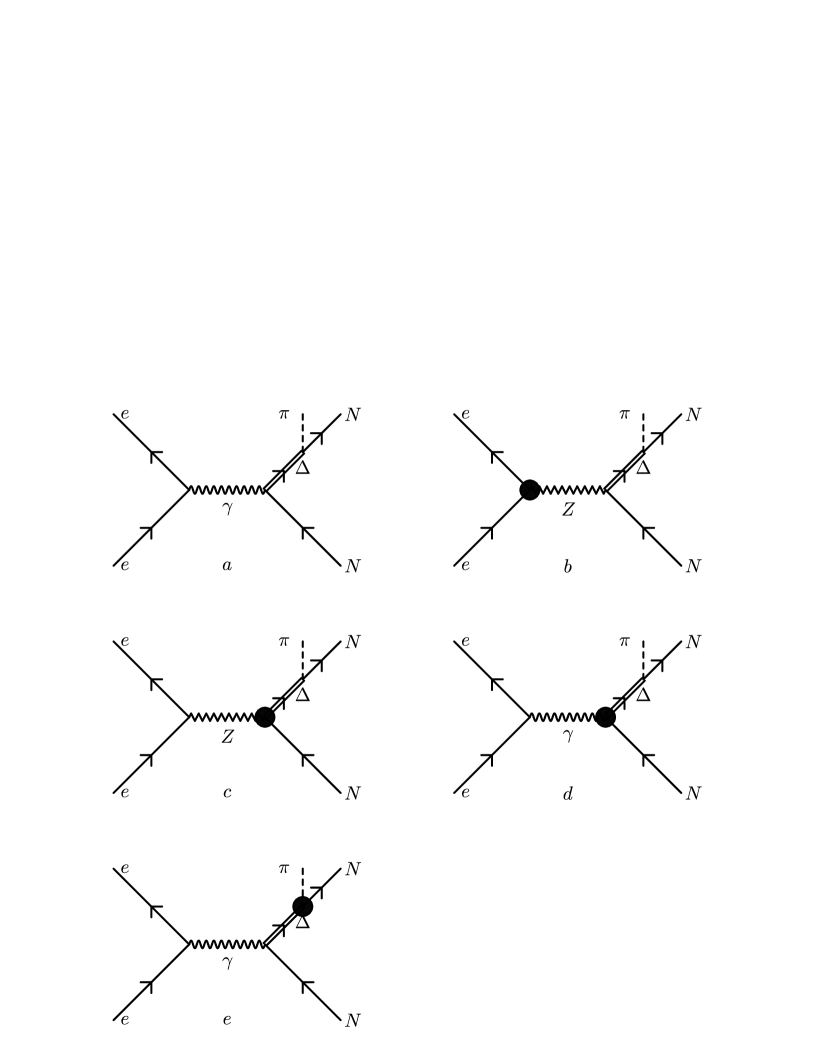
FIG. 1.: Feynman diagrams describing resonant pion electroproduction. The dark circle indicates a parity violating coupling. Fig. 1d gives transition anapole and Siegert’s term contributions. Fig. 1e leads to the PV d-wave $\pi N\Delta$ contribution.

FIG. 2.: Meson-nucleon intermediate state contributions to the $N\to\Delta$ transition anapole and Siegert couplings $a_{\Delta}$ and $d_{\Delta}$, respectively. The shaded circle denotes the PV vertex. The single solid, double solid, dashed, and curly lines correspond to the $N$, $\Delta$, $\pi$, and $\gamma$, respectively.

FIG. 3.: Same is Fig. 2 but with $\Delta$-$\pi$ intermediate states.

FIG. 4.: Same as Fig. 2 but involving insertions of the baryon magnetic moment operator, denoted by the cross.

FIG. 5.: Same as Fig. 2 but with PV electromagnetic insertions, denoted by the overlapping cross and shaded circle.

FIG. 6.: Vector meson contribution to $a_{\Delta}$. Shaded circle indicates PV hadronic coupling. The wavy line is the photon field which transforms into the vector mesons denoted by the double line.

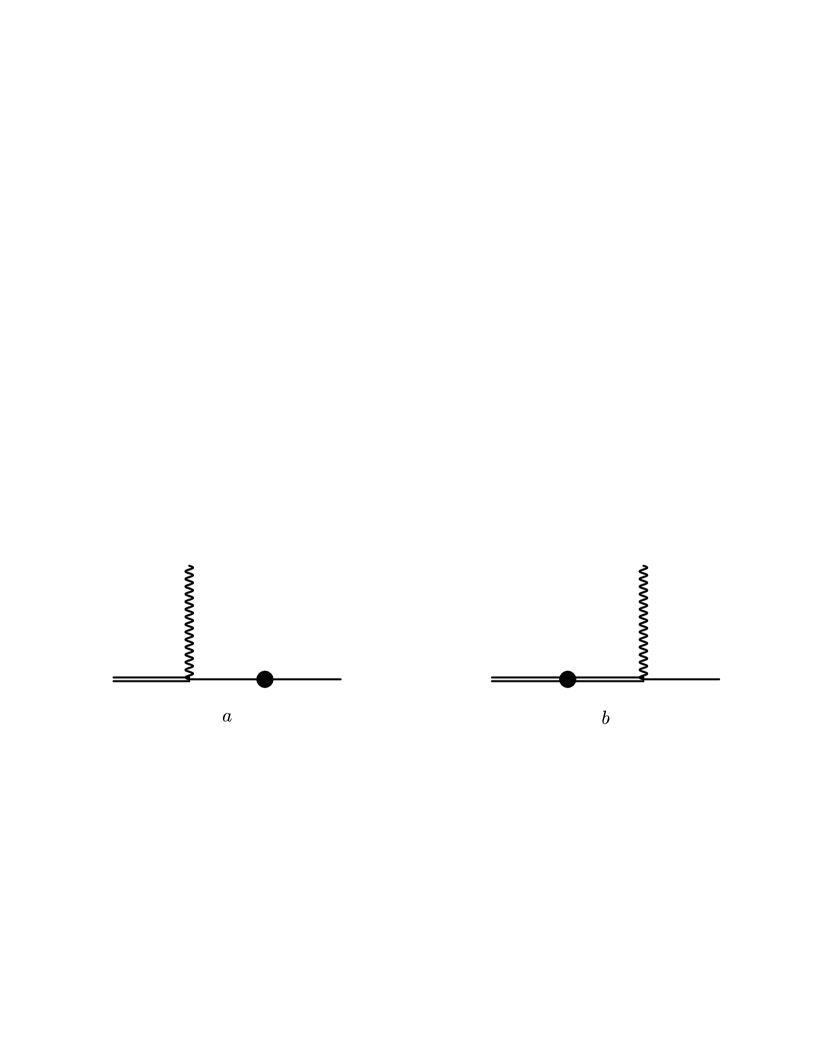
FIG. 7.: Resonance saturation contributions to $d_{\Delta}^{CT}$, where shaded circle denotes PV transition matrix element.

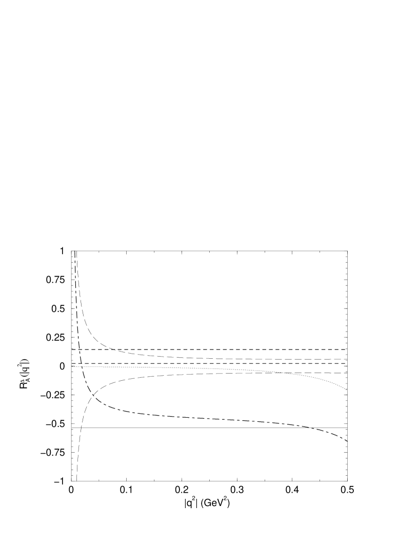
FIG. 8.: Contributions to the electroweak radiative correction $R_{A}^{\Delta}$ at beam energy $0.424$ GeV. The short-dashed lines show the upper and lower bounds of the reasonable range for anapole contribution. The solid line is the one-quark contribution. The upper (lower) long-dashed line is the Siegert term with $d_{\Delta}=25g_{\pi}\ (-25g_{\pi})$. The dotted line is the d-wave contribution.

FIG. 9.: Ratio of asymmetry components $r_{i}=A^{i}_{LR}/A^{NC}_{LRtot}$, where $A^{NC}_{LRtot}$ denotes the total neutral current contribution. The dotted line gives the Siegert contribution; the long-dashed line is for the PV d-wave; the short dashed lines give our “reasonable range” for the anapole effect; and the solid line is for axial vector neutral current contribution. All the other parameters are the same as in Figure 8.

FIG. 10.: Same as Fig. 9 but omitting the anapole and PV d-wave curves and showing Siegert contribution for several values of the coupling $d_{\Delta}$. The dotted, dashed and dashed-dotted lines are for $d_{\Delta}=1g_{\pi},\ 25g_{\pi}$ and $100g_{\pi}$ respectively. The solid line is for the axial vector neutral current contribution. All the other parameters are the same as in Figure 9.

FIG. 11.: Asymmetry components as a function of $|q^{2}|$ and beam energy $0.424$ GeV. Except for $d_{\Delta}$, all the parameters are taken from the central values of the table (VI). The bold long-dashed (dashed) line is for $A_{LR}(\Delta_{(1)}^{\pi})$ ($A_{LR}(\Delta_{(2)}^{\pi})$). The solid, dashed-dotted, dotted and dashed lines are for $A_{LR}(\Delta_{(3)}^{\pi})$ at $d_{\Delta}=0,25,75$ and $100\ g_{\pi}$.

FIG. 12.: Total asymmetry at small $|q^{2}|$ for several $d_{\Delta}$. The couplings are at central values of table (VI). The lines for $d_{\Delta}=0,25,75$ and $100\ g_{\pi}$ are the solid, dashed, dashed-dotted, dotted and long-dashed line.

FIG. 13.: Loop corrections to the PV d-wave $\pi N\Delta$ vertex involving nucleon intermediate states.

FIG. 14.: Same as Fig. 13 but with $\Delta$ intermediate states.

REFERENCES

[1]R. Dashen, E. Jenkins and A. Manohar, Phys. Rev. D 49,
4713 (1994); D 51, 3697 (1995).
[2]D. R. T. Jones and S. T. Petcov, Phys. Lett. B 91, 137
(1980).
[3]S. L. Adler, Ann. Phys. 50, 89 (1968); Phys. Rev. D 12, 2644
(1975).
[4]P. A. Schreiner and F. von Hippel, Nucl. Phys. B 38, 333
(1973).
[5]N. C. Mukhopadhyay et al., Nucl. Phys. A 633, 481 (1998).
[6]D. Leinweber, T. Draper, and R.M. Woloshyn, Phys. Rev. D 46,
3067 (1992).
[7]T. R. Hemmert, B.R. Holstein, and N.C. Mukhopadhyay, Phys.
Rev. D 51, 158 (1995).
[8]G0 Collaboration, JLAB # E97-104, S.P. Wells and
N. Simicevic, spokespersons.
[9]Shi-Lin Zhu, S. Puglia, M. J. Ramsey-Musolf, and B. Holstein,
Phys. Rev. D 62, 033008 (2000).
[10]M. J. Musolf and B. R. Holstein, Phys. Lett. B 242, 461
(1990).
[11]M. J. Musolf and B. R. Holstein, Phys. Rev. D 43, 2956 (1991).
[12]R. Hasty et al., Science 290, 2117 (2000).
[13]J.-W. Chen and X. Ji, Phys. Rev. Lett. 86, 4239 (2001).
[14]Shi-lin Zhu, C. Maekawa, B.R. Holstein, and M.J.
Ramsey-Musolf, hep-ph/0106216.
[15]A.J.F. Siegert, Phys. Rev. 52, 787 (1937).
[16]J.L. Friar and S. Fallieros, Phys. Rev. C 29, 1654 (1984).
[17]W.C. Haxton, E.M. Henley, and M.J. Musolf, Phys. Rev.
Lett. 63, 949 (1989).
[18] The operator in Eq. (5) was independently
written down by the authors of Ref. [13].
[19]Y. Hara, Phys. Rev. Lett. 12, 378 (1964).
[20]A. Le Yaouanc et al., Nucl. Phys. B 149, 321 (1979);
M. B. Gavela et al, Phys. Lett. B 101, 417 (1981).
[21]
B. Borasoy and B. R. Holstein, Phys. Rev. D 59, 054019 (1999).
[22] M.J. Musolf et al., Phys. Reports 239, 1 (1994).
[23] M. J. Musolf and T. W. Donnelly, Nucl. Phys. A546
(1992) 509; ibid. A550 (1992) 564(E).
[24]Particle Data Group, C. Caso et al., Eur. Phys. J. C 3, 55
(1998).
[25]H.-W. Hammer and D. Drechsel, Z. Phys. A 353, 321 (1995).
[26]B. Desplanques, J. F. Donoghue and B. R. Holstein, Ann. Phys.
124, 449 (1980).
[27] Shi-lin Zhu, S.J. Puglia, B.R. Holstein, and M.J.
Ramsey-Musolf, hep-ph/0012253 (2000), Phys. Rev. C (in press).
[28]T. R. Hemmert, B. R. Holstein and J. Kambor, J. Phys. G 24,
1831 (1998).
[33]A. Manohar and H. Georgi, Nucl. Phys. B 234, 189 (1984).
[34]G. Ecker, J. Gasser, A. Pich and E. de Rafael, Nucl.
Phys. B 321, 311 (1989).
[35]G. B. Feldman et al., Phys. Rev. C 43, 863 (1991).
[36]R. Balzer et al., Phys. Rev. C 30, 1409 (1984).
[37] B. Desplanques, Nucl. Phys. A 335, 147 (1980).
[38]E. G. Adelberger and W. C. Haxton, Ann. Rev. Nucl. Part.
Sci. 35, 501 (1985).
[39]W. Haeberli and B.R. Holstein in Symmetries and
Fundamental
Interactions in Nuclei, W. Haxton and E. Henley, Eds., World Scientific,
Singapore
(1995) p. 17-66.
[40] G. Höhler et al., Nucl. Phys. B114, 505
(1976).
[41]KTeV Collaboration, A. Alvavi-Harati et al.,
Phys. Rev. Lett. 86, 3239 (2001).
[42]J. J. Sakurai, Currents and mesons, the University of
Chicago Press, 1969.
[43] D.T. Spayde et al., Phys. Rev. Lett. 84, 1106
(2000);
B.A. Mueller et al., Phys. Rev. Lett. 78, 3824 (1997); R. Hasty et al.,
Science 290, 2117 (2000); K.A. Aniol et al., Phys. Rev. Lett. 82, 1096
(1999);
K.A. Aniol et al., nucl-ex/00060002; MIT-Bates experiment 00-04, T.
Ito,
spokesperson; Jefferson Lab experiment 99-115, K. Kumar and D. Lhuillier,
spokespersons; Jefferson Lab experiment 00-114, D. Armstrong, spokesperson;
Jefferson Lab experiment 91-004, E. Beise, spokesperson; Mainz experiment
PVA4,
D. von Harrach, spokesperson, F. Maas, contact person; Jefferson Lab
experiment
00-006, D. Beck, spokesperson.
[44] Jefferson Lab experiment 00-003, R. Michaels, P. Souder, and
R. Urciuoli, spokespersons.
[45] W.M. Snow et al., Nucl. Inst. Meth. A440, 729
(2000);
Jefferson Lab Letter of Intent 00-002, W. van Oers and B. Wojtsekhowski,
spokespersons; J.F. Cavagnac, B. Vignon, and R. Wilson, Phys. Lett. B67, 148
(1997);
D.M. Markhoff, Ph.D. Thesis, University of Washington (1997).
[46]H.N. Brown et al., Phys. Rev. Lett. 86, 2227 (2001).
[47]B. J. Bjorken and S. Drell, Relativistic Quantum Fields,
McGraw-Hill, New York, 1965.