Precision determination of $|V_{ub}|$ from inclusive decays

Abstract

We propose determining $|V_{ub}|$ from inclusive semileptonic $B$ decay using combined cuts on the leptonic and hadronic invariant masses to eliminate the $b\to c$ background. Compared to a pure dilepton invariant mass cut, the uncertainty from unknown order $\Lambda_{\rm QCD}^{3}/m_{b}^{3}$ terms in the OPE is significantly reduced and the fraction of $b\to u$ events is roughly doubled. Compared to a pure hadronic invariant mass cut, the uncertainty from the unknown light-cone distribution function of the $b$ quark is significantly reduced. We find that $|V_{ub}|$ can be determined with theoretical uncertainty at the 5–10% level.

I Introduction

The magnitude of the Cabibbo-Kobayashi-Maskawa matrix element $V_{ub}$ is an important ingredient in overconstraining the unitarity triangle by measuring its sides and angles. Inclusive semileptonic $b\to u$ decay provides the theoretically cleanest method of measuring $|V_{ub}|$ at present, since it can be calculated model independently using an operator product expansion (OPE) as a double expansion in powers of $\Lambda_{\rm QCD}/m_{b}$ and $\alpha_{s}(m_{b})$ [1]. However, the phase space cuts which are required to eliminate the overwhelming background from $b\to c$ decay typically cause the standard OPE to fail. This is the case both for the cut on the charged lepton energy, $E_{\ell}>(m_{B}^{2}-m_{D}^{2})/2m_{B}$ [2], as well as for the cut on the hadronic invariant mass, $m_{X}<m_{D}$ [3, 4, 5]. In both of these cases, the standard OPE becomes, in the restricted region, an expansion in powers of $\Lambda_{\rm QCD}m_{b}/m_{c}^{2}$, which is of order unity.

Recently we showed that a cut on the dilepton invariant mass can be used to reject the background from $b\to c$ decay [6, 7], while still allowing an expansion in local operators. Imposing a cut $q^{2}>(m_{B}-m_{D})^{2}$ (where $q$ is the four-momentum of the virtual $W$) removes the $b\to c$ background while leaving the OPE valid. This approach has the advantage of being model independent, but is only sensitive to $\sim 20\%$ of the rate, as opposed to $\sim 80\%$ for a $m_{X}<m_{D}$ hadronic invariant mass cut. Besides the sensitivity to $m_{b}$, the main uncertainty in the analysis using a pure $m_{X}$ cut comes from uncalculable corrections, formally of order $\Lambda_{\rm QCD}/m_{b}$, to the $b$ quark light-cone distribution function, while in the case of the pure $q^{2}$ cut from the order $(\Lambda_{\rm QCD}/m_{b})^{3}$ corrections in the OPE, the importance of which was recently stressed [8]. In addition, because of finite detector resolution, the actual experimental cut on $q^{2}$ may be larger than the optimal value of $(m_{B}-m_{D})^{2}$, and the theoretical error in $|V_{ub}|$ grows rapidly as $q^{2}$ is raised.

In this paper we propose to improve on both methods by combining cuts on the leptonic and hadronic invariant mass. Varying the $q^{2}$ cut in the presence of a cut on $m_{X}$ allows one to interpolate continuously between the limits of a pure $q^{2}$ cut and a pure $m_{X}$ cut. We examine how a combined cut on $m_{X}$ and $q^{2}$ can minimize the overall uncertainty. This also allows a precision determination of $|V_{ub}|$ to be obtained with cuts which are away from the threshold for $B\to X_{c}\ell\bar{\nu}_{\ell}$, an important criterion for realistic detector resolution.

In Sec. II we discuss the regions of phase space and explain which ones are accessible within the standard OPE. In Sec. III we present the decay rate with a combined cut on the leptonic and hadronic invariant mass to order $\Lambda_{\rm QCD}^{2}/m_{b}^{2}$ in the OPE and to order $\alpha_{s}^{2}\beta_{0}$ in the perturbative expansion, including a detailed investigation of the theoretical uncertainties. Our results are summarized in Sec. IV.

II Kinematics

The Dalitz plot for $b\to u$ semileptonic decay in the $q^{2}-m_{X}^{2}$ plane is shown in Fig. 1. While the region of phase space contained by the $q^{2}>(m_{B}-m_{D})^{2}$ cut corresponds to a subset of the region $m_{X}<m_{D}$, the theoretical prediction for the former region is better behaved [6]. This may seem counterintuitive, since uncertainties for inclusive observables usually decrease the more inclusive the quantity is. The present situation occurs because the OPE breaks down when the kinematics is restricted to large energy and low invariant mass final states, for which $m_{X}^{2}/E_{X}\sim\Lambda_{\rm QCD}$. As it is explained below, this kinematics dominates the lower left corner of the Dalitz plot in Fig. 1, and that is why the OPE is better behaved in the restricted region determined by the $q^{2}$ cut.

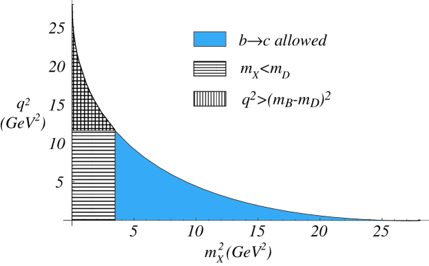
FIG. 1.: The Dalitz plot for $b\to u$ semileptonic decay, indicating the regions corresponding to $b\to c$ decay (shaded), the lepton invariant mass cut $q^{2}>(m_{B}-m_{D})^{2}$ (vertically striped), and the hadron invariant mass cut $m_{X}<m_{D}$ (horizontally striped).

More precisely, there are three distinct regions of phase space, in which the behavior of the OPE is qualitatively different. Over most of the Dalitz plot, the kinematics typically satisfies

$$m_{X}\gg\Lambda_{\rm QCD}\,,\qquad m_{X}^{2}/E_{X}\gg\Lambda_{\rm QCD}\,,$$ (1)

and the inclusive rate may be expanded in powers of $\Lambda_{\rm QCD}/m_{b}$ via the OPE. The leading order term is the $b$ quark decay result, and the higher order terms are parametrized by matrix elements of local operators. This is the simplest region theoretically, since reliable predictions can be made knowing only the first few matrix elements, which may be determined from other processes. The situation is more complicated in the “shape function” region, which is dominated by low invariant mass and high energy final states

$$m_{X}\gg\Lambda_{\rm QCD}\,,\qquad m_{X}^{2}/E_{X}\sim O(\Lambda_{\rm QCD})\,.$$ (2)

In this region, a class of contributions proportional to powers of $\Lambda_{\rm QCD}E_{X}/m_{X}^{2}$ must be resummed to all orders. The OPE is replaced by a twist expansion, in which the leading term depends on the light-cone distribution function of the $b$ quark in the $B$ meson. Since this is a nonperturbative function, the leading order prediction is model dependent, unless the distribution function is measured from another process. Even if this light cone distribution function is extracted from the photon energy spectrum in $B\to X_{s}\gamma$ [9, 10], the unknown higher order corrections are only suppressed by $\Lambda_{\rm QCD}/m_{b}$. Finally, in the resonance regime,

$$m_{X}\sim O(\Lambda_{\rm QCD})\,,$$ (3)

the final state is dominated by a few exclusive resonances and the inclusive description breaks down. In this case neither the local OPE nor the twist expansion is applicable.

Which of these situations applies to the kinematic regions $m_{X}<m_{D}$ and $q^{2}>(m_{B}-m_{D})^{2}$ depends on the relative sizes of $m_{b}$, $m_{c}$ and $\Lambda_{\rm QCD}$. It seems most reasonable to treat

$$\Lambda_{\rm QCD}\,m_{B}\sim O(m_{D}^{2})\,,$$ (4)

since neither side is much larger than the other. Cutting only on the hadronic invariant mass (or on $E_{\ell}$), the hadronic energy can extend all the way to order $m_{B}$,

$$m_{X}\sim m_{D}\,,\qquad E_{X}\sim m_{B}\,,$$ (5)

and so $m_{X}^{2}/E_{X}$ is typically of order $\Lambda_{\rm QCD}$. By contrast, the cut on $q^{2}$ implies

$$m_{X}\sim m_{D}\,,\qquad E_{X}=\frac{m_{B}^{2}-q^{2}+m_{X}^{2}}{2m_{B}}\sim m_{D}\,,$$ (6)

and so typically $m_{X}^{2}/E_{X}\sim m_{D}$. Viewing $m_{D}\gg\Lambda_{\rm QCD}$, both regions are parametrically far from the resonance regime (3). However, the $m_{X}<m_{D}$ (or $E_{\ell}>(m_{B}^{2}-m_{D}^{2})/2m_{B}$) region is in the shape function regime [see, Eq. (2)], and thus sensitive to the light-cone distribution function. In contrast, the region $q^{2}>(m_{B}-m_{D})^{2}$ is parametrically far from both the resonance and shape function regimes.

Thus, the cut on $q^{2}$ eliminates the region where the structure function is important, making the calculation of the partially integrated rate possible in an expansion of local operators. However, from Eq. (6), imposing a cut $q^{2}<q_{\rm cut}^{2}=(m_{B}-m_{X})^{2}$ results in the effective expansion parameter for the OPE being

$${\Lambda_{\rm QCD}E_{X}\over m_{X}^{2}}\sim{\Lambda_{\rm QCD}\over m_{X}}\sim{m_{b}\Lambda_{\rm QCD}\over m_{b}^{2}-q_{\rm cut}^{2}},$$ (7)

and so the convergence of the OPE gets worse as $q_{\rm cut}^{2}$ is raised. For $q_{\rm cut}^{2}=(m_{B}-m_{D})^{2}\simeq(m_{b}-m_{c})^{2}$, the OPE is an expansion in $\Lambda_{\rm QCD}/m_{c}$ [11]. For a very high cut on $q^{2}$ (say, above $\sim 18\,\mbox{GeV}^{2}$), the phase space is restricted to the resonance region, causing a breakdown of the OPE.

For the pure $q^{2}$ cut, the largest uncertainties originate from the $b$ quark mass and the unknown contributions of dimension-six operators, suppressed by $[m_{b}\Lambda_{\rm QCD}/(m_{b}^{2}-q_{\rm cut}^{2})]^{3}$. In this paper we propose that the uncertainties can be reduced considerably by lowering the cut on $q^{2}$ below $(m_{B}-m_{D})^{2}$, and using a simultaneous cut on $m_{X}$ to reject $b\to c$ events. It is obvious that lowering $q_{\rm cut}^{2}$ all the way to zero would result in the rate with just the cut on $m_{X}$, which depends strongly on the light-cone distribution function. Thus lowering $q_{\rm cut}^{2}$ in the presence of a fixed cut on $m_{X}$ increases the uncertainty from the structure function, while decreasing the uncertainty from the matrix elements of the dimension-six operators. The optimal combination of the two cuts is somewhere in between the pure $q^{2}$ and pure $m_{X}$ cuts. In the rest of this paper we calculate the the partially integrated rate and its uncertainty in the presence of cuts on $q^{2}$ and $m_{X}$.

III Combined Cuts

The integrated rate with a lower cut $q_{\rm cut}^{2}$ on $q^{2}$ and an upper cut $m_{\rm cut}$ on $m_{X}$ may be written as

$$\int_{\hat{q}_{\rm cut}^{2}}^{1}{\rm d}\hat{q}^{2}\int_{0}^{\hat{s}_{0}}{\rm d}\hat{s}\,{{\rm d}\Gamma\over{\rm d}\hat{q}^{2}{\rm d}\hat{s}}\equiv{G_{F}^{2}|V_{ub}|^{2}\,(4.7\,{\rm GeV})^{5}\over 192\pi^{3}}\;G(q_{\rm cut}^{2},m_{\rm cut})\,,$$ (8)

where where $\hat{q}=q/m_{b}$, $\hat{s}=(v-\hat{q})^{2}$ is the rescaled partonic invariant mass, $v$ is the four-velocity of the decaying $B$ meson, and

$$\hat{s}_{0}=\cases{\displaystyle\left(1-\sqrt{\hat{q}^{2}}\right)^{2}&for~{} $m_{\rm cut}>m_{B}-m_{b}\,\sqrt{\hat{q}^{2}}$\,,\vspace*{6pt}\cr\displaystyle 0&for~{} $m_{\rm cut}^{2}<(m_{B}-m_{b}\,\hat{q}^{2})\,(m_{B}-m_{b})$\,,\vspace*{6pt}\cr\displaystyle\frac{m_{\rm cut}^{2}}{m_{B}m_{b}}+\left(\frac{m_{B}}{m_{b}}-1\right)\left(\frac{m_{b}}{m_{B}}\,\hat{q}^{2}-1\right)&otherwise\,.\cr}$$ (9)

The hadronic invariant mass $m_{X}$ is related to $\hat{q}^{2}$ and $\hat{s}$ by

$$m_{X}^{2}=\hat{s}\,m_{B}m_{b}+(m_{B}-m_{b})(m_{B}-\hat{q}^{2}m_{b})\,.$$ (10)

$G(q_{\rm cut}^{2},m_{\rm cut})$ is the ratio of the semileptonic $b\to u$ width with cuts on $q^{2}$ and $m_{X}$ to the full width at tree level with $m_{b}=4.7\,{\rm GeV}$. The fraction of semileptonic $b\to u$ events included in the cut rate is $\simeq 1.21\,G(q_{\rm cut}^{2},m_{\rm cut})$. Note that the $m_{b}^{5}$ prefactor, a large source of uncertainty, is included in $G(q_{\rm cut}^{2},m_{\rm cut})$. The theoretical uncertainty in the extraction of $|V_{ub}|$ is therefore half the uncertainty in the prediction for $G(q_{\rm cut}^{2},m_{\rm cut})$.

A Standard OPE

For $q^{2}>(m_{B}-m_{\rm cut})^{2}$, the effects of the structure function are parametrically suppressed, and correspond to including a class of subleading higher order terms in the OPE. In this region the standard OPE is appropriate, and the double differential decay rate is given by

$${1\over\Gamma_{0}}\,{{\rm d}\Gamma\over{\rm d}\hat{q}^{2}{\rm d}\hat{s}} = \delta(\hat{s})\left[\bigg{(}1+{\lambda_{1}\over 2m_{b}^{2}}\bigg{)}\,2\,(1-\hat{q}^{2})^{2}\,(1+2\hat{q}^{2})+{\lambda_{2}\over m_{b}^{2}}\,(3-45\hat{q}^{4}+30\hat{q}^{6})\right]$$ (12)

$${}+{\alpha_{s}(m_{b})\over\pi}\,X(\hat{q}^{2},\hat{s})+\bigg{(}{\alpha_{s}(m_{b})\over\pi}\bigg{)}^{2}\,\beta_{0}\,Y(\hat{q}^{2},\hat{s})+\ldots\,,$$

where $\beta_{0}=11-2n_{f}/3$ and

$$\Gamma_{0}={G_{F}^{2}\,|V_{ub}|^{2}\,m_{b}^{5}\over 192\,\pi^{3}}$$ (13)

is the tree level $b\to u\ell\bar{\nu}$ decay rate. The matrix element $\lambda_{2}$ is known from the $B^{*}-B$ mass splitting, $\lambda_{2}=0.12\,{\rm GeV}^{2}$ (the uncertainty in this relation is included in the $O(1/m_{b}^{3})$ terms). $\lambda_{1}$ is much less well known but, as is clear from (12), the rate is very insensitive to it. The ellipses in Eq. (12) denote order $\alpha_{s}^{2}$ terms not enhanced by $\beta_{0}$, order $(\Lambda_{\rm QCD}/m_{b})^{2}$ terms proportional to derivatives of $\delta(\hat{s})$, and higher order terms in both series. The function $X(\hat{q}^{2},\hat{s})$ can be obtained from the triple differential rate given in [12], and the function $Y(\hat{q}^{2},\hat{s})$ was calculated numerically in [13].

The perturbative contributions to the differential rate in Eq. (12) are finite for $\hat{s}>0$, where only bremsstrahlung diagrams contribute, but singular as $\hat{s}\to 0$. For a fixed value of $m_{X}$, setting $\hat{s}=0$ in Eq. (10) determines how far $q^{2}$ can be lowered without encountering the singularity. Since the singularity is smoothed out by the $b$ quark light-cone distribution function, such low values of $q^{2}$ correspond to the shape function region. Throughout this paper we will therefore stay away from this region by only considering values of $q_{\rm cut}^{2}$ and $m_{\rm cut}$ satisfying

$$q_{\rm cut}^{2}>m_{B}\,m_{b}-m_{\rm cut}^{2}\,\frac{m_{b}}{m_{B}-m_{b}}\,.$$ (14)

This is illustrated in Fig. 2. Note that if $m_{\rm cut}$ is lowered, $q_{\rm cut}^{2}$ must be increased to keep the uncertainty at a roughly constant level. If the difference between the left- and right-hand sides of Eq. (14) is at least few times $\Lambda_{\rm QCD}\,m_{b}$ then we are far from the shape function region, and the OPE is well behaved. In this case the tree level result is not sensitive to the cut on $m_{X}$, and the $\hat{q}^{2}$ spectrum including a hadronic invariant mass cut is given by

$${1\over\Gamma_{0}}\,{{\rm d}\Gamma_{c}(m_{\rm cut})\over{\rm d}\hat{q}^{2}} = \bigg{(}1+{\lambda_{1}\over 2m_{b}^{2}}\bigg{)}\,2\,(1-\hat{q}^{2})^{2}\,(1+2\hat{q}^{2})+{\lambda_{2}\over m_{b}^{2}}\,(3-45\hat{q}^{4}+30\hat{q}^{6})$$ (16)

$${}+{\alpha_{s}(m_{b})\over\pi}\,\tilde{X}(\hat{q}^{2},m_{\rm cut})+\bigg{(}{\alpha_{s}(m_{b})\over\pi}\bigg{)}^{2}\,\beta_{0}\,\tilde{Y}(\hat{q}^{2},m_{\rm cut})+\ldots\,,$$

where the functions $\tilde{X}(\hat{q}^{2},m_{\rm cut})$ and $\tilde{Y}(\hat{q}^{2},m_{\rm cut})$ are given in the Appendix.

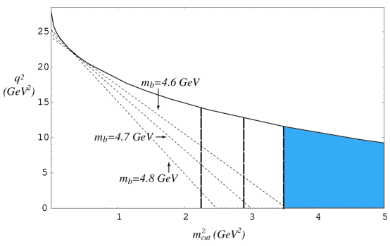
FIG. 2.: The thin dashed lines show the location of the perturbative singularity of ${\rm d}\Gamma_{c}(m_{\rm cut})/{\rm d}q^{2}$, given by Eq. (14), for $m_{b}=4.6,\ 4.7$ and $4.8\,{\rm GeV}$. The thick dashed lines correspond to $m_{\rm cut}=1.5,\ 1.7$ and $1.86\,{\rm GeV}$. The intersection of the thick and thin dashed lines give qualitatively, for a given value of $m_{\rm cut}$, the value of $q_{\rm cut}^{2}$ below which the effects of the distribution function become large.

The differential decay rate in Eq. (16) is given in terms of the pole mass, $m_{b}^{\rm pole}$. It is well-known that use of the pole mass introduces spurious poor behavior of the perturbation series. Although this cancels in relations between physical observables, it is simplest to avoid it from the start by using a better mass definition. There are a number of possibilities; here we choose the $1S$ mass, which is defined as one half of the $\Upsilon(1S)$ mass in perturbation theory. To the order we are working, it is related to the pole mass by

$$m_{b}^{1S}=m_{b}^{\rm pole}\left\{1-\frac{\left(C_{F}\,\alpha_{s}\right)^{2}}{8}\left[1\epsilon+\frac{\alpha_{s}}{\pi}\,\beta_{0}\left(\ln{\mu\over m_{b}\alpha_{s}C_{F}}+\frac{11}{6}\right)\epsilon_{\rm BLM}^{2}+\ldots\right]\right\},$$ (17)

where powers of $\epsilon\equiv 1$ count the order in the upsilon expansion[14], $C_{F}=4/3$, and $\epsilon^{2}_{\rm BLM}$ denotes the “BLM-enhanced” (by a factor of $\beta_{0}$) $O(\epsilon^{2})$ term. Terms of order $\alpha_{s}^{n}$ in Eq. (16) should be counted as order $\epsilon^{n}$, and terms of the same order in $\epsilon$ in the two series should be combined. The mismatch in orders of $\alpha_{s}$ between (16) and (17) is required for the bad behavior of the two series to cancel[14].

The uncertainties in the OPE prediction for $G(q_{\rm cut}^{2},m_{\rm cut})$ from Eq. (16) come from three separate sources: perturbative uncertainties from the unknown full two-loop result, uncertainties in $b$ quark mass and uncertainties due to unknown matrix elements of local operators at $O(1/m_{b}^{3})$ in the OPE. In the following subsections we will estimate each of these uncertainties separately as the fractional errors on $G(q_{\rm cut}^{2},m_{\rm cut})$. The fractional uncertainty in $|V_{ub}|$ then is one half of the resulting value.

1 Perturbative uncertainties

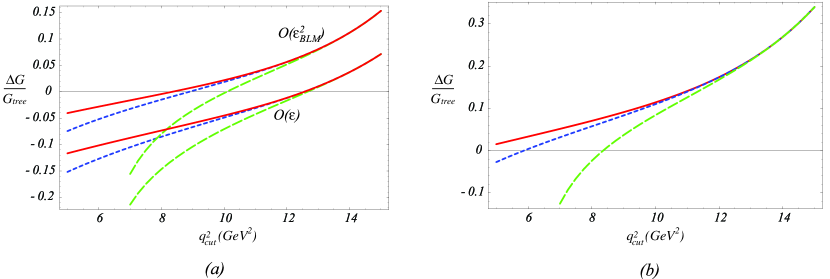
FIG. 3.: (a) The $O(\epsilon)$ and $O(\epsilon^{2}_{\rm BLM})$ contributions to $G(q_{\rm cut}^{2},m_{\rm cut})$ (normalized to the tree level result) for hadronic invariant mass cut $m_{\rm cut}=1.86\,{\rm GeV}$ (solid lines), $1.7\,{\rm GeV}$ (short dashed lines) and $1.5\,{\rm GeV}$ (long dashed lines). (b) Scale variation of the perturbative corrections: The difference between the perturbative corrections to $G(q_{\rm cut}^{2},m_{\rm cut})$, normalized to the tree level result, for $\mu=4.7\,{\rm GeV}$ and $\mu=1.6\,{\rm GeV}$.

The relative sizes of the $O(\epsilon)$ and $O(\epsilon^{2}_{\rm BLM})$ corrections to $G(q_{\rm cut}^{2},m_{\rm cut})$ are plotted in Fig. 3(a), for $\mu=4.7\,{\rm GeV}$. We note that for a given value of $m_{\rm cut}$, the perturbation series is poorly behaved for $q_{\rm cut}^{2}$ both larger and smaller than some optimal range. For large $q_{\rm cut}^{2}$, this behaviour arises because the invariant mass of the final hadronic state is constrained to be small, and so perturbation theory breaks down. For lower values of $q_{\rm cut}^{2}$, the perturbative singularity discussed in the previous section is being approached, and there are large Sudakov logarithms which blow up. These Sudakov logarithms may in principle be resummed, but since our point in this paper is to avoid the shape function region entirely, we will stay in the intermediate region where ordinary perturbation theory is well behaved.

We may estimate the error in the perturbation series in two ways: (a) as the same size as the last term computed, the order $\epsilon^{2}_{\rm BLM}$ term, or (b) as the change in the perturbation series by varying $\mu$ over some reasonable range. These are illustrated in Fig. 3 (a) and (b), respectively. In Fig. 3(b) we vary the renormalization scale between $\mu=4.7\,{\rm GeV}$ and $\mu=m_{b}/3\sim 1.6\,{\rm GeV}$, and plot the change in the perturbative result (including both $O(\epsilon)$ and $O(\epsilon^{2}_{\rm BLM})$ terms). For a given set of $q_{\rm cut}^{2}$ and $m_{\rm cut}$, we take the perturbative error to be the larger of (a) and (b).

Note that since both the $O(\epsilon)$ and $O(\epsilon^{2}_{\rm BLM})$ terms change sign in the region of interest, this approach may underestimate the error in the perturbative series, particularly near the values of the cuts where the $O(\epsilon^{2}\beta_{0})$ term or the scale variation vanishes. To put the estimate of the perturbative uncertainty on firmer grounds, a complete two-loop calculation of the double differential rate, ${\rm d}\Gamma/{\rm d}q^{2}{\rm d}m_{X}$, is most desirable. This is one of the “simpler” two-loop calculations, since the phase space of the leptons can be factorized.

As an alternate approach, Refs. [11, 15] use the renormalization group to sum leading and subleading logarithms of $m_{b}/(m_{b}-\sqrt{q_{\rm cut}^{2}})$ (for a pure $q^{2}$ cut). However, since this log is not large in the regions we are considering, it is not clear that this improves the result. For example, resumming leading logs of $m_{c}/m_{b}$ for $B\to D^{*}$ semileptonic decay at zero recoil in HQET is known to provide a poor approximation to the full two-loop result, and including the power suppressed $(m_{c}/m_{b})\,\alpha_{s}^{n}\ln^{n}(m_{c}/m_{b})$ terms makes the agreement even worse [16].

2 Uncertainties in the $b$ quark mass

The partially integrated rate depends sensitively on the value of the $b$ quark mass due both to the $m_{b}^{5}$ factor in $G(q_{\rm cut}^{2},m_{\rm cut})$ and the cut on $q^{2}$, as stressed in [11]. Currently, the smallest error of the $1S$ mass is quoted from sum rules [17, 18, 19]. Ref. [19] obtains the value $m_{b}^{1S}=4.69\pm 0.03\,{\rm GeV}$ by fitting an optimized linear combination of moments of the $e^{+}e^{-}\to b\,\bar{b}$ spectrum, which may underestimate the theoretical error [18]; the authors of [18] cite a similar central value with a more conservative error of $\pm 0.08\,{\rm GeV}$. In Fig. 4 we show the effects of a $\pm 80\,{\rm MeV}$ and a $\pm 30\,{\rm MeV}$ uncertainty in $m_{b}^{1S}$ on $G(q_{\rm cut}^{2},m_{\rm cut})$, using the central value $m_{b}^{1S}=4.7\,{\rm GeV}$. The latter error may be achievable using moments of various $B$ decay distributions [20].

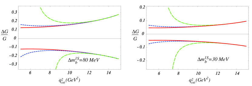
FIG. 4.: The fractional effect of a $\pm 80\,{\rm MeV}$ and $\pm 30\,{\rm MeV}$ uncertainty in $m_{b}^{1S}$ on $G(q_{\rm cut}^{2},m_{\rm cut})$ for $m_{\rm cut}=1.86\,{\rm GeV}$ (solid line), $1.7\,{\rm GeV}$ (short dashed line) and $1.5\,{\rm GeV}$ (long dashed line).

3 ${\cal O}(\Lambda_{\rm QCD}^{3}/m_{b}^{3})$ uncertainties

As discussed in Section II, the convergence of the OPE gets worse as $q_{\rm cut}^{2}$ is raised. Since the contribution from $\lambda_{1}$ in the OPE is small for all values of $q_{\rm cut}^{2}$ (see (16)) and $\lambda_{2}$ is known, the largest uncertainty from unknown nonperturbative terms in the OPE arises at $O(\Lambda_{\rm QCD}^{3}/m_{b}^{3})$ [21]. The effects of these terms were estimated in [6] by varying the values of the corresponding matrix elements over the range expected by dimensional analysis, and determining the corresponding uncertainty in $|V_{ub}|$ as a function of $q_{\rm cut}^{2}$. Since the $b$ quark decay result at tree level is insensitive to the cut on $m_{X}$, as long as $m_{\rm cut}$ is not too low, these results may be immediately taken over to the present analysis. However, the cut on $m_{X}$ allows $q_{\rm cut}^{2}$ to be lowered below $(m_{B}-m_{D})^{2}$, resulting in a significant reduction of the uncertainty, since by (7) it scales as $[m_{b}\Lambda_{\rm QCD}/(m_{b}^{2}-q_{\rm cut}^{2})]^{3}$.

In addition to these corrections, Voloshin [8] has recently stressed the importance of the contribution from weak annihilation (WA) (this uncertainty was included but underestimated in [6]). WA arises at $O(\Lambda_{\rm QCD}^{3}/m_{b}^{3})$ in the OPE, but is enhanced by a factor of $\sim 16\pi^{2}$ because there are only two particles in the final state compared with $b\to u\ell\bar{\nu}_{\ell}$. Because WA contributes only at the endpoint of the $q^{2}$ spectrum, it is independent of $q_{\rm cut}^{2}$ and $m_{\rm cut}$:

$${{\rm d}\Gamma_{WA}\over{\rm d}q^{2}}=-{2G_{F}^{2}|V_{ub}|^{2}m_{b}^{2}\over 3\pi}\delta(q^{2}-m_{b}^{2}){1\over 2m_{B}}\langle B|O^{u}_{V-A}-O^{u}_{S-P}|B\rangle$$ (18)

where

$$O^{q}_{V-A}=\textstyle{1\over 4}\bar{h}_{b}\gamma_{\mu}(1-\gamma_{5})q\bar{q}\gamma^{\mu}(1-\gamma_{5})h_{b},\quad O^{q}_{S-P}=\textstyle{1\over 4}\bar{h}_{b}(1-\gamma_{5})q\bar{q}(1-\gamma_{5})h_{b}.$$ (19)

The matrix element in (18) vanishes for both charged and neutral $B$’s under the factorization hypothesis (in which case it corresponds to pure annihilation, which vanishes by helicity for massless leptons), and so the size of the WA effect depends on the size of factorization violation. Following the discussion in [8] we define the bag constants $B_{i}$ by

$${1\over 2m_{B}}\langle B|O^{u}_{V-A}|B\rangle\equiv{f_{B}^{2}m_{B}\over 8}B_{1},\quad{1\over 2m_{B}}\langle B|O^{u}_{S-P}|B\rangle\equiv{f_{B}^{2}m_{B}\over 8}B_{2}.$$ (20)

Under factorization, $B_{1}=B_{2}=1$ for $B^{\pm}$, and $B_{1}=B_{2}=0$ for $B_{d}$, while Ref. [8] suggests a 10% violation of factorization, $|B_{1}-B_{2}|\sim 0.1$, as being a reasonable estimate. This gives a constant shift to $G(q_{\rm cut}^{2},m_{\rm cut})$ of

$$\delta G(q_{\rm cut}^{2},m_{\rm cut})=16\pi^{2}(B_{2}-B_{1}){f_{B}^{2}\over m_{b}^{2}}\sim 0.03\left({f_{B}\over 0.2\,{\rm GeV}}\right)^{2}\left({B_{2}-B_{1}\over 0.1}\right).$$ (21)

While this corresponds to only a $\sim 3\%$ correction to the total $b\to u\ell\bar{\nu}_{\ell}$ rate, the importance of this correction grows as the cuts reduce the number of events.

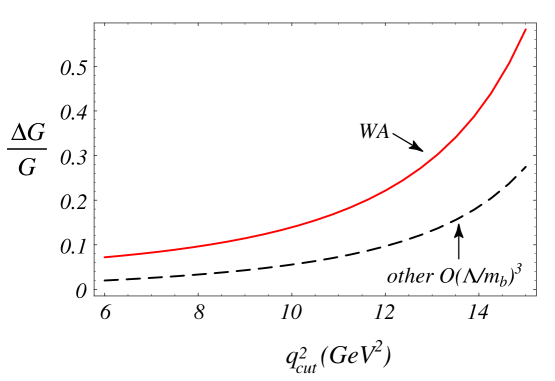
FIG. 5.: Estimate of the uncertainties due to dimension-six terms in the OPE as a function of $q_{\rm cut}^{2}$ from weak annihilation (WA) (solid line) and other operators (dashed line).

The estimated uncertainty from these two classes of $\Lambda_{\rm QCD}^{3}/m_{b}^{3}$ corrections to $G(q_{\rm cut}^{2},m_{\rm cut})$ are plotted in Fig. 5, for $B_{2}-B_{1}=0.1$. Since the uncertainty from WA is roughly a factor of two larger than from the other terms, we use the estimate from WA to determine the theoretical error on $G(q_{\rm cut}^{2},m_{\rm cut})$ from $1/m_{b}^{3}$ effects.

The effects of WA are particularly difficult to estimate because they arise from a small matrix element (factorization violation) multiplying a large coefficient ($16\pi^{2}$), and so further experimental input is required to have confidence in this error estimate. Such spectator effects could be computed using lattice QCD, or could be constrained experimentally from the difference of $|V_{ub}|$ extracted from neutral and charged $B$ decay, or from an experimental measurement of the difference of the semileptonic widths of the $D^{0}$ and $D_{s}$ [8].

B Incorporating the Distribution Function

As $q^{2}$ is lowered below $(m_{B}-m_{\rm cut})^{2}$ the effects of the distribution function become progressively more important, and their size becomes a detailed question depending on the difference between the left- and right-hand sides of Eq. (14). The region where the distribution function becomes significant is correlated with the region where the Sudakov logs from the singularity (14) get large. In the simple model discussed in this section, the impact of the distribution function on the partially integrated rate is indeed roughly constant along the thin dashed lines in Fig. 2, independent of the value of $m_{\rm cut}$.

The $b$ quark light-cone distribution function can be measured from the shape of the photon spectrum in $B\to X_{s}\gamma$, but in the near future such a measurement will have sizable experimental uncertainties. There are also unknown $O(1/m_{b})$ corrections in relating this function to the one relevant for semileptonic $B$ decay (see [24] for a discussion of these terms in the twist expansion). In this paper we restrict ourselves to cuts for which the effect of the distribution function is small, so that its measurement error and the unknown $O(1/m_{b})$ corrections have a small effect in the determination of $|V_{ub}|$.

We still need to estimate the effect of the distribution function to determine how low $q_{\rm cut}^{2}$ may be decreased. Since we restrict ourselves to regions where the effect of the structure function is small, it is sufficient to take them into account at tree level. To leading twist, this is obtained by smearing the $b$ quark decay rate with the distribution function $f(k_{+})$, which amounts to the replacement in Eq. (12),

$$\delta(\hat{s})\to\cases{\displaystyle\int\!{\rm d}k_{+}\,\delta\bigg{(}\hat{s}+\frac{1-\hat{q}^{2}}{m_{b}}\,k_{+}\bigg{)}f(k_{+}),&~{}for $\hat{q}^{2}<(1-\hat{m}_{\rm cut})^{2}$\vspace*{6pt}\cr\displaystyle\delta(\hat{s}),&otherwise.\cr}$$ (22)

(We do not include the distribution function in the region $\hat{q}^{2}>(1-\hat{m}_{\rm cut})^{2}$, since in this region its effects are contained in the $O(\Lambda_{\rm QCD}^{3}/m_{b}^{3})$ terms, which we have already considered.) This corresponds to multiplying the leading order result Eq. (16) in the region $\hat{q}^{2}<(1-\hat{m}_{\rm cut})^{2}$ by a factor

$$A(\hat{q}^{2},m_{\rm cut})=\int_{-s_{0}\frac{m_{b}}{1-\hat{q}^{2}}}^{\Lambda}\!{\rm d}k_{+}\,f(k_{+})\,,$$ (23)

where $s_{0}$ is defined in Eq. (9) and $\Lambda\equiv m_{B}-m_{b}.$ The best way to determine $f(k_{+})$ is from the $B\to X_{s}\gamma$ photon spectrum, which gives at tree level

$$A(\hat{q}^{2},m_{\rm cut})=\frac{1}{2\Gamma^{\gamma}K}\int_{-s_{0}\frac{m_{b}}{1-\hat{q}^{2}}}^{\Lambda}{\rm d}k_{+}\left.{{\rm d}\Gamma^{\gamma}\over{\rm d}E_{\gamma}}\right|_{E_{\gamma}=\frac{m_{b}+k_{+}}{2}}$$ (24)

where $K\sim 1.33$ takes into account contributions from operators other than $O_{7}$ to the photon spectrum [23], and $\Gamma^{\gamma}$ is the contribution of the tree level matrix element of $O_{7}$ to the $B\to X_{s}\gamma$ decay rate. Thus the experimental data on the $B\to X_{s}\gamma$ photon energy spectrum will make the estimate of this source of error small and largely model independent. (Note that the result is modified by large Sudakov logs, which in principle should be resummed, but in the region we are interested these effects are subleading and may be neglected.) Since the dependence of our results on $f(k_{+})$ is weak, even a crude measurement will facilitate a model independent determination of $|V_{ub}|$ from the combined $q^{2}$ and $m_{X}$ cuts with small errors.

In the absence of precise data, we will use the simple model presented in [12] to estimate the effects of the structure function,

$$f(k_{+})={a^{a}\over\Gamma(a)}\,(1-x)^{a-1}\,e^{-a(1-x)}\,,\quad x=\frac{k_{+}}{\Lambda}\,,\quad a=-{3\Lambda^{2}\over\lambda_{1}}\,.$$ (25)

This model is chosen such that its first few moments satisfy the known constraints: the zeroth moment (with respect to $x$) is unity, the first moment vanishes, and the second moment is $\lambda_{1}/3m_{b}^{2}$.

In Fig. 6 we plot in this model the effect of the structure function on $G(q_{\rm cut}^{2},m_{\rm cut})$ as a function of $q_{\rm cut}^{2}$, for three different values of $m_{\rm cut}$. The curves correspond to the parameters $\Lambda=0.57\,{\rm GeV}$ and $\lambda_{1}=-0.2\,{\rm GeV}^{2}$.

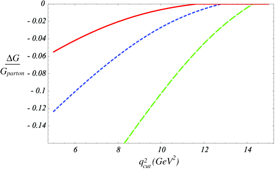
FIG. 6.: The effect of the model structure function (25) on $G(q_{\rm cut}^{2},m_{\rm cut})$ as a function of $q_{\rm cut}^{2}$ for $m_{\rm cut}=1.86\,{\rm GeV}$ (solid line), $1.7\,{\rm GeV}$ (short dashed line) and $1.5\,{\rm GeV}$ (long dashed line).

IV Combined Results

Having considered each uncertainty separately, we now combine them and give the final result for various values of cuts $(q_{\rm cut}^{2},m_{\rm cut})$. In Fig. 7 we plot $G(q_{\rm cut}^{2},m_{\rm cut})$ as a function of $q_{\rm cut}^{2}$ for $m_{\rm cut}=1.5\,{\rm GeV}$, $1.7\,{\rm GeV}$ and $1.86\,{\rm GeV}$. In this figure we choose the values $m_{b}^{1S}=4.7\,{\rm GeV}$, $\lambda_{1}=-0.2\,{\rm GeV}^{2}$ and $\alpha_{s}(m_{b})=0.22$. The combined cut on $q^{2}$ and $m_{X}$ allows a determination of $|V_{ub}|$ from about twice the fraction of events than in the case of the cut on $q^{2}$ alone. The turnaround of the curve for $m_{\rm cut}=1.5\,{\rm GeV}$ signals the breakdown of the perturbation expansion due to the singularity at $\hat{s}=0$, and is not physical.

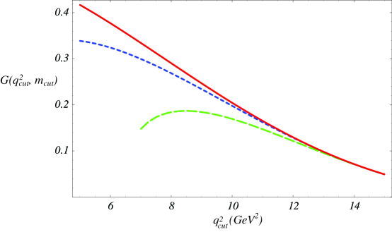
FIG. 7.: $G(q_{\rm cut}^{2},m_{\rm cut})$, which determines the partially integrated rate according to Eq. (8), as a function of the dilepton invariant mass cut $q_{\rm cut}^{2}$, for hadronic invariant mass cut $m_{\rm cut}=1.86\,{\rm GeV}$ (solid line), $1.7\,{\rm GeV}$ (short dashed line) and $1.5\,{\rm GeV}$ (long dashed line).

Cuts on $(q^{2},\,m_{X}^{2})$	$G(q_{\rm cut}^{2},m_{\rm cut})$	$\Delta_{\rm struct}G$	$\Delta_{\rm pert}G$	$\matrix{\Delta_{m_{b}}G\cr{\pm 80/30\,{\rm MeV}}}$	$\Delta_{1/m^{3}}G$	$\Delta G$
Combined cuts
$6\,{\rm GeV}^{2},1.86\,{\rm GeV}$	0.38	$-4\%$	4%	13%/5%	6%	15%/9%
$8\,{\rm GeV}^{2},1.7\,{\rm GeV}$	0.27	$-6\%$	6%	15%/6%	8%	18%/12%
$11\,{\rm GeV}^{2},1.5\,{\rm GeV}$	0.15	$-7\%$	13%	18%/7%	16%	27%/22%
Pure $q^{2}$ cuts
$(m_{B}-m_{D})^{2},m_{D}$	0.14	– –	15%	19%/7%	18%	30%/24%
$(m_{B}-m_{D^{*}})^{2},m_{D^{*}}$	0.17	– –	13%	17%/7%	14%	26%/20%

TABLE I.: $G(q_{\rm cut}^{2},m_{\rm cut})$, as defined in Eq. (8), for several different choices of $(q_{\rm cut}^{2},m_{\rm cut})$, along with the uncertainties. The fraction of $B\to X_{u}\ell\bar{\nu}$ events included by the cuts is $1.21\,G(q_{\rm cut}^{2},m_{\rm cut})$. The two last lines corresponding to pure $q^{2}$ cuts are included for comparison. $\Delta_{\rm struct}G$ gives the fractional effect of the structure function $f(k_{+})$ in the simple model (25); we do not include an uncertainty on this in our error estimate. The overall uncertainty $\Delta G$ is obtained by combining the other uncertainties in quadrature. The two values correspond to $\Delta m_{b}^{1S}=\pm 80\,{\rm MeV}$ and $\pm 30\,{\rm MeV}$. The uncertainty in $|V_{ub}|$ is half of $\Delta G$.

In Table I we use three representative sets of cuts in $q^{2}$ and $m_{X}$ to estimate the overall theoretical uncertainty with which $|V_{ub}|$ can be determined. As throughout this paper, we choose for the cut on the hadronic invariant mass the three values $m_{\rm cut}=(1.5\,{\rm GeV},\,1.7\,{\rm GeV},\,1.86\,{\rm GeV})$. We choose values of $q_{\rm cut}^{2}$ which keep the effects of the distribution function $f(k_{+})$ small (in the simple model discussed in the previous section). Because we anticipate the distribution function will be extracted from the $B\to X_{s}\gamma$ spectrum to the accuracy required, we do not include an uncertainty on $f(k_{+})$ in our overall theoretical uncertainty.

For comparison, we include in Table I the results for a pure $q^{2}$ cut (corresponding to $m_{\rm cut}=m_{B}-\sqrt{q_{\rm cut}^{2}}$), for $q^{2}=(m_{B}-m_{D})^{2}=11.6\,{\rm GeV}^{2}$ and $q^{2}=(m_{B}-m_{D^{*}})^{2}=10.7\,{\rm GeV}^{2}$. We include the second point because $B\to D\ell\bar{\nu}_{\ell}$ is suppressed near zero recoil, and so may be reliably subtracted from the background [7]. These results are consistent with [15], with comparable errors from perturbation theory and $m_{b}$ variation.

A source of uncertainty not explicitly considered in this paper arises from possible quark-hadron duality violation. The size of this is difficult to estimate theoretically, but based on the agreement the values of $|V_{cb}|$ extracted from inclusive and exclusive $B$ decays, we expect it to be smaller than the uncertainties we have considered. Cuts on the phase space may amplify duality violation, but since this technique may be sensitive to almost half of the events, we expect these effects to remain small. In any event, this can be tested experimentally by comparing the extraction of $|V_{ub}|$ with different values of the cuts.

Ultimately, experimental considerations will determine the optimal values of $(q_{\rm cut}^{2},m_{\rm cut})$. An actual analysis will probably be sensitive to the region $q^{2}>q_{\rm cut}^{2}$ and $m_{X}<m_{\rm cut}$ with non-uniform weight. The theoretical errors in such a case will be comparable to our results, as long as the weight function does not vary too rapidly. The formulae presented in the Appendix are sufficient to determine the perturbative relationship of $|V_{ub}|$ and such a measurement. In addition, as explained in [7], due to heavy quark symmetry, the $B\to X_{c}\ell\bar{\nu}$ background near $m_{X}=m_{D}$ may be easier to understand as a function of $q^{2}$ and $m_{X}$ than as a function of $m_{X}$ only. For example, the $D^{**}$ and higher mass states cannot contribute for $q^{2}>8.5\,{\rm GeV}^{2}$, and so the main background is $B\to D^{*}\ell\bar{\nu}$ near zero recoil, which will be precisely measured to determine $|V_{cb}|$.

V Conclusions

In this paper we proposed a precision determination of the magnitude of the CKM matrix element $V_{ub}$ from charmless inclusive semileptonic $B$ decays using combined cuts on the dilepton invariant mass, $q^{2}$, and the hadronic invariant mass, $m_{X}$. This leads to the following general strategy for determining $|V_{ub}|$:

• make the cut on $m_{X}$ as large as possible, keeping the background from $B$ to charm under control

• for a given cut on $m_{X}$, reduce the $q^{2}$ cut as low as possible, keeping the contribution from the $b$ quark structure function, as well as the perturbative uncertainties, small (see Figs. 3 and 6).

We have calculated $G(q_{\rm cut}^{2},m_{\rm cut})$, the partially integrated rate in the presence of cuts on $q^{2}$ and $m_{X}$ (normalized as in Eq. (8)). Our results are summarized for three representative values of the cuts in Table I. The total uncertainty $\Delta G$ is twice the uncertainty in $|V_{ub}|$. The uncertainty from weak annihilation (Fig. 5) may be reduced by comparing results in $B^{\pm}$ and $B^{0}$ decay, or by comparing the semileptonic widths of the $D^{0}$ and $D_{s}$ [8], while the remaining uncertainties could be reduced by an improved determination of the $b$ quark mass and a complete two loop calculation of the doubly differential rate ${\rm d}\Gamma/{\rm d}q^{2}\,{\rm d}m_{X}$.

This method is sensitive to up to $\sim 45\%$ of the $B\to X_{u}\ell\nu$ decays, about twice the fraction of events than in the case of the cut on $q^{2}$ alone. We found that a determination of $|V_{ub}|$ with a theoretical error at the 5–10% level is possible. The combined $(q_{\rm cut}^{2},m_{\rm cut})$ cut also allows this precision to be obtained with cuts which are away from the threshold for $B\to X_{c}\ell\bar{\nu}_{\ell}$, an important criterion for realistic detector resolution. Such a measurement of $|V_{ub}|$ would largely reduce the standard model range of $\sin 2\beta$, and thus allow more sensitive searches for new physics.

The functions $\widetilde{X}(\hat{q}^{2},m_{\rm cut})$ and $\widetilde{Y}(\hat{q}^{2},m_{\rm cut})$

The functions $\tilde{X}(\hat{q}^{2},m_{\rm cut})$ and $\tilde{Y}(\hat{q}^{2},m_{\rm cut})$ in Eq. (16) can be determined from $X(\hat{q}^{2},\hat{s})$ and $Y(\hat{q}^{2},\hat{s})$ defined in Eq. (12) via

$$\tilde{X}(\hat{q}^{2},m_{\rm cut})=\int_{0}^{s_{0}}{\rm d}\hat{s}\,X(\hat{q}^{2},\hat{s})\,,\quad\tilde{Y}(\hat{q}^{2},m_{\rm cut})=\int_{0}^{s_{0}}{\rm d}\hat{s}\,Y(\hat{q}^{2},\hat{s})\,,$$ (26)

where $s_{0}$ is given in (9).

When $m_{\rm cut}>m_{B}-m_{b}\,\sqrt{\hat{q}^{2}}$, the $m_{\rm cut}$ limit does not restrict the ${\rm d}\hat{s}$ integration, and the result is just the value of the single differential $\hat{q}^{2}$ spectrum. The order $\alpha_{s}$ correction to ${\rm d}\Gamma/{\rm d}\hat{q}^{2}$ was computed in Ref. [25],

$$\tilde{X}_{0}(\hat{q}^{2})=-\frac{2}{3}\, \bigg{\{}2(1-\hat{q}^{2})^{2}(1+2\hat{q}^{2})\Big{[}\pi^{2}+2L_{2}(\hat{q}^{2})-2L_{2}(1-\hat{q}^{2})\Big{]}+4\hat{q}^{2}(1-\hat{q}^{2}-2\hat{q}^{4})\ln\hat{q}^{2}$$ (28)

$${}+2(1-\hat{q}^{2})^{2}(5+4\hat{q}^{2})\ln(1-\hat{q}^{2})-(1-\hat{q}^{2})(5+9\hat{q}^{2}-6\hat{q}^{4})\bigg{\}}\,,$$

where $L_{2}(z)=-\int_{0}^{z}{\rm d}t\ln(1-t)/t$ is the dilogarithm. The order $\alpha_{s}^{2}\beta_{0}$ correction to ${\rm d}\Gamma/{\rm d}\hat{q}^{2}$ was computed in Ref. [13] numerically. We find that the following simple function

$$\tilde{Y}_{0}(\hat{q}^{2})\simeq 0.472\,(1-\hat{q}^{2})-32.5\,(1-\hat{q}^{2})^{2}+42.3\,(1-\hat{q}^{2})^{3}-16.0\,(1-\hat{q}^{2})^{4}\,,$$ (29)

gives a very good approximation. It deviates from the exact result by less than $0.01$ for any value of $\hat{q}^{2}$ (while $\int_{0}^{1}\tilde{Y}_{0}(\hat{q}^{2})\,{\rm d}\hat{q}^{2}\simeq-3.22$).

In the second case in Eq. (9), $m_{\rm cut}^{2}<(m_{B}-m_{b}\,\hat{q}^{2})\,(m_{B}-m_{b})$, $m_{\rm cut}$ is too small, and the perturbative calculation is not reliable. As we have discussed, we avoid this region in this paper.

The situation in which neither of the first two cases in Eq. (9) applies is the most interesting for us. We obtain

$$\tilde{X}(\hat{q}^{2},m_{\rm cut}) = \tilde{X}_{0}(\hat{q}^{2})-\frac{4}{3}\,(1-\hat{q}^{2})^{2}(1+2\hat{q}^{2})\Bigg{\{}\frac{\pi^{2}}{3}-\frac{7}{2}\ln(4s_{0})+2(\ln 2)^{2}-(\ln s_{0})^{2}$$ (34)

$$+2\ln T\ln\frac{4s_{0}^{2}}{T}+\left(3+2\ln\frac{T-R+s_{0}}{4T^{2}}\right)\ln(T-R+s_{0})$$

$$-2L_{2}(T)+4L_{2}\bigg{(}\frac{T+R+s_{0}}{2}\bigg{)}-4L_{2}\bigg{(}\frac{T+R+s_{0}}{2T}\bigg{)}\Bigg{\}}$$

$$-\frac{4}{3}\,\Bigg{\{}R(5+7\hat{q}^{2}-8\hat{q}^{4}+s_{0})+s_{0}\,(1+2\hat{q}^{2})\,(4T+s_{0})\ln\frac{T-R+s_{0}}{2\sqrt{s_{0}}}$$

$$-4\hat{q}^{2}(1+\hat{q}^{2})(1-2\hat{q}^{2})\ln\frac{T-R-s_{0}}{\sqrt{\hat{q}^{2}}}+4(1+\hat{q}^{2}-4\hat{q}^{4})\ln(T-R+s_{0})\Bigg{\}}\,,$$

where $R=\sqrt{\hat{q}^{4}+(1-s_{0})^{2}-2\hat{q}^{2}(1+s_{0})}\,$, $T=1-\hat{q}^{2}$, and $s_{0}$ is given in Eq. (9). For the coefficient of the order $\alpha_{s}^{2}\beta_{0}$ correction we find

$$\tilde{Y}(\hat{q}^{2},m_{\rm cut})=\tilde{Y}_{0}(\hat{q}^{2})-\int_{s_{0}}^{\left(1-\sqrt{\hat{q}^{2}}\right)^{2}}{\rm d}s\,\frac{1}{2}\,Z_{2}\bigg{(}s,\frac{1+s-\hat{q}^{2}}{2}\bigg{)}\,,$$ (35)

where

$$Z_{2}(s,e) = \bigg{(}\frac{5}{12}-\frac{1}{4}\ln s\bigg{)}Z_{1}(s,e)-\frac{2}{3s}\,\Bigg{\{}\sqrt{e^{2}-s}\,\Big{[}5e(3-4e)-4s+26es-8s^{2}\Big{]}$$ (39)

$${}+s\,\bigg{[}9-9e-8e^{2}+\frac{8e^{3}}{s}+s+6es-2s^{2}-\frac{3(1-e)}{1-2e+s}\bigg{]}\ln\frac{(e+\sqrt{e^{2}-s})^{2}}{s}$$

$${}+\frac{(2e-s)\sqrt{e^{2}-s}}{1-2e+s}\,\Big{[}12+40e^{2}+5s(5+2s)-4e(11+10s)\Big{]}\ln\frac{(2e-s)^{2}}{s}$$

$${}+(3-4e+2s)(8e^{2}-4es+s^{2})\Bigg{[}L_{2}\Bigg{(}\frac{\sqrt{e^{2}-s}+e-s}{\sqrt{e^{2}-s}-e}\Bigg{)}-L_{2}\Bigg{(}\frac{\sqrt{e^{2}-s}-e+s}{\sqrt{e^{2}-s}+e}\Bigg{)}\Bigg{]}\Bigg{\}}$$

and

$$Z_{1}(s,e) = \frac{16}{3s}\,\sqrt{e^{2}-s}\,[28e^{2}+2s(5+4s)-3e(7+10s)]$$ (41)

$$-\frac{8}{3s}\,(3-4e+2s)(8e^{2}-4es+s^{2})\ln\frac{e-\sqrt{e^{2}-s}}{e+\sqrt{e^{2}-s}}\,.$$

REFERENCES

• [1] J. Chay, H. Georgi and B. Grinstein, Phys. Lett. B247 (1990) 399;
M.A. Shifman and M.B. Voloshin, Sov. J. Nucl. Phys. 41 (1985) 120;
I.I. Bigi et al., Phys. Lett. B293 (1992) 430 [Erratum-ibid. B 297, 430 (1992)];
I.I. Bigi et al., Phys. Rev. Lett. 71 (1993) 496;
A.V. Manohar and M.B. Wise, Phys. Rev. D49 (1994) 1310.
• [2] F. Bartelt et al., CLEO Collaboration, Phys. Rev. Lett. 71 (1993) 4111;
H. Albrecht et al., Argus Collaboration, Phys. Lett. B255 (1991) 297.
• [3] A.F. Falk, Z. Ligeti and M.B. Wise, Phys. Lett. B406 (1997) 225;
I. Bigi, R. D. Dikeman and N. Uraltsev, Eur. Phys. J. C4 (1998) 453 .
• [4] V. Barger et al., Phys. Lett. B251 (1990) 629;
J. Dai, Phys. Lett. B333 (1994) 212.
• [5] R. Barate et al., ALEPH Collaboration, CERN EP/98-067; DELPHI Collaboration, contributed paper to the ICHEP98 Conference (Vancouver), paper 241;
M. Acciarri et al., L3 Collaboration, Phys. Lett. B436 (1998) 174.
• [6] C.W. Bauer, Z. Ligeti and M. Luke, Phys. Lett. B479 (2000) 395.
• [7] C.W. Bauer, Z. Ligeti and M. Luke, hep-ph/0007054.
• [8] M.B. Voloshin, hep-ph/0106040.
• [9] M. Neubert, Phys. Rev. D49 (1994) 4623;
I.I. Bigi et al., Int. J. Mod. Phys. A9 (1994) 2467.
• [10] A.K. Leibovich, I. Low and I.Z. Rothstein, Phys. Rev. D61 (2000) 053006;
Phys. Lett. B486 (2000) 86.
• [11] M. Neubert, JHEP 0007 (2000) 022.
• [12] F. De Fazio and M. Neubert, JHEP 9906 (1999) 017.
• [13] M. Luke, M. Savage, and M.B. Wise, Phys. Lett. B343 (1995) 329.
• [14] A.H. Hoang, Z. Ligeti, and A.V. Manohar, Phys. Rev. Lett. 82 (1999) 277; Phys. Rev. D59 (1999) 074017.
• [15] M. Neubert and T. Becher, hep-ph/0105217.
• [16] M. A. Shifman and M. B. Voloshin, Sov. J. Nucl. Phys.  45, 292 (1987);
H. D. Politzer and M. B. Wise, Phys. Lett. B206, 681 (1988);
A. F. Falk and B. Grinstein, Phys. Lett. B247, 406 (1990);
A. Czarnecki, Phys. Rev. Lett.  76, 4124 (1996).
• [17] M. B. Voloshin, Int. J. Mod. Phys. A10 (1995) 2865;
A. A. Penin and A. A. Pivovarov, Phys. Lett. B435 (1998) 413;
K. Melnikov and A. Yelkhovsky, Phys. Rev. D59 (1999) 114009;
A. H. Hoang, Phys. Rev. D61 (2000) 034005.
• [18] M. Beneke and A. Signer, Phys. Lett. B471 (1999) 233.
• [19] A. H. Hoang, hep-ph/0008102.
• [20] M.B. Voloshin, Phys. Rev. D51 (1995) 4934;
A. Kapustin and Z. Ligeti, Phys. Lett. B355 (1995) 318;
M. Gremm, A. Kapustin, Z. Ligeti, and M.B. Wise, Phys. Rev. Lett. 77 (1996) 20;
A. F. Falk, M. Luke and M. J. Savage, Phys. Rev. D53 (1996) 6316; Phys. Rev. D53 (1996) 2491;
Z. Ligeti, M. Luke, A.V. Manohar and M.B. Wise, Phys. Rev. D60 (1999) 034019.
• [21] C. W. Bauer and C. N. Burrell, Phys. Rev. D62 (2000) 114028;
M. Gremm and A. Kapustin, Phys. Rev. D55 (1997) 6924.
• [22] A. K. Leibovich and I. Z. Rothstein, Phys. Rev. D 61, 074006 (2000);
A. K. Leibovich, I. Low and I. Z. Rothstein, hep-ph/0105066.
• [23] M. Neubert, hep-ph/0104280;
• [24] C. W. Bauer, M. Luke and T. Mannel, hep-ph/0102089.
• [25] M. Jezabek and J. H. Kuhn, Nucl. Phys. B314 (1989) 1.