CP Violation Search in $\tau\rightarrow\pi\pi^{0}\nu_{\tau}$ Decays

Using a sample of 12.2 million $\tau$-lepton pairs produced by $e^{+}e^{-}$ annihilation at $\sqrt{s}\sim 10.6\,$GeV and collected by the CLEO detector, we search for and set limits on $CP$ violation in $\tau$-lepton decays. For each event, we require that both $\tau$-leptons decay via the mode $\tau\rightarrow\pi\pi^{0}\nu$. The search is performed within the context of a multi-Higgs Doublet Model and the imaginary part of the coupling constant parameterizing the non-Standard Model diagram leading to $CP$ violation is constrained to be $-0.046<\Im{(\Lambda})<0.022$ at 90% CL. The novel search technique is of general utility.

1 Introduction

CP violation has long been observed in the kaon system and is expected soon to be seen unambiguously in the $B$-meson system. Searches for CP violation in leptonic decays have been less extensive. Although CP non-conservation in such decays is forbidden in the Standard Model (SM), many extensions $\!{}^{{\bf?}}$ to the SM incorporate it. Multi-Higgs Doublet models (MHDM) $\!{}^{{\bf?}}$${}^{,\,}$$\!{}^{{\bf?}}$ are perhaps the best known. This report describes a novel search technique for $CP$ violation performed with tau decays and for a specific MHDM. The technique is general and no feature of it restricts it to our particular choice of MHDM or final state.

With the CLEO detector, we study $e^{+}e^{-}\rightarrow\tau^{+}\tau^{-}$ events produced at CESR at a center-of-mass energy in the vicinity of the $\Upsilon(4S)$ resonance. We select only those events where each $\tau$ lepton decays in the mode $\tau\rightarrow\pi\pi^{0}\nu_{\tau}$. Interference between the SM process mediated by $W$-boson exchange and a non-SM process mediated by scalar boson exchange could lead to $CP$ violating effects. For each of our events, we construct a $CP$ sensitive variable for which a non-zero value is evidence of $CP$ violation.

CP violation is essentially an interference effect between two (or more) transition amplitudes that have a relative phase difference for both the strong and weak phases. The relative strong phase remains invariant under CP conjugation while the relative weak phase changes sign. Figure 1 shows the basic idea, where $\delta$ and $\phi$ are the relative strong and weak phases, respectively, and the overall transition amplitude $A=A_{1}+A_{2}{\rm e}^{i\phi}{\rm e}^{i\delta}$ for a process leads to its corresponding probability density $P$:

$$\begin{array}[]{rcl}P\propto|A^{2}|&=&(A_{1}+A_{2}{\rm e}^{i\phi}{\rm e}^{i\delta})(A_{1}+A_{2}{\rm e}^{-i\phi}{\rm e}^{-i\delta})\\ &=&A_{1}^{2}+A_{2}^{2}+2A_{1}A_{2}\cos{\phi}\cos{\delta}\\ &&-2A_{1}A_{2}\sin{\delta}\sin{\phi\par}\end{array}$$ (1)

Note that the last term contains the CP-odd factor $\sin{\delta}\sin{\phi}$, which changes sign for the CP-conjugate process, leading to difference in probability densities between a particular transition and its CP conjugate.

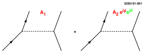
Figure 1: Generic Feynman diagrams for two transition amplitudes that contain CP-even and CP-odd relative phases.

2 Model Choice

To make the foregoing generalities specific and to illustrate the overall search technique, we select a specific MHDM model: a 3 Higgs Doublet model $\!{}^{{\bf?}}$. The relevant Feynman diagrams for this model describing $\tau\rightarrow\pi\pi^{0}\nu_{\tau}$ are shown in figure 2. The SM diagram mediated by a $W$ boson is shown on the left while the non-SM diagram mediated by a charged Higgs is shown on the right. For the SM diagram, the vector form factor that characterizes the final state strong interaction among quarks contains a CP-even phase. The non-SM diagram contains a scalar form factor $f_{s}$, also with a $CP$-even strong phase. The choice of $f_{s}$ is not unique so we consider three choices: $f_{s}=1$, ${f_{s}=\rm BW[a_{0}(980)]}$, and ${f_{s}=\rm BW[a_{0}(1450)]}$. The term BW specifies a Breit-Wigner shape and ${\rm a_{0}}$ indicates a particular intermediate meson resonance.

In this model the second amplitude contains an overall complex coupling $\Lambda$ between the charged Higgs H and the final state, where $\Lambda$ is a function of the $H$ coupling to quarks and leptons. Because $\Lambda$ is complex, it introduces a $CP$ odd phase. Since we have two interfering diagrams with different relative strong and weak phases, CP violation is possible.

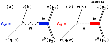
Figure 2: Feynman diagrams for a) the SM amplitude mediated by $W$ exchange and b) the non-SM amplitude mediated by scalar exchange.

3 Choice of Optimal CP-sensitive Variable

In general, we can write the $\tau$ production and decay probability density $P$ as the sum of two terms, one invariant to CP conjugation of the underlying Feynman amplitudes, $P_{even}$, and another that changes under CP conjugation: $P=P_{even}+P_{odd}$. Both $P_{even}$ and $P_{odd}$ are functions of the form factors, the complex coupling $\Lambda$ and kinematic quantities. To search for CP-violation we select the CP-sensitive (i.e. CP odd) observable with the greatest statistical significance and compute it for each event. Such a variable $\!{}^{{\bf?}}$${}^{,\,}$$\!{}^{{\bf?}}$ has been constructed with different searches in mind by other workers:

$$\xi={{\rm P_{odd}\over{\rm P_{even}}}}$$ (2)

$\xi$ is a complicated function, and although it is maximally sensitive to CP violation, has no immediate intuitive appeal. Averaged over the data set, $\langle\xi\rangle\neq 0$ implies CP violation. It can be shown $\!{}^{{\bf?}}$ that

$$\begin{array}[]{rcl}\langle\xi\rangle&=&Im(\Lambda)\int{{\rm P^{2}_{odd}}\over{\rm P_{even}}}\,dLips\\[5.69054pt] &=&c_{1}\lambda+c_{3}\lambda^{3}+c_{5}\lambda^{5}+\ldots,\par\end{array}$$ (3)

where $\lambda\equiv Im(\Lambda)$ and the $c_{i}$ are constants.

The Monte Carlo $\xi$ distribution is shown in figure 3 for the two limits of the model. The left-hand side is for no CP violation and the right-hand side is for the ‘maximal’ case where $Im(\Lambda)$ has a value equal to the SM coupling. The three distributions in each plot correspond to the three choices of the scalar form factor and the structure in each distribution is due to the resonant structure of the vector and scalar form factors. A non-zero value of $\langle\xi\rangle$ for the CP violation case is apparent.

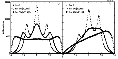
Figure 3: Monte Carlo distributions for the optimal CP-sensitive $\xi$ for the case a) of no CP violation and b) of ‘maximal’ CP violation. See text for discussion.

4 Experimental Details

4.1 Event Selection and Background Estimates

To calculate a value of $\xi$ for each event it is necessary to know the direction of the final state neutrinos to determine the direction of the final state $\tau$-leptons. For those events where each $\tau$ decays semi-hadronically, energy and momentum conservation can be used to determine each $\tau$ direction up to a two-fold ambiguity $\!{}^{{\bf?}}$. Since we have no way of knowing the correct solution for an event, we sum the $\xi$ distributions corresponding to each solution and then average the result to search for an asymmetry. We have checked with Monte Carlo events that this process does not bias our result for the case of no CP violation. For the case of CP violation, we use a special Monte Carlo calibration procedure described below.

We use a data set that corresponds to $13.3\,{\rm fb^{-1}}$ of total integrated luminosity and contains 12.2 million $\tau^{+}\tau^{-}$ pairs produced from $e^{+}e^{-}$ collisions at a center-of-mass energy near or at the $\Upsilon(4S)$. We select events for which each $\tau$ decays via the mode $\tau\rightarrow\pi\pi^{0}\nu$, selected for its large branching fraction ($\simeq 25\%)$) and high selection efficiency (10%). We verify with Monte Carlo events that our selection criteria do not introduce a bias in the $\xi$ distribution.

The major source of background are $\tau$-pair events where one of the $\tau$’s decays to a $\rho\nu$ final state, the other $\tau$ decays to a $\pi\pi^{0}\nu$ final state, and one of the $\pi^{0}$’s is not reconstructed. Using Monte Carlo events, we estimate this contamination level at 5.2% of the selected data. The overall background contamination from $\tau$ decays is estimated at 10%. We estimate that events of the form $e^{-}e^{+}\rightarrow q\bar{q}$ ($q=u,d.c,s$ quarks), $e^{-}e^{+}\rightarrow\Upsilon(4{\rm S})\rightarrow B\bar{B}$, and $e^{-}e^{+}\rightarrow e^{-}e^{+}\gamma\gamma$ contribute a background contamination of less than 0.1%.

4.2 Calibration

From Eq. (3) we see that to lowest order $\langle\xi\rangle=c_{1}\lambda$. To determine or limit $\lambda$, we need to measure $\langle\xi\rangle$ and determine the calibration constant $c_{1}$. This is done in a two step process. First, we determine the range over which $\langle\xi\rangle$ is a linear function of $\lambda$, using Monte Carlo events and assuming perfect detector response. Figure 4 shows $\langle\xi\rangle$ v. $\lambda$ for the three choices of the scalar form factor. After this linear range is determined, we choose 5 values of $\lambda$ within that range, and with full detector simulation compute $\langle\xi\rangle$ for each of the 5 $\lambda$ values. This produces a set of 5 ($\lambda,\langle\xi\rangle$) points to which a straight line is fit. The resulting slope is then $c_{1}$. This entire process is done for each of the 3 scalar form factors.

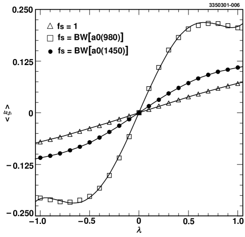
Figure 4: $\langle\xi\rangle$ v. $\lambda$ for each of the three choices for the scalar form factor: a) ${\rm f_{s}=1}$, b) ${\rm f_{s}=BW[a_{0}(980)]}$, and c) ${\rm f_{s}=BW[a_{0}(980)]}$.

5 Results

5.1 Observed $\xi$ Distributions

Using the calibration constant, the $\xi$ distribution for data and Monte Carlo is shown in figure 5 for each of the scalar form factors. The data are squares and the line is SM Monte Carlo. The corresponding measurements for $\langle\xi\rangle$ and the 90% CL limits on $\lambda$, the imaginary part of the non-SM coupling, are shown in table 1.

Table 1: Limits on $Im(\Lambda)$ for various form factors $f_{s}$.

${\rm f_{s}}$	$\langle\xi\rangle\times 10^{-3}$	$Im(\Lambda)\ @\$ 90% CL
${\rm f_{s}=1}$	$-0.8\pm 1.4$	$-0.046<\lambda<.022$
${\rm f_{s}=BW[a_{0}(980)]}$	$-0.1\pm 0.4$	$-0.008<\lambda<.006$
${\rm f_{s}=BW[a_{0}(1450)]}$	$0.1\pm 1.2$	$-0.019<\lambda<.021$

5.2 Systematics

Care is taken to verify that the detector does not create an artificial $\xi$ asymmetry. Systematic effects due to a possible difference between track reconstruction efficiencies for $\pi^{-}$ and $\pi^{+}$ as a function of pion momentum are studied. The momentum distribution for charged pions in the reactions $\tau^{\pm}\rightarrow\pi^{\pm}\pi^{0}\nu_{\tau}$ is plotted in figure 6a. The corresponding ratio of these distributions is shown in figure 6b and is seen to be consistent with 1. Varying the slope of this ratio by $\pm 1\sigma$ leaves $c_{1}$ unchanged but does change $\lambda$ by $\pm 0.003$. We take this as a measure of the systematic error due to differences in the charged pion track reconstruction efficiencies.

Imperfect Monte Carlo simulation of the momentum distributions for the tau decay products can also bias our results. The momentum distributions for charged and neutral pions for both data and Monte Carlo are shown in figure 6c and figure 6d. The agreement is quite good. Varying the slope of these distributions by $\pm 1\sigma$ permits an estimate of the systematic error on $\lambda$ to be made. The effect is negligible ($\sim 10^{-5}$).

A possible asymmetry in the $\xi$ distribution due to background events has been estimated with Monte Carlo and found to be negligible.

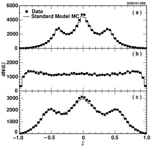
Figure 5: The distribution for the CP-sensitive observable $\xi$ for each of the three choices for the scalar form factor: a) ${\rm f_{s}=1}$, b) ${\rm f_{s}=BW[a_{0}(980)]}$, and c) ${\rm f_{s}=BW[a_{0}(1450)]}$. The squares are the data and the line is SM Monte Carlo.

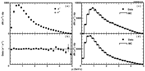
Figure 6: The $\pi^{\pm}$ momentum distributions for data are shown in a) while the ratio is shown in b). The distributions for data and Monte Carlo are shown for charged pions c) and for neutral pions d).

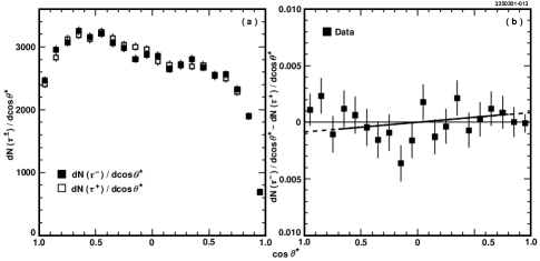
Figure 7: The pseudo-helicity distribution for charged taus is shown in a) while their difference is shown in b).

6 Search for Scalar Mediated $\tau$-Decays

We also search in a model independent way and without using the optimal observable $\xi$ for the presence of scalar mediated tau decays with the same final state as before. In the SM, the helicity angle $\theta_{\pi\pi^{0}}$, defined as the angle between the direction of the charges pion in the $\pi\pi^{0}$ rest frame and the direction of the $\pi\pi^{0}$ system in the $\tau$ rest frame, has a distribution appropriate to the exchange of a vector particle:

$${dN\over{d\,\cos\theta_{\pi\pi^{0}}}}\propto a+b\cos^{2}\theta_{\pi\pi^{0}}.$$ (4)

Including a non-SM scalar exchange leads to a $\cos\theta_{\pi\pi^{0}}$ term in the distribution, corresponding to S-P wave interference that is proportional to the non-SM complex coupling $\Lambda$:

$${dN\over{d\,\cos\theta_{\pi\pi^{0}}}}\propto a+(c_{1}Re(\Lambda)+c_{2}Im(\Lambda))\cos\theta_{\pi\pi^{0}}+b\cos^{2}\theta_{\pi\pi^{0}}.$$ (5)

Observation of a term proportional to $\cos\theta_{\pi\pi^{0}}$ would imply CP violation. However, the precise direction of the taus is unknown, due to the presence of a final state neutrinos, so the distribution in Eq. 5 cannot be formed. Instead, we use the ‘pseudo-helicity’ angle $\theta^{\ast}$, defined as the angle between the charged pion in the $\pi\pi^{0}$ rest frame and the direction of the $\pi\pi^{0}$ system in the lab frame. This doesn’t change the form of Eq. 5, just the coefficients.

The term in Eq. 5 containing $Im(\Lambda)$ changes sign for taus of opposite signs. Using the angle $\theta^{\ast}$, the difference between pseudo-helicity distributions for oppositely charged taus is given by

$${dN(\tau^{-})\over{d\,\cos\theta^{\ast}}}-{dN(\tau^{+})\over{d\,\cos\theta^{\ast}}}\sim 2c_{2}Im(\Lambda)\cos\theta^{\ast}.$$ (6)

The presence of a $\cos\theta^{\ast}$ term in such a distribution implies CP violation.

The data sample used for this search is the same as before. The pseudo-helicity distribution for charged taus is shown in figure 7a. The structure in the distributions is due to the variation in detection efficiency as a function of $\pi^{\pm}$ momentum and $\pi^{0}$ energy. To measure or constrain $Im(\Lambda)$ we need to determine the proportionality constant $c_{2}$. This is done with a procedure similar to the one used for the 3HDM case.

The difference in pseudo-helicity distributions is shown in figure 7b. The slope extracted from the data distribution is $c_{2}Im(\Lambda)=(4.2\pm 3.6)\times 10^{-4}$, consistent with zero. This leads to a constraint on $Im(\Lambda)$:

$$-0.033<Im(\Lambda)<0.089\ @\ 90\%\ {\rm CL}$$ (7)

Note that this result is consistent with, but less restrictive than our conservative limit shown in the first line of table 1. This is due to the use of a non-optimal CP-sensitive variable.

References

References

- [1] M.B. Einhorn and J. Wudka, hep-ph/0007285.
- [2] Y. Grossman, Nucl. Phys. B 426, 355 (1994).
- [3] C.H. Albright et al., Phys. Rev. D 21, 711 (1980).
- [4] S. Weinberg Phys. Rev. Lett. 37, 657 (1976).
- [5] D. Atwood and A. Soni Phys. Rev. D 45, 2405 (1992).
- [6] J. Gunion et al., Phys. Rev. Lett. 77, 5172 (1996).
- [7] CLEO Collaboration, to be published soon.
- [8] CLEO Collaboration, R. Balest em et al., Phys. Rev. D 47, 3671 (1993).