Inferring $\bar{\rho}$ and $\bar{\eta}$ of the CKM matrix
– A simplified, intuitive approach –

Abstract

This analysis is based on the same ideas and numerical inputs of the recent paper by Ciuchini et al. on the subject. Some approximations are applied, which make analytical calculations applicable in most of the work, thus avoiding Monte Carlo integration. The final result is practically identical to the one obtained by the more detailed numerical analysis.

1 Introduction

The “2000 CKM-triangle analysis” by Ciuchini et al. [1] is in my opinion the most accurate way to use consistently all pieces of experimental and theoretical information relevant to infer, within the framework of the Standard Model (SM), the parameters of the unitarity triangle. The basic idea is that beliefs (i.e. probabilities) on the value of each input quantity are propagated into beliefs about the output quantities, namely $\bar{\rho}$ and $\bar{\eta}$, and SM related quantities. The propagation is performed using the rules of logic applied to uncertain events, i.e. probability theory, without arbitrariness or “prescriptions”. All hypotheses are clearly stated and the influence on the results of reasonable variations of models and model parameters have been checked and found irrelevant (see Ref. [1] for details). Such a propagation of uncertainty, done by responsible people on physics quantities they feel knowledgeable about should not be confused with the kind of mathematical games described in Appendix A of Ref. [2]. In other words, when we say that the value of a quantity has 50% probability to lie in a certain region, given well defined hypotheses and with reasonably large flexibility of them, means that we are equally confident that it could be there or elsewhere. This is in contrast to “95% C.L. results” which should not be interpreted as 95% confidence on a certain statement (see e.g. Section 5.2 of Ref. [3], and the Conclusion of Ref.  [4] for an independent account).

The motivation of this note is to illustrate a simplified way to perform the analysis of Ref. [1]. In fact, the Monte Carlo integration used there could seem a bit mysterious. As well known, approximations usually loose accuracy, but often help in gaining awareness. And this is exactly the spirit of this note. Therefore, I have little to add here to phenomenology, experimental data and inferential framework of the analysis, and I point to Ref.  [1] and references therein.

The note is organized in the following way. In Section 2 the relations between CKM parameters are schematically recalled. In the following sections the reweighting effect on the points of the $\bar{\rho}$–$\bar{\eta}$ plane due to all pieces of information, is shown in detail. The final result is then compared to that of Ref. [1].

2 Uncertain constraints

The relations (1)–(4) of Ref. [1] can be written in the following way

$$\left|\frac{V_{ub}}{V_{cb}}\right|\hskip 26.17648pt\Rightarrow\hskip 85.35826pt\bar{\rho}^{2}+\bar{\eta}^{2} = a\hskip 105.2751pt(C_{1})$$

$$\Delta m_{d}\hskip 26.17648pt\Rightarrow\hskip 56.9055pt(1-\bar{\rho}^{2})+\bar{\eta}^{2} = b\hskip 105.2751pt(C_{2})$$

$$\left|\varepsilon_{K}\right|\hskip 31.2982pt\Rightarrow\hskip 45.52458pt\bar{\eta}\left[1+c\,(1-\bar{\rho})\right] = d\hskip 105.2751pt(C_{3})$$

$$(\mbox{mainly})\ \Delta m_{s}\hskip 28.45274pt\Rightarrow\hskip 56.9055pt(1-\bar{\rho}^{2})+\bar{\eta}^{2} = \frac{e}{\Delta m_{s}}\hskip 85.35826pt(C_{4})$$

where $a$,$b$, …$e$ are the constraint parameters, functions of many quantities; the most crucial of those determined experimentally are indicated on the left hand side of the equations. Note that the order of $C_{3}$ and $C_{4}$ is exchanged with respect to Eqs. (3)–(4) of Ref. [1]. This is because, since the present information concerning $\Delta m_{s}$ is of different quality with respect to the other quantities, the constraint $C_{4}$ needs a more careful treatment than the others, and it will be introduced after $C_{1}$–$C_{3}$. This is also the reason why $\Delta m_{s}$ appears explicitly in the constraint $C_{4}$.

In the ideal case all parameters are perfectly known, and the constraints would give curves in the $\bar{\rho}$–$\bar{\eta}$ plane. For example, $C_{1}$ would give a circle of radius $\sqrt{a}$. In other terms, due to this constraint all points of the circumference would be appear to us likely, unless there is any other experimental piece of information (or theoretical prejudice) to assign a different weight to different points. In the ideal case the p.d.f. describing our beliefs in the $\bar{\rho}$ and $\bar{\eta}$ values would be

$$f(\bar{\rho},\bar{\eta}\,|\,a)=\delta(\bar{\rho}^{2}+\bar{\eta}^{2}-a)\,,$$ (1)

with the Dirac delta meaning the limit of a very narrow p.d.f. concentrated on the circumference. Similar arguments hold for the parameters of the other constraints. Let us call them generically $p$ (the fact that $C_{3}$ depends on two parameters is conceptually irrelevant).

In the real case $p$ itself is not perfectly known. There are values which are more likely, and values which are less likely, classified by the p.d.f. $f(p)$. This means that, e.g. for the parameter $a$, we deal with an infinite number of circles, each having its weight $f(a)$. It follows that the points of the ($\bar{\rho}$, $\bar{\eta}$) plane get different weights.

The probability theory teaches us how to evaluate $f(\bar{\rho},\bar{\eta})$ taking into account all possible values of $p$:

$$f(\bar{\rho},\bar{\eta})=\int f(\bar{\rho},\bar{\eta}\,|\,p)\,f(p)\,\mbox{d}p\,.$$ (2)

Now the problem becomes how to evaluate $f(p)$, knowing that each $p$ depends on many input quantities $x_{i}$, denoted all together with $\mathbf{x}$ and described, in the most general case, by a joint p.d.f. $f(\mathbf{x})$. In most cases of practical interest, including the one we are discussing, each $x_{i}$ can be considered independent from the others, and the joint distribution simplifies to $f(\mathbf{x})\approx\prod f(x_{i})$. Calling $p(\mathbf{x})$ the function which relates $\mathbf{x}$ to $p$, $f(p)$ can be generally obtained as

$$f(p)=\int f(\mathbf{x})\,\delta(p-p(\mathbf{x}))\,\mbox{d}\mathbf{x}\,.$$ (3)

This integral, as well as the previous integrals, is usually performed by Monte Carlo techniques. The calculations can be simplified in the following way.

• First, we rely on the central limit theorem, assuming $f(p)$ to be Gaussian for all parameters (but with no constraint on the shape of $f(\bar{\rho},\bar{\eta})$ !).

• Expected value, standard (deviation) uncertainty and correlation are basically obtained by the usual propagation (see Ref. [5] for a similar application).

• Non linear effects in the propagation have been taken into account up to second order, using formulae of Ref. [6] (see this paper for the practical modeling of uncertainties and treatment of asymmetric cases).

• The correlation between $c$ and $d$ has been taken into account building a bi-variate $f(c,b)$.

As input quantities, Table 1 of Ref. [1] is used, combining properly (i.e. quadratically) the standard deviations. For example, for $\sigma\left(f_{B_{d}}\sqrt{\hat{B}_{B_{d}}}\right)$ expressed in MeV we obtain $\sqrt{25^{2}+(20/\sqrt{3})^{2}}=27.5$, where $20/\sqrt{3}$ stands for the standard deviation of a uniform distribution of half width 20 MeV. Note that, contrary to what some authors critical about Ref. [1] (and the related papers and presentations to conferences) think, I have the impression that my colleagues tend to make slightly conservative assessments of uncertainties. This feeling that I had a priori discussing with them is somewhat confirmed a posteriori by the excellent overlap of the partial inference by each constraint (as it will be shown in Fig. 9) and self-consistency between input parameters and values coming out of the inference obtained without the their contribution (see Ref. [1]).

The following results are obtained in terms of expected values and standard deviations (“$p=\mbox{E}(p)\pm\sigma(p)$”):

$$a = 0.145\pm 0.031$$ (4)

$$b = 0.73\pm 0.19$$ (5)

$$c = 3.4\pm 0.9$$ (6)

$$d = 1.23\pm 0.33\hskip 28.45274pt[\,\rho(c,d)=0.76\,]$$ (7)

$$e = 12.7\pm 1.2\,\mbox{ps}^{-1}$$ (8)

Only the correlation between $c$ and $b$ is relevant, and all others can be neglected, being below the 10% level (even that between $b$ and $e$, related by $\Delta m_{d}$, is negligible, being only +7%). The radii of the circles given by $C_{1}$ and $C_{2}$ are $0.38\pm 0.04$ and $0.85\pm 0.11$, respectively. These radii have the meaning of the sides of the unitarity triangle opposite to $\beta$ and $\gamma$, respectively, provided by $C_{1}$ and $C_{2}$ alone.

3 Partial results from $C_{1}$, $C_{2}$ and $C_{3}$

3.1 $\left|\frac{V_{ub}}{V_{cb}}\right|$

Applying our reasoning to the constraint given by $\left|\frac{V_{ub}}{V_{cb}}\right|$, we obtain

$$f(\bar{\rho},\bar{\eta}\,|\,C_{1}) = \int_{-\infty}^{+\infty}\!\delta(\bar{\rho}^{2}+\bar{\eta}^{2}-a)\,\frac{1}{\sqrt{2\,\pi}\,0.031}\,\exp{\left[-\frac{(a-0.145)^{2}}{2\,(0.031)^{2}}\right]}\,\mbox{d}a$$ (9)

$$= \frac{1}{\sqrt{2\,\pi}\,0.031}\,\exp{\left[-\frac{(\bar{\rho}^{2}+\bar{\eta}^{2}-0.145)^{2}}{2\,(0.031)^{2}}\right]}\,.$$ (10)

The contour plot shown in Fig. 1 for $\bar{\eta}\geq 0$. 3-D plots are given in Fig. 2 (in all figures “rho” and “eta” stand for $\bar{\rho}$ and $\bar{\eta}$).

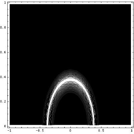
Figure 1: Contour plot of the p.d.f. of Fig. 2 for $\bar{\eta}\geq 0$. Note that contours are simply iso-p.d.f. levels obtained by 12 contour lines. In order to assign them a probabilistic meaning, one needs to evaluate the p.d.f. integrals inside the contours.

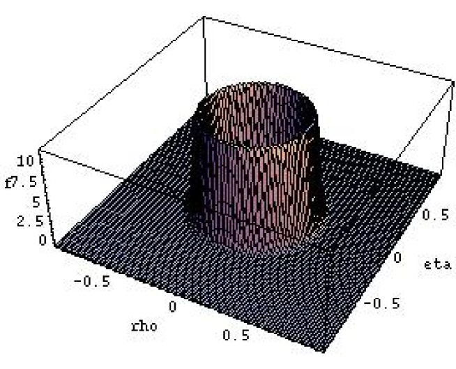
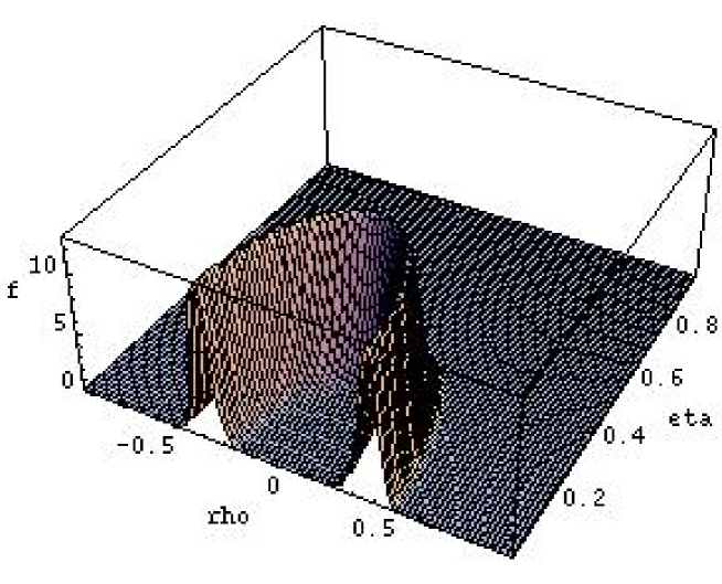
Figure 2: Probability density function of $\bar{\rho}$ and $\bar{\eta}$ obtained by the constraint given by $\left|\frac{V_{ub}}{V_{cb}}\right|$.

Note that the plot of Fig. 1 is obtained slicing $f(\bar{\rho},\bar{\eta}\,|\,C_{1})$ into 12 iso-p.d.f. contours, and hence the regions shown there have no straightforward probabilistic interpretation, since one should make the integrals of the p.d.f. inside the region. We leave it as an exercise for the interested readers.

3.2 $\Delta m_{d}$

From the $\Delta m_{d}$ we get

$$f(\bar{\rho},\bar{\eta}\,|\,C_{2}) = \int_{-\infty}^{+\infty}\!\delta((1-\bar{\rho})^{2}+\bar{\eta}^{2}-b)\,\frac{1}{\sqrt{2\,\pi}\,0.19}\,\exp{\left[-\frac{(b-0.73)^{2}}{2\,(0.19)^{2}}\right]}\,\mbox{d}b$$ (11)

$$= \frac{1}{\sqrt{2\,\pi}\,0.19}\,\exp{\left[-\frac{((1-\bar{\rho})^{2}+\bar{\eta}^{2}-0.73)^{2}}{2\,(0.19)^{2}}\right]}\,,$$ (12)

shown by 3-D plots in Fig. 4.

We can already combine the information from the two constraints, just remembering a condition stated in the second paragraph of section 2: In the ideal case we would consider the points of the circle equally likely if there were no other experimental or theoretical a priori information which would lead to assign different weights to the different points. But this is exactly what each partial inference does. Therefore, in order to combine the two constraints we just need to multiply the weights of each point and normalize the distribution:

$$f(\bar{\rho},\bar{\eta}\,|\,C_{1},C_{2})\propto f(\bar{\rho},\bar{\eta}\,|\,C_{1})\,f(\bar{\rho},\bar{\eta}\,|\,C_{2}).$$ (13)

The 3-D plot of the normalized distribution is shown in Fig. 3. We see that with these two constraints only there is still sign ambiguity, and, in particular, the distribution is specular with respect to the $\bar{\eta}=0$ axis.

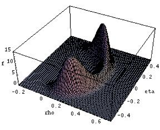
Figure 3: $f(\bar{\rho},\bar{\eta})$ from the constraints given by $\left|\frac{V_{ub}}{V_{cb}}\right|$ and $\Delta m_{d}$ .

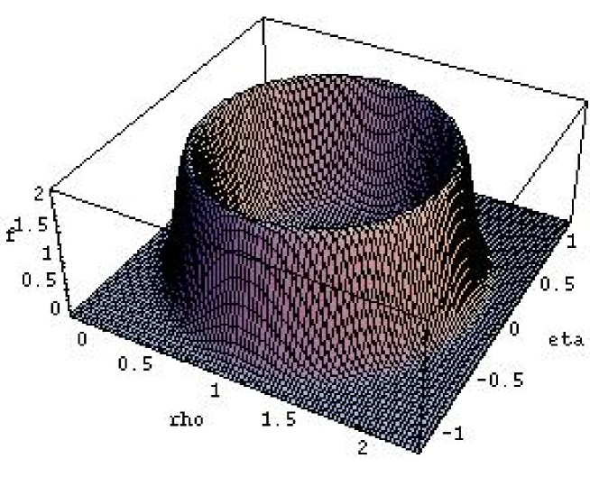
Figure 4: Probability density function of $\bar{\rho}$ and $\bar{\eta}$ obtained by the constraint given by $\Delta m_{d}$ .

3.3 $\left|\varepsilon_{K}\right|$

Since the third constraint depends on two strongly correlated parameters, we need to consider a joint bivariate Gaussian distribution:

$$f(c,d) = \frac{1}{2\,\pi\,\sigma_{c}\,\sigma_{d}\,\sqrt{1-\rho_{cd}^{2}}}\cdot\exp\left\{-\frac{1}{2\,(1-\rho_{cd}^{2})}\left[\frac{(x-\mu_{c})^{2}}{\sigma_{c}^{2}}\right.\right.$$ (14)

$$\left.\left.-2\,\rho_{cd}\,\frac{(c-\mu_{c})(d-\mu_{d})}{\sigma_{c}\,\sigma_{d}}+\frac{(d-\mu_{d})^{2}}{\sigma_{d}^{2}}\right]\right\}\,,$$

with $\mu_{c}=\mbox{E}[c]=3.4$, $\sigma_{c}=0.9$, $\mu_{d}=\mbox{E}[d]=1.23$, $\sigma_{d}=0.33$, and $\rho_{cd}=\rho(c,d)=0.76$. The integral

$$f(\bar{\rho},\bar{\eta}\,|\,C_{3})=\int\!\!\!\!\int_{-\infty}^{+\infty}\!\delta\left(\bar{\eta}\,[1+c\,(1-\bar{\rho})]-d\right)\,f(c,d)\,\mbox{d}c\,\mbox{d}c$$ (15)

can be still evaluated analytically but we omit here the final formula, just giving the 3-D plot of the resulting p.d.f. normalized in the region of interest (Fig. 5).

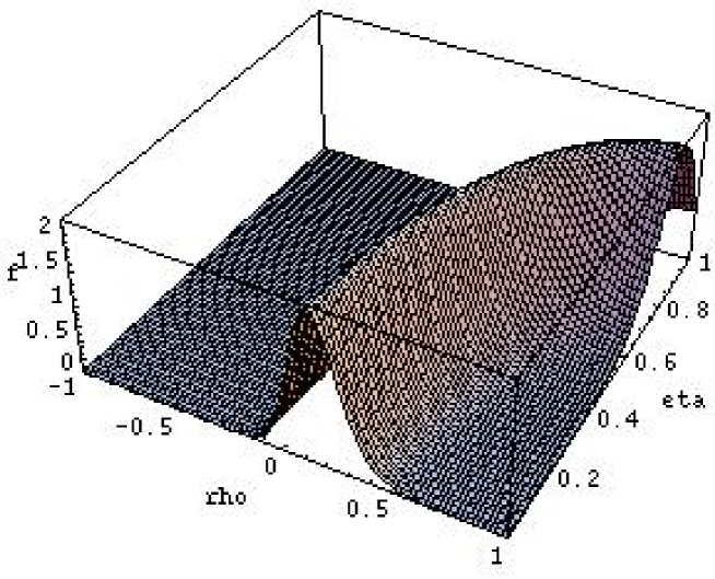
Figure 5: Probability density function of $\bar{\rho}$ and $\bar{\eta}$ obtained by the constraint given by $\left|\varepsilon_{K}\right|$.

4 Partial combinations of results ($C_{1}$, $C_{1}$ and $C_{3}$)

With this third reweighting, the resulting p.d.f. looses finally sign ambiguities, and becomes rather narrow, with respect to the initial space of possibilities. The 3-D plot is shown in Fig. 6.

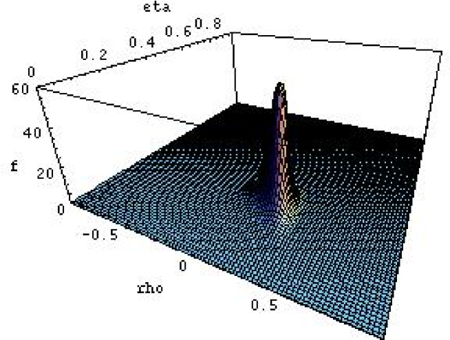
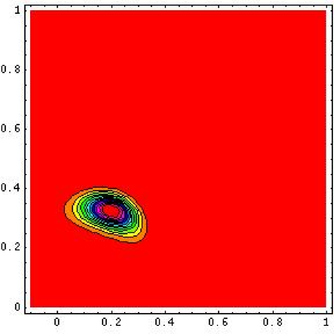
Figure 6: Probability density function and contour plot $f(\bar{\rho},\bar{\eta}\,|\,C1,C2,C3)$ obtained by the constraint given by $\left|\frac{V_{ub}}{V_{cb}}\right|$, $\bar{\eta}$ and $\Delta m_{d}$ (see remarks in text and in caption of Fig. 1 about the interpretation of the contour plot).

At this point we can evaluate expected value and standard uncertainty of the quantities of interest:

$$f(\bar{\rho},\bar{\eta}\,|\,C1,C2,C3)\hskip 14.22636pt\Rightarrow\hskip 28.45274pt\begin{array}[]{l}\left\{\begin{array}[]{l}\mbox{E}[\bar{\rho}]=0.19\\ \sigma(\bar{\rho})=0.07\end{array}\right.\\ \mbox{}\\ \left\{\begin{array}[]{l}\mbox{E}[\bar{\eta}]=0.32\\ \sigma(\bar{\eta})=0.04\end{array}\right.\end{array}$$ (16)

5 Including the experimental information about $\Delta m_{s}$

The treatment of the experimental information about $\Delta m_{s}$ cannot be done by the usual uncertainty propagation, just because the simplifying hypotheses (linearization and Gaussian model for $e/\Delta m_{s}$) do not hold. In fact, the likelihood, which has the role of reweighting the probability, is open, in the sense described in Section 7 of Ref. [7], i.e. it does not go to zero at both ends of the kinematical region ($\Delta m_{s}=0$ and $\Delta m_{s}=\infty$ in this case), as shown in the top plot of Fig. 7. The reason is simple: in this kind of measurement $\Delta m_{s}$ is not yet incompatible with $\infty$ (no oscillation). Though the open likelihood does not allow to renormalize the p.d.f. (unless strong priors forbidding high values are used), the likelihood can still be used to reweigh the points in the $\bar{\rho}$–$\bar{\eta}$ plane (see Refs. [5] and [8] for other examples and discussions about the $R$ function).

It is instructive to see how the reweighting of $\Delta m_{s}$ is turned into the reweighting of the square radius of circle centered in $\bar{\rho}=1$ and $\bar{\eta}=0$ given by the constraint $C_{4}$, i.e. $r^{2}=e/\Delta m_{s}$. This is illustrated in the central plot of Fig. 7. We see that the reflection of $R\rightarrow 0$ for $\Delta m_{s}<14$ ps^-1 essentially kills values above $r=1$, resulting in a strong sensitivity bound (in the sense of Ref. [7]) on the angle $\gamma$ of the CKM matrix, forced to be below 90^∘. The bottom plot of Fig. 7 shows the reweighting function in the $\bar{\rho}$–$\bar{\eta}$ plane.

For small values of $r^{2}$ the reweighting function is divergent, since the whole region of high $\Delta m_{s}$ is squeezed into a small region of $r^{2}$. This is no serious problem, since these points are already ruled out by the other constraints. The cutoff shown in the central and bottom plot of Fig. 7 is due to a cutoff at $\Delta m_{s}=100$ ps^-1. Note, moreover, that the values of $\Delta m_{s}$ preferred by the data (around 15–20 ps^-1) overlap well with the $\bar{\rho}$–$\bar{\eta}$ region indicated by the other constraints. Note also that even if one goes through the academic exercise of removing by hand the peak around 15–20 ps^-1, chopping $R$ to 1, the effect on the values of $r$ above 1 (and hence of $\gamma$ above 90^∘) does not change.

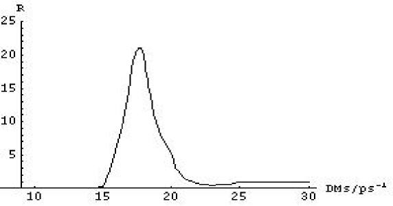
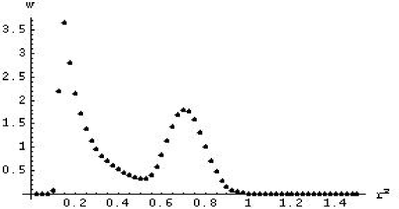
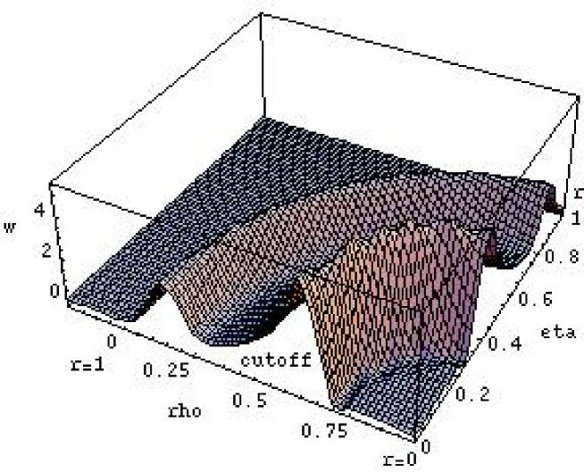
Figure 7: Top plot: likelihood of $\Delta m_{s}$ rescaled to the region of insensitivity. Central plot: reweighting factor of $r^{2}=e/\Delta m_{s}$. The peak just below 0.2 is an artifact of the cutoff in $\Delta m_{s}$ (see text). Bottom plot: same reweighting factor in the $\bar{\rho}$–$\bar{\eta}$ plane (note also here the low $r$ cutoff).

                               cutoff

6 Global combination and results

Reweighting $f(\bar{\rho},\bar{\eta}\,|\,C1,C2,C3)$ with $R$ function of $\Delta m_{s}$ we get the final result shown in Fig. 8.

Expected values and standard deviations are obtained by numerical integration. The result is

$$f(\bar{\rho},\bar{\eta}\,|\,C1,C2,C3,C4)\hskip 14.22636pt\Rightarrow\hskip 28.45274pt\begin{array}[]{l}\left\{\begin{array}[]{l}\mbox{E}[\bar{\rho}]=0.213\\ \sigma(\bar{\rho})=0.042\end{array}\right.\\ \mbox{}\hskip 99.58464pt\rho(\bar{\rho},\bar{\eta})=-0.12\\ \left\{\begin{array}[]{l}\mbox{E}[\bar{\eta}]=0.314\\ \sigma(\bar{\eta})=0.039\end{array}\right.\end{array}$$ (17)

practically identical to $\bar{\rho}=0.224\pm 0.038$ and $\bar{\eta}=0.317\pm 0.040$ given in Ref. [1] using the full Monte Carlo integration (obviously, those who pay attention the tenths of standard deviations should use the more accurate result of Ref. [1]).

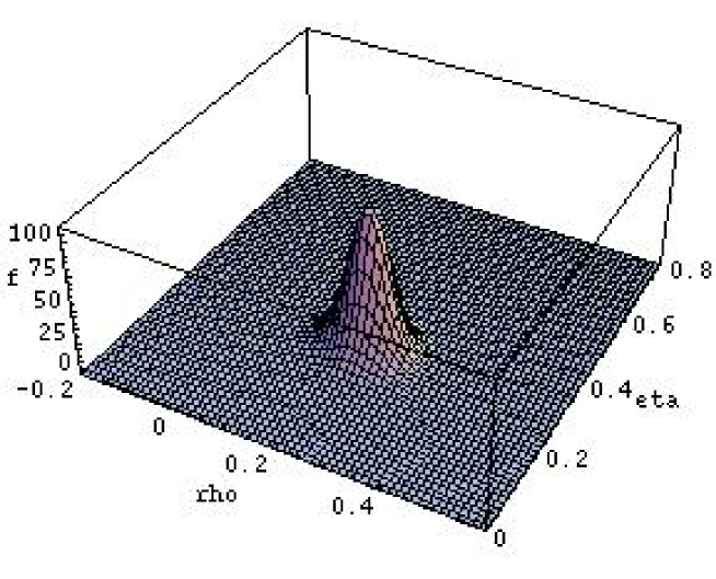
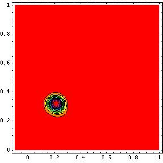
Figure 8: Probability density function and contour plot $f(\bar{\rho},\bar{\eta}\,|\,C1,C2,C3,C4)$ obtained by the constraint given by $\left|\frac{V_{ub}}{V_{cb}}\right|$, $\bar{\eta}$, $\Delta m_{d}$ and $\Delta m_{s}$ (see remarks in the text and in caption of Fig. 1 about the interpretation of the contour plot).

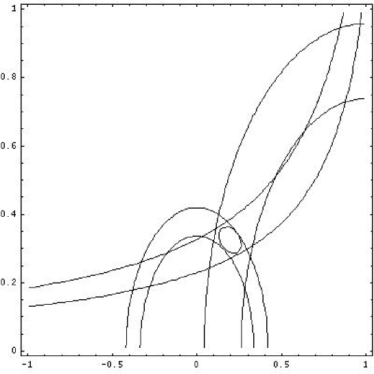
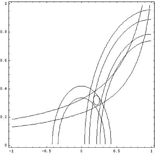
Figure 9: Top plot: $\Delta(\ln L)=1/2$ contours from the constraints $C_{1}$, $C_{2}$, $C_{3}$ and their combination. The bottom plot shows the effect of the experimental information on $\Delta m_{s}$, limited to the region of interest. The probability that $\bar{\rho}$ and $\bar{\eta}$ are both in the “ellipses” is about 37%.

$\bar{\eta}$










                                    $\left|\varepsilon_{K}\right|$



                                               $\left|\frac{V_{ub}}{V_{cb}}\right|$                    $\Delta m_{d}$



                      $\bar{\eta}$




                                                                                      $\Delta m_{s}$












                                                                                                      $\bar{\rho}$

It is interesting to show partial and global results as contour lines at $e^{-1/2}=0.61$ of the maximum of the reweighting functions, equivalent to the $\Delta(-\ln{L})=1/2$ or $\Delta\chi^{2}=1/2$ rules (I refer to Ref. [1] for the relation between “standard” methods based on $\chi^{2}$ minimization and the more detailed inferential scheme illustrated there). The top plot of Fig. 9 shows the contour “roads” given by the first three constraints, together with the (almost) ellipse of their combination. The probability that the values of $\bar{\rho}$ and $\bar{\eta}$ are both in the ellipse is about 37%. Instead, the projections of the ellipse on each axis gives an interval of about $68\%$ probability in each variable.

The bottom plot of Fig. 9 shows the effect of the constraint $C_{4}$. First we notice the perfect agreement between the $\Delta m_{d}$ and $\Delta m_{s}$ roads, indicating that the values of $\Delta m_{s}$ suggested by the data are absolutely consistent with the other constraints within the Standard Model. Furthermore, the effect of the $\Delta m_{s}$ on the “ellipse” of the final inference is to reshape the left side, increasing the value of $\bar{\rho}$ and decreasing its uncertainty, with almost no effect on $\bar{\eta}$, as also shown by the results (16) and (17).

7 Conclusion

The result of Ref. [1] has been reproduced, using some simplifying assumptions that allow most calculations to be performed analytically. The consistency of the pieces information on $\bar{\rho}$ and $\bar{\eta}$ coming from the different constraints, as well as that relating the constraints to the uncertain parameters of the theory (see Ref. [1] for details), is almost “too good”, suggesting that the final uncertainties are most likely somewhat overestimated.

We all are looking forward to the results of the $B$ factories and the next generation of experiments on the CKM matrix parameters, hoping to find evidence of new phenomenology that would give new vitality to particle physics.

It is a pleasure to thank my friends Achille et al. (Ref. [1]) which have dragged me into this business.

References

- [1] M. Ciuchini et al., hep-ex/0012308, and references therein for an introduction to phenomenology and analysis approach, input values and detailed discussion of results.
- [2] A. Hocker et al., hep-ph/0104062.
- [3] G. D’Agostini, physics/9811046.
- [4] A.L. Read, CERN-OPEN-2000-205 (also in CERN Report 2000-005, pp. 81–99).
- [5] G. D’Agostini and G. Degrassi, Eur. Phys. J. C10 (1999) 633.
- [6] G. D’Agostini and M. Raso, hep-ex/0002056.
- [7] G. D’Agostini, hep-ex/0002055 (also in CERN Report 2000-005, pp. 3–23).
- [8] G. D’Agostini and P. Astone, hep-ex/9909047.