BNL-NT-01/14

RBRC-193

July 2001

Towards a global analysis

of polarized parton distributions

Marco Stratmann^a,b and Werner Vogelsang^c,d

^aInstitut für Theoretische Physik, Universität Regensburg,
D-93040 Regensburg, Germany

^bC.N. Yang Institute for Theoretical Physics, SUNY at Stony Brook,
Stony Brook, New York 11794 – 3840, U.S.A.

^cPhysics Department, Brookhaven National Laboratory,
Upton, New York 11973, U.S.A.

^dRIKEN-BNL Research Center, Bldg. 510a, Brookhaven National Laboratory,
Upton, New York 11973 – 5000, U.S.A.

We present a technique for implementing in a fast way, and without any approximations, higher-order calculations of partonic cross sections into global analyses of parton distribution functions. The approach, which is set up in Mellin-moment space, is particularly suited for analyses of future data from polarized proton-proton collisions, but not limited to this case. The usefulness and practicability of this method is demonstrated for the semi-inclusive production of hadrons in deep-inelastic scattering and the transverse momentum distribution of “prompt” photons in $pp$ collisions, and a case study for a future global analysis of polarized parton densities is presented.

1 Introduction

High-energy spin physics has been going through a period of great popularity and rapid developments ever since the measurement of the proton’s spin-dependent deep-inelastic structure function $g_{1}^{p}$ by the EMC [1] more than a decade ago. As a result of combined experimental and theoretical efforts, we have gained some fairly precise information concerning, for example, the total quark spin contribution to the nucleon spin. Yet, many other interesting and important questions, most of which came up in the wake of the EMC measurement, remain unanswered so far, the most prominent “unknown” being the nucleon’s spin-dependent gluon density, $\Delta g$. Also, polarized inclusive deep-inelastic scattering (DIS) data do not provide enough information for a complete separation of the distributions for the different quark and anti-quark flavors $u,\bar{u},d,\bar{d},s$, and $\bar{s}$. Here in particular a possible flavor asymmetry in the nucleon’s light sea, $\Delta\bar{u}-\Delta\bar{d}\neq 0$, has attracted quite some interest, and several models have been proposed recently [2, 3, 4]. Current and future dedicated spin experiments are expected to vastly broaden our understanding of the nucleon spin structure by studying reactions that give further access to its spin-dependent parton distributions, among them $\Delta g$ and $\Delta\bar{u}$, $\Delta\bar{d}$. In addition to lepton-nucleon scattering, there will also be for the first time information coming from very inelastic polarized $pp$ collisions at the BNL Relativistic Heavy-Ion Collider RHIC [5].

Having available at some point in the near future spin data on various different reactions, one needs to tackle the question of how to determine the polarized parton densities from the data. Of course, this problem is not at all new: in the unpolarized case, several groups perform such “global analyses” of the plethora of data available there [6, 7]. The strategy is in principle clear: an ansatz for the parton distributions at some initial scale $\mu_{0}$, given in terms of appropriate functional forms with a set of free parameters, is evolved to a scale $\mu_{F}$ relevant for a certain data point for a certain cross section. Then the parton densities at scale $\mu_{F}$ are used to compute the theoretical prediction for the cross section, and a $\chi^{2}$ value is assigned that represents the quality of the comparison to the experimental point. This is done for all data points to be included in the analysis, and subsequently the parameters in the ansatz for the parton distribution functions are varied, until eventually a minimum in $\chi^{2}$ is reached.

In practice, this approach is not fully viable if the partonic scattering is treated beyond the lowest order of perturbation theory. The numerical evaluation of the hadronic cross section at higher orders is usually a rather time-consuming procedure as it often requires several tedious numerical integrations, not only for the convolutions with the parton densities, but also for the phase space integrations in the partonic cross section. The fitting procedure outlined above, on the other hand, usually requires thousands of computations of the cross section for any given data point, and so the computing time required for a fit easily becomes excessive even on modern workstations. We note that for practically all reactions of interest in the unpolarized and polarized cases the first-order QCD corrections to the respective partonic cross sections are known by now. They are generally indispensable in order to arrive at a firmer theoretical prediction for hadronic cross sections; for instance the dependence on the unphysical factorization and renormalization scales is reduced when going to higher orders in the perturbative expansion. Only then can one reliably extract information on the parton distribution functions.

In the unpolarized case, a way to get around this problem is based on the fact that the parton densities are already known here rather accurately [6, 7]. Their gross features are basically determined by the wealth of very precise DIS data which cover a wide kinematical range in the momentum fraction $x$ and the scale $\mu_{F}\simeq Q$. As a consequence, the theory answer for a certain cross section is expected to change in a very predictable way when going from the lowest-order Born level to the first-order approximation. It is then possible to pre-calculate a set of correction factors $K_{i}$ ($i$ running over the data points), and to simply multiply them in each step of the fitting procedure to the lowest-order approximation for the cross section, the latter being usually much faster to evaluate than that involving higher order terms. The $K_{i}$ usually hardly change at all from one set of parton distributions to another, and in any case one may update them if necessary at certain stages of the fitting procedure.

It should be noted, however, that this way of treating next-to-leading order (NLO) corrections in a fit is not necessarily adequate in all cases of interest. In particular if one is interested in extracting information about the gluon density at large values of $x$, where it is only rather poorly constrained at the moment, the correction factors $K_{i}$ cannot be reliably pre-calculated, and they may vary considerably during the fitting procedure. It is therefore desirable to incorporate NLO cross sections without any approximations in future analyses of parton densities.

In the polarized case it is in general not at all clear whether a strategy based on correction factors $K_{i}$ will work. Here, the parton densities are known with much less accuracy so far. It is therefore not possible to pre-calculate higher-order correction factors that one would be able to keep fixed throughout the fit, while using “fast” lowest-order expressions for the partonic cross sections. For instance, even though it is well known that for a sizable $\Delta g$ the $q+g\to\gamma+q$ Compton subprocess is the dominant contributor to the transverse momentum distribution of a “prompt” photon in the kinematical region of interest, this is by no means the case if $\Delta g$ happens to be small, in which case all other channels, even genuine NLO ones, may become equally important. In addition, the spin-dependent parton distributions, as well as the polarized partonic cross sections, may have zeros in the kinematical regions of interest, near which the predictions at lowest order and the next order will show marked differences. Therefore, even if the correction factors are updated at times during the fitting procedure, the convergence of the fit is not warranted. Conversely, if one updates the $K_{i}$ frequently, the fit will become too slow again.

Clearly, in the polarized case, the goal must be to find a way of implementing efficiently, and without approximations, the exact NLO expression for any hadronic cross section such as the prompt photon cross section into the fitting procedure. As will be shown in the next Section, this can be achieved in a very simple and straightforward way by going to Mellin-$n$ moment space. A technique of this sort was first used for the case of jet production in DIS as a means of extracting information about the unpolarized gluon density [8]. The relevant generalization to hadron-hadron scattering, which is more involved and requires a “double Mellin transform” was recently provided in [9]. However, [9] focuses on the formalism and the technical aspects of the Mellin transformation, rather than on its actual practicability, and the usefulness in a global QCD analysis has never been demonstrated.

Before we demonstrate in some detail the potential of the Mellin technique in praxis for two examples relevant for future global analyses of polarized parton densities, which is the main thrust of this paper, we start off in the next Section by rederiving the required formalism in an easy and transparent way. In Section 3 we will consider first the semi-inclusive production of hadrons in polarized DIS as the simplest application of the Mellin technique. The $n$ moments of the partonic cross sections can be taken analytically in this case. Due to the subsequent fragmentation of a final state parton into the observed hadron, semi-inclusive DIS (SIDIS) is sensitive to different flavor combinations than inclusive DIS data. It has also the advantage that we have already data at our disposal [10, 11] which can be analysed in terms of a possible flavor asymmetry $\Delta\bar{u}-\Delta\bar{d}$ of the light sea. As a second example we study the production of a prompt photon at high transverse momentum $p_{T}$ in $pp$ collisions at RHIC in Section 4. Its sensitivity to the gluon distribution via the LO Compton subprocess, which, along with the cleanliness of the prompt photon signal, is the reason why this process will be the flagship measurement of $\Delta g$ at RHIC [5]. As a first case study for future global analyses we also carry out a “toy” analysis of DIS and projected prompt photon data to highlight the power of future RHIC $pp$ data to pin down $\Delta g$. We briefly summarize the main results in Section 5.

2 Hadronic Cross Sections and the Mellin Moment Technique

The factorization theorem [12] ensures that in the presence of a hard scale in a reaction the corresponding (spin-dependent) hadronic cross section can be written as a sum over “convolutions” of parton densities with partonic hard-scattering cross sections. The latter are perturbatively calculable and are specific to the reaction under consideration. The parton distributions, which for spin-dependent interactions contain the desired information on the nucleon’s spin structure, depend on long-distance phenomena. However, they are universal: a single set of distributions for (anti-)quarks $u,\bar{u},d,\bar{d},s,\bar{s},\ldots$ and gluons $g$, predicts all data sets simultaneously.

To be specific, for a general spin-dependent cross section in longitudinally polarized $pp$ collisions, differential in a certain observable $O$ and integrated over experimental bins in other kinematical variables $T$, one has

$$\frac{d\Delta\sigma^{H}}{dO} \equiv \frac{1}{2}\left[\frac{d\sigma^{H}}{dO}(++)-\frac{d\sigma^{H}}{dO}(+-)\right]$$

$$= \sum_{a,b,c}\,\int_{\mathrm{e}xp-bin}dT\,\int_{x_{a}^{\mathrm{m}in}}^{1}dx_{a}\int_{x_{b}^{\mathrm{m}in}}^{1}dx_{b}\int_{z_{c}^{\mathrm{m}in}}^{1}dz_{c}\,\,\Delta f_{a}(x_{a},\mu_{F})\,\Delta f_{b}(x_{b},\mu_{F})D_{c}^{H}(z_{c},\mu_{F}^{\prime})\,$$

$$\times\,\frac{d\Delta\hat{\sigma}_{ab}^{c}}{dOdT}(x_{a}P_{A},x_{b}P_{B},P_{H}/z_{c},T,\mu_{R},\mu_{F},\mu_{F}^{\prime})\;,$$

where the arguments $(++)$ and $(+-)$ in the first line of Eq. (2) refer to the helicities of the incoming hadrons $A$ and $B$. The $\Delta f_{i}$ are the spin-dependent parton distributions, defined as

$$\Delta f_{i}(x,\mu_{F})\equiv f_{i}^{+}(x,\mu_{F})-f_{i}^{-}(x,\mu_{F})\;,$$ (2)

where $f_{i}^{+}$ ($f_{i}^{-}$) denotes the number density of a parton-type $f_{i}$ with helicity ‘+’ (‘$-$’) in a proton with positive helicity, carrying the fraction $x$ of the proton’s momentum. The $D_{c}^{H}(z,\mu_{F}^{\prime})$ represent the unpolarized fragmentation functions. They parameterize the probability that a parton $c$ fragments into the observed final state $H$, e.g., a charged pion, with momentum $P_{H}=z\,p_{c}$. For some observables, such as (di-)jets, there is no need for a fragmentation function in Eq. (2).

The scales $\mu_{F}$ and $\mu_{F}^{\prime}$ are the factorization scales for initial and final state collinear singularities, respectively, and reflect the certain amount of arbitrariness in the separation of short-distance and long-distance physics embodied in Eq. (2). Even though the parton densities (fragmentation functions) cannot presently be derived from first principles, their dependence on $\mu_{F}$ ($\mu_{F}^{\prime}$) is calculable perturbatively in terms of the “DGLAP” evolution equations [13], allowing to relate their values at one scale to their values at any other $\mu_{F}$ ($\mu_{F}^{\prime}$). The other scale, $\mu_{R}$, in Eq. (2) is the renormalization scale, introduced in the procedure of renormalizing the strong coupling constant. Finally, the sum in Eq. (2) is over all contributing partonic channels $a+b\to c+X$, with $d\Delta\hat{\sigma}_{ab}^{c}$ the associated partonic cross section, defined in complete analogy with the first line of Eq. (2), the helicities now referring to partonic ones:

$$d\Delta\hat{\sigma}_{ab}^{c}\equiv\frac{1}{2}\Bigg{[}d\hat{\sigma}_{ab}^{c}(++)-d\hat{\sigma}_{ab}^{c}(+-)\Bigg{]}\;.$$ (3)

As mentioned earlier, the $d\Delta\hat{\sigma}_{ab}^{c}$ are perturbative, that is, they have the expansion

$$d\Delta\hat{\sigma}_{ab}^{c}=d\Delta\hat{\sigma}_{ab}^{c,(0)}+\left(\frac{\alpha_{s}}{\pi}\right)d\Delta\hat{\sigma}_{ab}^{c,(1)}+\left(\frac{\alpha_{s}}{\pi}\right)^{2}d\Delta\hat{\sigma}_{ab}^{c,(2)}+\ldots\;\,.$$ (4)

It should be noted that lepton-hadron reactions are also included in Eq. (2) by simply setting $\Delta f_{b}(x_{b},\mu_{F})=\delta(1-x_{b})$. We will consider this example in some detail in Section 3 as it is the simplest application of the Mellin moment technique which we are going to advocate in the following as a straightforward tool to extract information about parton densities from a global QCD analysis.

For the polarized parton distribution functions, the Mellin moments are defined as

$$\Delta f_{i}^{n}(\mu)\equiv\int_{0}^{1}dx\;x^{n-1}\Delta f_{i}(x,\mu)\;.$$ (5)

It is well known [14] that the evolution equations for the the parton densities become particularly simple in Mellin-$n$ space, since the convolutions occuring in the $x$-space equations factorize into simple products under moments. This allows for a straightforward analytic solution of the differential evolution equations, see, e.g., [14]. In fact, several of the NLO evolution codes used for parton density analyses in the unpolarized and polarized cases are set up in Mellin-$n$ space. After evolving from one scale to another in moment space, the evolved parton distributions in Bjorken-$x$ space are recovered by an inverse Mellin transform, given by

$$\Delta f_{i}(x,\mu)=\frac{1}{2\pi i}\int_{{\cal C}_{n}}dn\;x^{-n}\Delta f_{i}^{n}(\mu)\;,$$ (6)

where ${\cal C}_{n}$ denotes a contour in the complex $n$ plane that has an imaginary part ranging from $-\infty$ to $\infty$ and that intersects the real axis to the right of the rightmost poles of the $\Delta f_{i}^{n}(\mu)$. The evolution of the time-like fragmentation functions can be treated in a very similar way in Mellin space as well.

The crucial, but simple, step in applying moment techniques to Eq. (2) is to express the $\Delta f_{i}(x_{i},\mu_{F})$ by their Mellin inverses in Eq. (6) [9]. One subsequently interchanges integrations and arrives at

$$\frac{d\Delta\sigma^{H}}{dO} = \frac{1}{(2\pi i)^{2}}\sum_{a,b,c}\,\int_{{\cal C}_{n}}dn\;\int_{{\cal C}_{m}}dm\;\Delta f_{a}^{n}(\mu_{F})\,\Delta f_{b}^{m}(\mu_{F})$$ (7)

$$\times\,\int_{\mathrm{exp-bin}}dT\,\int_{x_{a}^{\mathrm{m}in}}^{1}dx_{a}\int_{x_{b}^{\mathrm{m}in}}^{1}dx_{b}\int_{z_{c}^{\mathrm{m}in}}^{1}dz_{c}\,\,x_{a}^{-n}x_{b}^{-m}\;D_{c}^{H}(z_{c},\mu_{F}^{\prime})$$

$$\times\,\frac{d\Delta\hat{\sigma}_{ab}^{c}}{dOdT}(x_{a}P_{A},\,x_{b}P_{B}\,,P_{H}/z_{c},T,\,\mu_{R},\mu_{F},\mu_{F}^{\prime})$$

$$\equiv \sum_{a,b}\,\int_{{\cal C}_{n}}dn\;\int_{{\cal C}_{m}}dm\;\Delta f_{a}^{n}(\mu_{F})\,\Delta f_{b}^{m}(\mu_{F})\;\Delta\tilde{\sigma}_{ab}^{H}(n,m,O,\mu_{R},\mu_{F})\;.$$ (8)

One can now pre-calculate the quantities $\Delta\tilde{\sigma}_{ab}^{H}(n,m,O,\mu_{R},\mu_{F})$, which do not depend at all on the parton distribution functions, prior to the fit for a specific set of the two Mellin variables $n$ and $m$, for each contributing subprocess and in each experimental bin. Effectively, one has to compute the cross sections with complex “dummy” parton distribution functions $x_{a}^{-n}\,x_{b}^{-m}$. We emphasize that all the tedious and time-consuming integrations are already dealt with in the calculation of the $\Delta\tilde{\sigma}_{ab}^{H}(n,m,O,\mu_{R},\mu_{F})$. We have included the integration over the fragmentation function $D_{c}^{H}$ and the summation over the final state parton $c$ in the definition of the pre-calculated quantities $\Delta\tilde{\sigma}_{ab}^{H}$. This also implies that $\Delta\tilde{\sigma}_{ab}^{H}$ does not depend anymore on the choice for $\mu_{F}^{\prime}$ apart from some residual dependence which is of higher order in $\alpha_{s}$. Usually the fragmentation functions are taken from “elsewhere”, i.e., $e^{+}e^{-}$ data, rather than being fitted simultaneously with the parton densities. We note, however, that one can also replace $D_{c}^{H}$ by their Mellin inverse according to Eq. (6). In that case the pre-calculated quantities would depend on three Mellin variables.

The double inverse Mellin transformation which finally links the parton distributions with the pre-calculated $\Delta\tilde{\sigma}_{ab}^{H}(n,m,O,\mu_{R},\mu_{F})$ of course still needs to be performed in each step of the fitting procedure. However, the integrations over $n$ and $m$ in Eq. (8) are extremely fast to perform by choosing the values for $n,m$ in $\Delta\tilde{\sigma}_{ab}^{H}(n,m,O,\mu_{R},\mu_{F})$ on the contours ${\cal C}_{n}$, ${\cal C}_{m}$ simply as the supports for a Gaussian integration. The point here is that the integrand in $n$ and $m$ falls off very rapidly as $|n|$ and $|m|$ increase along the contour, for two reasons: first, each parton distribution function is expected to fall off at least as a power $(1-x)^{3}$ at large $x$, which in moment space converts into a fall-off of $\sim 1/n^{4}$ or higher. Secondly, we may choose contours in moment space that are bent by an angle $\alpha-\pi/2$ with respect to the vertical direction; a possible choice is shown in Fig. 1. Then, for large $|n|$ and $|m|$, $n$ and $m$ will acquire large negative real parts, so that $(x_{a})^{-n}$ and $(x_{b})^{-m}$ decrease exponentially along the respective contours. This helps for the numerical convergence of the calculation of the $\Delta\tilde{\sigma}_{ab}^{H}(n,m,O,\mu_{R},\mu_{F})$ and also gives them a rapid fall-off at large arguments. We note that no new poles in $n$ and $m$, beyond those already present in the moments of the parton distribution functions, are introduced by the $\Delta\tilde{\sigma}_{ab}^{H}(n,m,O,\mu_{R},\mu_{F})$ [9].

We note that if one wishes to integrate also over an experimental bin in $O$ in Eq. (7), a potential complication arises if the hard scale $\mu_{F}$ in the parton distribution functions depends explicitly on $O$. This makes it impossible to straightforwardly include the $O$ integration in the pre-calculation of the $\Delta\tilde{\sigma}_{ab}^{H}$. A typical example for $O$, which often appears in practice, is the transverse momentum $p_{T}$ of an observed jet, hadron, or prompt photon. In this case, the $O$ dependence of $\mu_{F}$ is, however, not a serious limitation [8]: the logarithmic dependence of the parton densities on $\mu_{F}$ is much weaker than the overall $p_{T}$ dependence of the cross section. Therefore, it is always possible to choose a bin-average of $p_{T}$ as the scale in the parton densities. Alternatively, one could choose not to include the $p_{T}$ integration in the $\Delta\tilde{\sigma}_{ab}^{H}$ and to construct grids of somewhat larger size, taken at a small number of support points for a simple Gaussian integration over the $p_{T}$ bin. A further possibility [9] is to absorb also the evolution of the parton densities from their initial scale $\mu_{0}$ to $\mu_{F}$ into the $\Delta\tilde{\sigma}_{ab}^{H}$, which in moment space simply enters in the form of exponentials involving the anomalous dimensions, see, e.g., [14]. This procedure, which is somewhat more involved, would eliminate any complication related to $\mu_{F}\sim{\cal O}(p_{T})$. Anyway, the experiments will usually quote results for the $p_{T}$-differential cross section at the $p_{T}$-average over the bin, which of course is exactly what we have considered in Eqs. (7), (8). In the latter case it is also easily possible to organize the grids in such a way that the renormalization and/or factorization scales can be varied during the fit, by simply taking the (logarithmic) dependence on $\mu_{R,F}$ and the strong coupling $\alpha_{s}(\mu_{R})$ out of the partonic cross sections beforehand.

Figure 1: Contours in complex Mellin-$n,m$ spaces for the calculation of the double Mellin inverse in Eq. (8). $r_{n}$ and $r_{m}$ denote the rightmost poles of the integrand in $n$ and $m$, respectively, and the $c_{i}$ the intersections with the real axis.

As a technical sidestep, we give an explicit expression for the double inverse transform in Eq. (8) for the contours depicted in Fig. 1. To this end, we parameterize the various segments in Fig. 1 by

$$n=c_{n}+u_{n}\,{\rm e}^{\pm i\alpha}\;\;\;{\mathrm{a}nd}\;\;\;m=c_{m}+u_{m}\,{\rm e}^{\pm i\alpha}\;,$$ (9)

where $u_{n,m}\in[0,\infty]$ and the sign of $\alpha$ has to be chosen appropriately for the branches of the contours. We then find

$$\frac{d\Delta\sigma^{H}}{dO} = -\frac{1}{2\pi^{2}}\sum_{a,b}\,{\rm Re}\Bigg{[}\int_{0}^{\infty}du_{n}\int_{0}^{\infty}du_{m}\;\Delta f_{a}^{n}(\mu_{F})\,$$

$$\times\Bigg{\{}{\rm e}^{2i\alpha}\Delta f_{b}^{m}(\mu_{F})\,\Delta\tilde{\sigma}_{ab}^{H}(n,m,O,\mu_{R},\mu_{F})-\left(\Delta f_{b}^{m}(\mu_{F})\right)^{*}\,\Delta\tilde{\sigma}_{ab}^{H}(n,m^{*},O,\mu_{R},\mu_{F})\Bigg{\}}\Bigg{]}\;,$$

where the asterisk denotes the complex conjugate, and where we have made use of $\Delta f_{b}^{m^{*}}(\mu_{F})=\left(\Delta f_{b}^{m}(\mu_{F})\right)^{*}$, since the $\Delta f_{i}(x,\mu)$ are real functions. This identity also implies that there is no need to separately compute the moments of the parton densities at the complex conjugate values $n^{*},m^{*}$, which has a further positive effect on the computing time required for performing the Mellin inverses. In addition, there is no need to provide separate grids for $\Delta\tilde{\sigma}_{ab}^{H}(n^{*},m,O,\mu_{R},\mu_{F})$ and $\Delta\tilde{\sigma}_{ab}^{H}(n^{*},m^{*},O,\mu_{R},\mu_{F})$.

Before proceeding, we reemphasize that the idea outlined above of reverting to Mellin moment space in the implementation of any higher-order cross section into parton density fits is not entirely new, but was first developed in Refs. [8, 9]. The example considered in [8] was jet production in DIS, which offers the simplification of being only linear in the parton distribution functions. There is a difference between our approach and that of Ref. [8] in practical terms: in the language of our example in Eq. (7), Ref. [8] would insert a factor $(x_{a}^{\rm min})^{n}\,(x_{b}^{\rm min})^{m}$ in the integrands for the $x_{a}$ and $x_{b}$ integrations, while undoing this operation through a factor $(x_{a}^{\rm min})^{-n}\,(x_{b}^{\rm min})^{-m}$ in the $n$ and $m$ integrands. Even though obviously equivalent mathematically, the disadvantage of this procedure is that the resulting factors $(x_{a}^{\rm min}/x_{a})^{n}$, $(x_{b}^{\rm min}/x_{b})^{m}$ in the $x_{a}$, $x_{b}$ integrands will now grow exponentially along the contours in Mellin space, making it numerically much more cumbersome [8] to perform the $x_{a}$ and $x_{b}$ integrations yielding the $\Delta\tilde{\sigma}_{ab}^{H}(n,m,O,\mu_{R},\mu_{F})$. As a matter of fact, the actual extension of the method of Ref. [8] to the case of hadronic collisions involving bilinear combinations of parton distributions appears difficult. The generalization of [8] to hadron-hadron scattering, without the shortcomings mentioned above, was first provided in [9]. The difference between our organization of the expression in Eq. (8) and Ref. [9] is the choice of the contour. Reference [9] fully exploits the freedom in deforming the contours for the inverse Mellin transform and constructs a “surface of steepest descent” which in principle has the best numerical convergence properties but is difficult to parameterize. Instead we stick to the simple contours in Fig. 1 which, as we will show below, turn out to be sufficient to obtain numerical agreement between Eqs. (2) and (8) of far better than 1% for all applications we are going to consider. We should also note that in [9] the usefulness of the Mellin transform method was not demonstrated in practice.

3 Semi-Inclusive Deep-Inelastic Scattering

As a first application for the Mellin transform technique outlined in the previous Section we consider the semi-inclusive production of a hadron $H$ in DIS. SIDIS starts at the Born level with the LO reaction $\gamma^{*}q\rightarrow q$. The NLO ${\cal O}(\alpha_{s})$ corrections also comprise the processes $\gamma^{*}q\rightarrow qg$ and $\gamma^{*}g\rightarrow q\bar{q}$ and have been calculated in the spin-dependent case in the $\overline{\mathrm{MS}}$ scheme in [15]. In each case one of the final state partons subsequently fragments into the observed hadron $H$. As in the fully inclusive case, the expression for the cross section is given by a single structure function $g_{1}^{H}(x,z,Q)$:

$$\frac{d\Delta\sigma^{H}}{dx\,dy\,dz}=\frac{4\pi\alpha^{2}}{Q^{2}}(2-y)\,g_{1}^{H}(x,z,Q)\;.$$ (11)

To NLO in $\alpha_{s}$, $g_{1}^{H}$ can be written as [15, 16]

$$2\,g_{1}^{H}(x,z,Q) = \sum_{q=u,\bar{u},\ldots,\bar{s}}\!\!\!e_{q}^{2}\;\Bigg{[}\Delta q\left(x,\mu_{F}\right)D_{q}^{H}\left(z,\mu_{F}^{\prime}\right)+\frac{\alpha_{s}(\mu_{R})}{2\pi}\int_{x}^{1}\frac{d\hat{x}}{\hat{x}}\int_{z}^{1}\frac{d\hat{z}}{\hat{z}}\Bigg{\{}$$ (12)

$$\Delta q\left(\frac{x}{\hat{x}},\mu_{F}\right)\Delta C_{qq}^{(1)}(\hat{x},\hat{z},\frac{\mu_{F}}{Q},\frac{\mu_{F}^{\prime}}{Q})D_{q}^{H}\left(\frac{z}{\hat{z}},\mu_{F}^{\prime}\right)+$$

$$\Delta q\left(\frac{x}{\hat{x}},\mu_{F}\right)\Delta C_{gq}^{(1)}(\hat{x},\hat{z},\frac{\mu_{F}}{Q},\frac{\mu_{F}^{\prime}}{Q})D_{g}^{H}\left(\frac{z}{\hat{z}},\mu_{F}^{\prime}\right)+$$

$$\Delta{g}\left(\frac{x}{\hat{x}},\mu_{F}\right)\Delta C_{qg}^{(1)}(\hat{x},\hat{z},\frac{\mu_{F}}{Q},\frac{\mu_{F}^{\prime}}{Q})D_{q}^{H}\left(\frac{z}{\hat{z}},\mu_{F}^{\prime}\right)\Bigg{\}}\Bigg{]}$$

with $x$ and $y$ denoting the usual DIS scaling variables ($Q^{2}=-q^{2}=xyS$), and where [17, 18] $z\equiv p_{H}\cdot p_{N}/p_{N}\cdot q$. Eq. (12) and the variable $z$ only apply to hadron production in the current fragmentation region characterized by positive values for the Feynman variable $x_{F}$. All NLO $\overline{\mathrm{MS}}$ partonic coefficient functions $\Delta C_{ij}^{(1)}$ are collected in App. C of [15]. They are non-trivial functions of $x$ and $z$ such that the $x$ and $z$ dependences of the cross section do not factorize into separate functions. Therefore the inclusion of the NLO corrections seems to be indispensable for a reliable extraction of parton densities from SIDIS.

Due to the double convolutions appearing in Eq. (12) and the fact that the coefficient functions contain mathematical distributions as $x\rightarrow 1$ and/or $z\rightarrow 1$, the direct use of Eq. (12) in a global analysis of parton densities is rather time consuming and awkward, though not impossible [19] since the partonic coefficient functions are still fairly simple. SIDIS has the advantage, however, that the Mellin moments in $x$ and $z$ can be taken completely analytically for the partonic coefficient functions in Eq. (12). In doing so, the double convolutions in Eq. (12) reduce to simple multiplications $\sim\Delta f_{j}^{n}(\mu_{F})\Delta C_{ij}^{(1),nm}(\frac{\mu_{F}}{Q},\frac{\mu_{F}^{\prime}}{Q})D_{i}^{m}(\mu_{F}^{\prime})$ and all distributions become ordinary functions of the moment variables. The $\Delta C_{ij}^{(1),nm}$, defined by

$$\Delta C_{ij}^{(1),nm}(\frac{\mu_{F}}{Q},\frac{\mu_{F}^{\prime}}{Q})\equiv\int_{0}^{1}dx\,x^{n-1}\int_{0}^{1}dz\,z^{m-1}\Delta C_{ij}^{(1)}(x,z,\frac{\mu_{F}}{Q},\frac{\mu_{F}^{\prime}}{Q})\;\;,$$ (13)

are straightforwardly determined from the expressions for the corresponding $\Delta C_{ij}^{(1)}(x,z,\frac{\mu_{F}}{Q},\frac{\mu_{F}^{\prime}}{Q})$ in App. C of [15] and read:

$$\Delta C_{qq}^{(1),nm}(\frac{\mu_{F}}{Q},\frac{\mu_{F}^{\prime}}{Q})\! = \!C_{F}\Bigg{[}-8-\frac{1}{m^{2}}+\frac{2}{(m+1)^{2}}+\frac{1}{n^{2}}+\frac{(1+m+n)^{2}-1}{m(m+1)n(n+1)}+3S_{2}(m)$$ (14)

$$-S_{2}(n)+\left[S_{1}(m)+S_{1}(n)\right]\left\{S_{1}(m)+S_{1}(n)-\frac{1}{m(m+1)}-\frac{1}{n(n+1)}\right\}$$

$$+\left[\frac{2}{n(n+1)}+3-4S_{1}(n)\right]\ln\left(\frac{Q}{\mu_{F}}\right)$$

$$+\left[\frac{2}{m(m+1)}+3-4S_{1}(m)\right]\ln\left(\frac{Q}{\mu_{F}^{\prime}}\right)\Bigg{]}\;,$$

$$\Delta C_{gq}^{(1),nm}(\frac{\mu_{F}}{Q},\frac{\mu_{F}^{\prime}}{Q})\! = \!C_{F}\Bigg{[}\frac{2-2m-9m^{2}+m^{3}-m^{4}+m^{5}}{m^{2}(m-1)^{2}(m+1)^{2}}+\frac{2m}{n(m+1)(m-1)}$$ (15)

$$-\frac{2-m+m^{2}}{m(m+1)(m-1)(n+1)}-\frac{2+m+m^{2}}{m(m+1)(m-1)}\left[S_{1}(m)+S_{1}(n)\right]$$

$$-\frac{2}{(m+1)n(n+1)}+2\frac{2+m+m^{2}}{m(m+1)(m-1)}\ln\left(\frac{Q}{\mu_{F}^{\prime}}\right)\Bigg{]}\;,$$

$$\Delta C_{qg}^{(1),nm}(\frac{\mu_{F}}{Q},\frac{\mu_{F}^{\prime}}{Q})\! = \!T_{R}\frac{n-1}{n(n+1)}\Bigg{[}\frac{1}{m-1}-\frac{1}{m}+\frac{1}{n}-S_{1}(m)-S_{1}(n)+2\ln\left(\frac{Q}{\mu_{F}}\right)\Bigg{]}\;,$$ (16)

where $C_{F}=4/3$, $T_{R}=1/2$, and

$$S_{i}(n)\equiv\sum_{j=1}^{n}\frac{1}{j^{i}}\;.$$ (17)

For completeness we give also the Mellin moments for the corresponding unpolarized coefficient functions $C_{1,ij}^{(1),nm}$ and $C_{L,ij}^{(1),nm}$ relevant for the structure functions $F_{1}^{H}$ and $F_{L}^{H}$, respectively. Using again Eq. (13) and the $x,z$ space expressions in App. C in [15] one finds

$$C_{1,qq}^{(1),nm}(\frac{\mu_{F}}{Q},\frac{\mu_{F}^{\prime}}{Q}) = \Delta C_{qq}^{(1),nm}(\frac{\mu_{F}}{Q},\frac{\mu_{F}^{\prime}}{Q})+C_{F}\frac{2}{m(m+1)n(n+1)}\;\;,$$ (18)

$$C_{1,gq}^{(1),nm}(\frac{\mu_{F}}{Q},\frac{\mu_{F}^{\prime}}{Q}) = \Delta C_{gq}^{(1),nm}(\frac{\mu_{F}}{Q},\frac{\mu_{F}^{\prime}}{Q})+C_{F}\frac{2}{(m+1)n(n+1)}\;\;,$$ (19)

$$C_{1,qg}^{(1),nm}(\frac{\mu_{F}}{Q},\frac{\mu_{F}^{\prime}}{Q}) = T_{R}\Bigg{[}\frac{2+n+n^{2}}{n(n+1)(n+2)}\Bigg{(}\frac{1}{m-1}-\frac{1}{m}-S_{1}(m)-S_{1}(n)+2\ln\left(\frac{Q}{\mu_{F}}\right)\Bigg{)}$$ (20)

$$\hskip 17.07164pt+\frac{1}{n^{2}}\Bigg{]}\;\;,$$

and

$$C_{L,qq}^{(1),nm} = C_{F}\frac{4}{(m+1)(n+1)}\;\;,$$ (21)

$$C_{L,gq}^{(1),nm} = C_{F}\frac{4}{m(m+1)(n+1)}\;\;,$$ (22)

$$C_{L,qg}^{(1),nm} = T_{R}\frac{8}{(n+1)(n+2)}\;\;.$$ (23)

We note that the usefulness of taking double Mellin moments for unpolarized SIDIS was first pointed out, though not further pursued, in [17]. In the polarized case Mellin-$n$ moments of the semi-inclusive cross section at fixed $z$ have been recently considered in [20].

Having available the coefficient functions in Mellin moment space one can evaluate the desired SIDIS structure function $g_{1}^{H}$ in a fast way by a double inverse Mellin transform as discussed in Section 3. One further ingredient required is the evolution of the moments of the fragmentation functions $D_{i}^{m}(\mu_{F}^{\prime})$ which proceeds along very similar lines as for the parton densities. Below we will use the recent NLO analysis of [21] which can be applied down to the $Q$ values required for the available spin-dependent SIDIS fixed-target data [10, 11]. It should be noted that the Mellin approach allows in principle a simultaneous fit of parton densities and fragmentation functions in SIDIS at no extra “costs”.

Figure 2: Comparison of a fit to DIS and SIDIS data in NLO QCD (see text) with the measured SIDIS spin asymmetries $A^{N,\pm}_{1}$ for the production of positively or negatively charged hadrons ($\pm$) off different targets $N$ [10, 11].

The experimentally relevant quantity is the so-called spin asymmetry, defined as the ratio of the polarized and unpolarized SIDIS structure functions, $g_{1}^{H}(x,z,Q)$ and $F_{1}^{H}(x,z,Q)$, respectively,

$$A_{1}^{H}(x,z,Q)=\frac{g_{1}^{H}(x,z,Q)}{F_{1}^{H}(x,z,Q)}\;\;.$$ (24)

Figure 3: Resulting flavor asymmetry of the light sea, $\Delta\bar{u}-\Delta\bar{d}$, at the input scale $\mu_{0}$ from our combined fit to DIS and SIDIS data. Also shown are model predictions taken from [2] (dotted line) and [4, 22] (dashed line).

Due to limited statistics all presently available results for Eq. (24) are integrated over the entire $z$ range accessible experimentally ($z>0.2$) [10, 11]. To facilitate the comparison with these data it is more convenient to define an “effective” coefficient function $\Delta\tilde{C}$ rather than using the double moments and integrating afterwards over $z$. The $\Delta\tilde{C}$ already incorporate the $z$ integration and can be easily pre-calculated once prior to the fit. They are defined by

$$\Delta\tilde{C}_{j}^{(1),n}(\frac{\mu_{F}}{Q})\equiv\int_{z_{\mathrm{min}}}^{1}dz\int_{{\cal{C}}_{m}}dm\,z^{-m}\,\Delta C_{ij}^{(1),nm}(\frac{\mu_{F}}{Q},\frac{\mu_{F}^{\prime}}{Q})\,D_{i}^{m}(\mu_{F}^{\prime})$$ (25)

(in LO one has $\Delta C_{ij}^{(0),nm}=1$) and can be used in a similar way as the usual fully inclusive DIS coefficient functions. This makes the numerical evaluation extremely fast: 100 calculations of the SIDIS cross section in NLO take only about 1 second on a standard workstation. Clearly, SIDIS data can be as easily incorporated in a global QCD analysis as DIS data.

In Fig. 2 we compare the result of a NLO fit to all available data for DIS and SIDIS spin asymmetries with data for $A^{N,\pm}_{1}$ for positively or negatively charged hadrons $H^{\pm}$ and different targets $N$ [10, 11]. Regarding the details of the analysis, we stay in the framework of the “standard” fit of [22], but allow for an SU(2) breaking of the light sea by introducing a function $f_{\mathrm{SU(2)}}$,

$$\Delta u^{\prime}(x,\mu_{0})=\Delta u(x,\mu_{0})-f_{\mathrm{SU(2)}}(x,\mu_{0})\;\; \;\;\Delta\bar{u}^{\prime}(x,\mu_{0})=\Delta\bar{u}(x,\mu_{0})+f_{\mathrm{SU(2)}}(x,\mu_{0})\;\;,$$ ,

$$\Delta d^{\prime}(x,\mu_{0})=\Delta d(x,\mu_{0})+f_{\mathrm{SU(2)}}(x,\mu_{0})\;\; \;\;\Delta\bar{d}^{\prime}(x,\mu_{0})=\Delta\bar{d}(x,\mu_{0})-f_{\mathrm{SU(2)}}(x,\mu_{0})\;\;,$$ , (26)

such that all quark combinations measured in inclusive DIS remain unchanged, $\Delta q^{\prime}+\Delta\bar{q}^{\prime}=\Delta q+\Delta\bar{q}$, but $\Delta\bar{u}^{\prime}-\Delta\bar{d}^{\prime}=2f_{\mathrm{SU(2)}}$. We choose a “minimal” ansatz for $f_{\mathrm{SU(2)}}$ with 3 additional parameters

$$f_{\mathrm{SU(2)}}(x,\mu_{0})=Nx^{\alpha}(1-x)^{\beta}$$ (27)

where $\mu_{0}\simeq 0.6\,\mathrm{GeV}$ is the initial scale for the evolution in [22]. We choose the renormalization and factorization scales $\mu_{R}=\mu_{F}=\mu_{F}^{\prime}=Q$.

The resulting asymmetry of the light sea at the input scale $\mu_{0}$ is shown in Fig. 3. For comparison we also show model predictions for $\Delta\bar{u}-\Delta\bar{d}$ from [2] and [4, 22]. It turns out that the flavor asymmetry obtained in our analysis is much less pronounced than predicted in most models. It has to be stressed, however, that the change in the total $\chi^{2}$ for all SIDIS data is less than one unit if one chooses an SU(3) symmetric sea, the model calculations [2, 4, 22] or our fit result. Thus one has to conclude that present SIDIS data are not precise enough to distinguish between different results for $\Delta\bar{u}-\Delta\bar{d}$ and that one has to wait for new SIDIS data from HERMES and, in particular, for results on $W^{\pm}$ boson production at RHIC [5]. Similar conclusions have been reached in the analysis of [19].

4 Prompt Photon Production at RHIC

To give an example for the Mellin technique in hadron-hadron collisions, we study the production of a prompt photon in $pp$ collisions at RHIC. In this case $d\Delta\hat{\sigma}_{ab}^{\gamma,(0)}$ in Eq. (4) starts at LO with the reactions $q+\bar{q}\to\gamma+g$ and $q+g\to\gamma+q$, the latter channel being sensitive to the polarized gluon distribution. The NLO corrections, $d\Delta\hat{\sigma}_{ab}^{\gamma,(1)}$, are also available [23]. The NLO $x$-space expressions are rather lengthy and complicated, and Mellin moments cannot be taken analytically anymore. Nevertheless, as we shall see below, it is in the analysis of hadron-hadron collision data where the Mellin moment technique exhibits its full potential and usefulness.

Figure 4: Comparison of the results based on the Mellin-technique in Eqs. (7) and (8) to those of Eq. (28) for various sizes of the grid in $n,m$.

To be specific, the transverse momentum ($p_{T}$) distribution of a prompt photon in $pp$ collisions at a center-of-mass energy $\sqrt{S}$, integrated over a certain experimental bin in pseudorapidity $\eta$ [i.e., “$O\equiv p_{T}$” and “$T\equiv\eta$” in Eq. (2)], is given by

$$\frac{d\Delta\sigma^{\gamma}}{dp_{T}} = \sum_{a,b}\,\int_{\eta-{\mathrm{b}in}}d\eta\,\int_{x_{a}^{\mathrm{m}in}}^{1}dx_{a}\int_{x_{b}^{\mathrm{m}in}}^{1}dx_{b}\,\,\Delta f_{a}(x_{a},\mu_{F})\,\Delta f_{b}(x_{b},\mu_{F})$$ (28)

$$\times\,\frac{d\Delta\hat{\sigma}_{ab}^{\gamma}}{dp_{T}d\eta}(x_{a}P_{A},\,x_{b}P_{B}\,,p_{T},\eta,\,\mu_{R},\mu_{F})\;,$$

where $x_{a}^{\mathrm{m}in}=x_{T}\,{\mathrm{e}}^{\eta}/(2-x_{T}\,{\mathrm{e}}^{-\eta})$ and $x_{b}^{\mathrm{m}in}=x_{a}\,x_{T}\,{\mathrm{e}}^{-\eta}/(2x_{a}-x_{T}\,{\mathrm{e}}^{\eta})$ with $x_{T}=2p_{T}/\sqrt{S}$. For our case study, we analyse the polarized prompt photon cross section in Eq. (28) at NLO. The associated spin-asymmetry, defined as the ratio of the polarized and the unpolarized cross sections,

$$A_{LL}^{\gamma}\equiv\frac{d\Delta\sigma^{\gamma}/dp_{T}}{d\sigma^{\gamma}/dp_{T}}\;,$$ (29)

will soon be measured at RHIC in collisions of longitudinally polarized protons and, as mentioned above, will be a key process for measuring $\Delta g$. We use $\sqrt{S}=200$ GeV and look at the cross section as a function of the photon’s transverse momentum $p_{T}$ for five values of $p_{T}$ which will be experimentally accessible at RHIC, $p_{T}=[12.5,17.5,22.5,27.5,32.5]$ GeV. We average over $|\eta|<0.35$ in pseudorapidity. As in experiment [5], we impose an isolation cut on the photon, for which we choose the isolation proposed in [24] with parameters $R=0.4$, $\epsilon=1$. A positive feature of this isolation criterion is the absence of a fragmentation contribution to prompt photon production, hence we can drop the $z_{c}$ integration and the fragmentation function $D_{c}^{\gamma}$ in Eq. (2). We choose the renormalization and factorization scales $\mu_{R}=\mu_{F}=p_{T}$.

Our first goal here is to show that the method based on Eqs. (7) and (8) actually works also for the more complicated case of hadron-hadron collisions and correctly reproduces the result obtained within the direct, but “slow”, calculation via Eq. (28). Also, we need to establish an optimal size of the grids that yields excellent accuracy but is still calculable in, say, a few hours of CPU time on a standard workstation. Fig. 4 compares the results based on Eqs. (7) and (8), referred to as “Mellin technique”, to those of Eq. (28), for various sizes of the grid in $n,m$. Here we have used again the polarized parton densities of [22] (“standard” set). For a more detailed comparison, we split up the contributions to the NLO prompt photon cross section into three parts, associated with the reactions $q+\bar{q}\to\gamma+X$ and $q+g\to\gamma+X$ that are already present at Born level, and all other processes that arise only at NLO. One notices that in each case already a grid size of $64\times 64$ values yields excellent accuracy. Even a $56\times 56$ grid is acceptable apart from a minor deviation occuring for $q\bar{q}$ scattering in the vicinty of a zero in the partonic cross section. We have checked that the results in Fig. 4 do not depend on the actual choice of parton densities.

The crucial asset of the Mellin method is the speed at which one can calculate the full hadronic cross section, once the grids $\Delta\tilde{\sigma}_{ab}^{\gamma}(n,m,p_{T},\mu_{R},\mu_{F})$ have been pre-calculated. For the $64\times 64$ grid, we found that 1000 evaluations of the full NLO prompt photon cross section take only about 10-15 seconds on a standard workstation. Note that this number includes the evolution (in moment space) of the parton distributions from their input scale to the scale $p_{T}$ relevant to this case. Clearly, an implementation into a full parton density fitting procedure is now readily possible.

To give an example, we finally perform a “toy” global analysis of the available data on polarized DIS [1] and of fictitious data on prompt photon production at RHIC [5], which we project by simply calculating $A_{LL}^{\gamma}$ in Eq. (29) to NLO using the sets of polarized and unpolarized parton distributions of [22] and [7], respectively. For an estimate of the anticipated $1\sigma$ errors on the “data” for $A_{LL}^{\gamma}$, we use the numbers reported in [5]. We subsequently apply a random Gaussian shift of the pseudo-data, allowing them to vary within $1\sigma$. The “data”, as well as the underlying theoretical calculation of $A_{LL}^{\gamma}$ based on the spin-dependent parton densities of [22] (solid line), are shown in the left panel of Fig. 5.

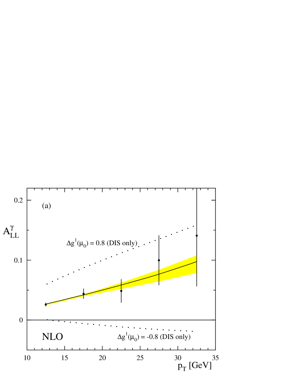
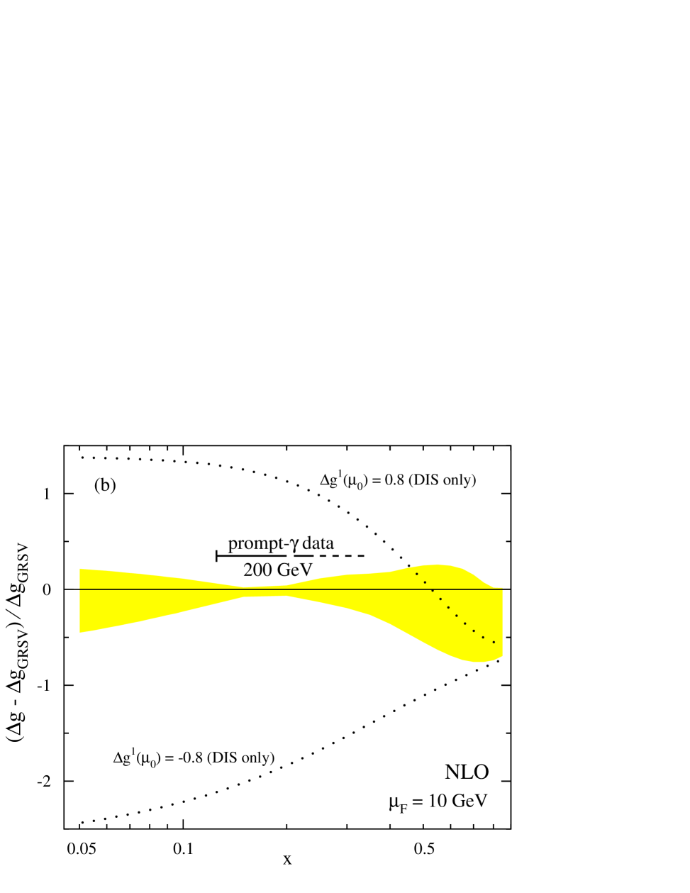
Figure 5: (a): Generated pseudo data for $A_{LL}^{\gamma}$ based on a calculation using the spin-dependent parton densities of [22] (solid line). The shaded band corresponds to the results of a large number of combined fits to DIS and $A_{LL}^{\gamma}$ data (see text). (b): Variations (shaded area) of the polarized gluon densities obtained in the combined fits, with respect to $\Delta g$ of [22], for $\mu_{F}=10\,\mathrm{GeV}$ (see text). Also shown are two extreme gluon densities (dotted lines) which give an excellent description of the polarized DIS data only.

Next, we perform a large number of fits to the full, DIS plus projected prompt photon, data set. We simultaneously fit all polarized parton densities, (anti)quarks and gluons, choosing the distributions of [22] as the input for the $\Delta q$, $\Delta\bar{q}$, but using randomly chosen values for the parameters in the ansatz for the polarized gluon distribution at the input scale $\mu_{0}$. Regarding the details of the evolution, we stay again within the setup of [22], but we choose a more flexible ansatz for the polarized gluon density,

$$\Delta g(x,\mu_{0})=N\,x^{\alpha}\,(1-x)^{\beta}\,(1+\gamma\,x)\;g(x,\mu_{0})\;,$$ (30)

which also allows for a zero in the $x$-shape of $\Delta g$. $g(x,\mu_{0})$ is the unpolarized gluon density [7] at the input scale of [22]. Note that the functional form for the polarized gluon density of [22], used for generating our pseudo-data, is included in Eq. (30) for $N=1.419,\,\alpha=1.43,\,\beta=0.15,\,\gamma=0$. Each fit takes only about $10\div 20$ minutes.

Ideally, thanks to the strong sensitivity of the prompt photon reaction to $\Delta g$, the gluon density in each fit should return close to the function we assumed when calculating the fictitious prompt photon “data”, in the region of $x$ probed by the data. Indeed, as shown in Fig. 5(b), this happens. The shaded band illustrates the deviations of the gluon densities obtained from the global fits to the “reference $\Delta g$” [22] used in generating the pseudo-data. It should be stressed that only those fits are admitted to the band that give a good simultaneous description of the DIS and $A_{LL}^{\gamma}$ data. Here we have tolerated a maximum increase of the total $\chi^{2}$ by up to four units from its minimum value. The shaded area in Fig. 5(a) shows the corresponding variations in $A_{LL}^{\gamma}$.

As is expected, all gluon densities are rather tightly constrained in the $x$-region dominantly probed by the prompt photon data. This is true in particular at $x\approx 0.15$, as a result of the most precise data point for $A_{LL}^{\gamma}$ at $p_{T}=12.5\,\mathrm{GeV}$. We note that one can also easily include the SIDIS data discussed in Section 3 into the global analysis without any significant increase of computing time for each fit. However, so far these data have no impact on our results. To illustrate our present ignorance of $\Delta g$, Fig. 5(b) shows also two extreme gluon densities with first moments $\Delta g^{1}(\mu_{0})=\pm 0.8$ (dotted lines), which are both in perfect agreement with all presently available DIS data. The corresponding predictions for $A_{LL}^{\gamma}$ for these two sets are given in Fig. 5(a). It should be noted that future measurements of $A_{LL}^{\gamma}$ at RHIC at $\sqrt{S}=500\,\mathrm{GeV}$ and for similar $p_{T}$ values of the prompt photon would further reduce the uncertainties on $\Delta g$ in the $x$-region between 0.05 and 0.1. Although our analysis still contains a certain bias by choosing only the framework of [22] for the fits as well as by our choice of what $\chi^{2}$ values are still tolerable, it clearly outlines the potential and importance of upcoming measurements of $A_{LL}^{\gamma}$ at RHIC for improving our understanding of the spin structure of the nucleon, in particular of its spin-dependent gluon density.

5 Conclusions

To conclude, we have presented and applied a powerful technique for implementing in a fast way, and without any approximations, higher-order calculations of partonic cross sections into global analyses of parton distribution functions. We have demonstrated that the approach works in practice for two examples: SIDIS and prompt photon production in $pp$ collisions. In the first case it was possible to perform the Mellin transform analytically and we have provided all necessary technical details for future analyses of polarized and unpolarized SIDIS data. For polarized prompt photon production we have presented a case study for a future global analysis based on fictitious data. The Mellin transform method is certainly applicable to any other reaction of interest, and it could equally well be an improvement also in any global analysis of unpolarized parton distributions.

References

-
[1]
European Muon Collaboration (EMC), J. Ashman et al.,
Phys. Lett. B206, 364 (1988);
Nucl. Phys. B328, 1 (1989);
for a recent review of the data on polarized deep-inelastic scattering, see: E. Hughes and R. Voss, Annu. Rev. Nucl. Part. Sci. 49, 303 (1999). -
[2]
D. Diakonov et al., Nucl. Phys.
B480, 341 (1996); Phys. Rev. D56, 4096 (1997);
M. Wakamatsu and T. Kubota, Phys. Rev. D60, 034020 (1999);
K. Goeke et al., Acta Phys. Polon. B32, 1201 (2001). -
[3]
R.S. Bhalerao, Phys. Lett. B380, 1 (1996);
B387, 881 (1996) (E); Nucl. Phys. A680, 62 (2000);
Phys. Rev. C63, 025208 (2001);
R.S. Bhalerao, N.G. Kelkar, and B. Ram, Phys. Lett. B476, 285 (2000);
R.J. Fries and A. Schäfer, Phys. Lett. B443, 40 (1998);
F.-G. Cao and A.I. Signal, Eur. Phys. J. C21, 105 (2001). - [4] M. Glück and E. Reya, Mod. Phys. Lett. A15, 883 (2000).
- [5] for a recent review of the RHIC spin physics program, see: G. Bunce, N. Saito, J. Soffer, and W. Vogelsang, Annu. Rev. Nucl. Part. Sci. 50, 525 (2000).
-
[6]
CTEQ Collaboration, H.L. Lai et al.,
Eur. Phys. J. C12, 375 (2000);
A.D. Martin, R.G. Roberts, W.J. Stirling, and R.S. Thorne, Eur. Phys. J. C4, 463 (1998). - [7] M. Glück, E. Reya, and A. Vogt, Eur. Phys. J. C5, 461 (1998).
- [8] C. Berger, D. Graudenz, M. Hampel, and A. Vogt, Z. Phys. C70, 77 (1996).
- [9] D.A. Kosower, Nucl. Phys. B520, 263 (1998).
- [10] Spin Muon Collaboration (SMC), B. Adeva et al., Phys. Lett. B420, 180 (1998).
- [11] HERMES Collaboration, K Ackerstaff et al., Phys. Lett. B464, 123 (1999).
-
[12]
S.B. Libby and G. Sterman, Phys. Rev. D18, 3252
(1978);
R.K. Ellis, H. Georgi, M. Machacek, H.D. Politzer, and G.G. Ross, Phys. Lett. 78B, 281 (1978); Nucl. Phys. B152, 285 (1979);
D. Amati, R. Petronzio, and G. Veneziano, Nucl. Phys. B140, 54 (1980); Nucl. Phys. B146, 29 (1978);
G. Curci, W. Furmanski, and R. Petronzio, Nucl. Phys. B175, 27 (1980);
J.C. Collins, D.E. Soper, and G. Sterman, Phys. Lett. B134, 263 (1984); Nucl. Phys. B261, 104 (1985);
J.C. Collins, Nucl. Phys. B394, 169 (1993). -
[13]
G. Altarelli and G. Parisi, Nucl. Phys. B126, 298
(1977);
Yu.L. Dokshitser, Sov. Phys. JETP 46, 641 (1977);
L.N. Lipatov, Sov. J. Nucl. Phys. 20, 95 (1975);
V.N. Gribov and L.N. Lipatov, Sov. J. Nucl. Phys. 15, 438 (1972). - [14] M. Glück, E. Reya, and A. Vogt, Z. Phys. C48, 471 (1990).
- [15] D. de Florian, M. Stratmann, and W. Vogelsang, Phys. Rev. D57, 5811 (1998).
-
[16]
D. de Florian, C.A. Garcia Canal,
and R. Sassot, Nucl. Phys. B470, 195 (1996);
D. de Florian et al., Phys. Lett. B389, 358 (1996). - [17] G. Altarelli, R.K. Ellis, G. Martinelli, and S.-Y. Pi, Nucl. Phys. B160, 301 (1979).
-
[18]
W. Furmanski and R. Petronzio,
Z. Phys. C11, 293 (1982);
P. Nason and B. Webber, Nucl. Phys. B421, 473 (1994); B480, 755(E) (1996). - [19] D. de Florian and R. Sassot, Phys. Rev. D62, 094025 (2000).
- [20] A.N. Sissakian, O.Yu. Shevchenko, and V.N. Samoilov, hep-ph/0010298.
- [21] S. Kretzer, Phys. Rev. D62, 054001 (2000).
- [22] M. Glück, E. Reya, M. Stratmann, and W. Vogelsang, Phys. Rev. D63, 094005 (2001).
-
[23]
A.P. Contogouris, B. Kamal, Z. Merebashvili, and
F.V. Tkachov, Phys. Lett. B304, 329 (1993);
Phys. Rev. D48, 4092 (1993);
A.P. Contogouris and Z. Merebashvili, Phys. Rev. D55, 2718 (1997);
L.E. Gordon and W. Vogelsang, Phys. Rev. D48, 3136 (1993); Phys. Rev. D49, 170 (1994);
S. Frixione and W. Vogelsang, Nucl. Phys. B568, 60 (2000). - [24] S. Frixione, Phys. Lett. B429, 369 (1998).