An example of resonance saturation at one loop

O. Catà and S. Peris

Grup de Física Teòrica and IFAE

Universitat Autònoma de Barcelona, 08193 Barcelona, Spain.

We argue that the large-Nc expansion of QCD can be used to treat a Lagrangian of resonances in a perturbative way. As an illustration of this we compute the $L_{10}$ coupling of the Chiral Lagrangian by integrating out resonance fields at one loop. Given a Lagrangian and a renormalization scheme, this is how in principle one can answer in a concrete and unambiguous manner questions such as at what scale resonance saturation takes place.

Ever since the early times of Vector Meson Dominance[1] there has been constant phenomenological evidence for the lowest vector and axial vector states to essentially saturate hadronic observables whenever their contribution is allowed by quantum number conservation. In the context of Chiral Perturbation Theory [2, 3] resonance saturation was suggested to generalize also to the scalar and pseudoscalar sectors[4], and indeed all the $O(p^{4})$ $L_{i}$ couplings were obtained by means of integrating out the appropriate resonance fields. However, this integration was carried out at tree level, i.e., the Lagrangian was effectively treated only as classical.

Specifically Ref. [4] made the choice to represent vector and axial-vector particles by antisymmetric tensor fields and wrote down a Lagrangian with $SU_{3}^{L}\times SU_{3}^{R}$-symmetric interactions of the form

$${\cal L}_{R} \!\!=\! -\frac{1}{2}{\sum_{R=V,A}}{\langle{\nabla}^{\lambda}R_{\lambda\mu}{\nabla}_{\nu}R^{\nu\mu}-\frac{1}{2}M_{R}^{2}R_{\mu\nu}R^{\mu\nu}}\rangle\,+\,\frac{1}{2}\,\langle\nabla^{\mu}S\nabla_{\mu}S-M_{S}^{2}S^{2}\rangle$$ (1)

$$+\,\frac{1}{2}\,\langle\partial^{\mu}S_{1}\partial_{\mu}S_{1}-M_{S_{1}}^{2}S_{1}^{2}\rangle\,+\,\frac{F_{\pi}^{2}}{4}\,{\langle D_{\mu}UD^{\mu}U^{\dagger}}\rangle$$

$$+\,\frac{F_{V}}{2\sqrt{2}}\,{\langle V_{\mu\nu}f_{+}^{\mu\nu}}\rangle\,+\,i\,\frac{G_{V}}{\sqrt{2}}\,{\langle V_{\mu\nu}u^{\mu}u^{\nu}}\rangle\,+\,\frac{F_{A}}{2\sqrt{2}}\,{\langle A_{\mu\nu}f_{-}^{\mu\nu}}\rangle$$

$$+\,c_{d}\,\langle Su_{\mu}u^{\mu}\rangle\,+\,\tilde{c}_{d}\,S_{1}\,\langle u_{\mu}u^{\mu}\rangle\,+\,L_{10}^{\mathcal{{}^{R}}}\,{\langle U^{\dagger}F_{R}^{\mu\nu}UF_{L\mu\nu}}\rangle\ ,$$

where $V,A,S$ and $S_{1}$ stand for the octet vector, axial-vector, scalar and singlet scalar resonance fields, respectively, and $U$ is the exponential of the Goldstone fields. Other terms appearing in the Lagrangian of Ref. [4] will be of no relevance for the discussion that follows and are not considered in Eq. (1).

As is well known the field representation is not unique and, for instance, in the case of spin-one particles different authors have chosen different representations to describe them (i.e. an antisymmetric tensor, Yang-Mills field, Hidden-Symmetry field, etc…[7, 8]). As a consequence of this, it was seen that ambiguities in physical observables may occur. In Ref. [6] these ambiguities were resolved by imposing short-distance matching onto the QCD Operator Product Expansion of certain Green’s functions. As a matter of fact, it was shown later on in Ref. [9] that all the above choices in the representation were actually field redefinitions of the particular Lagrangian of Eq. (1).

Let us take the case of $L_{10}$ as an example. Integrating the vector and axial-vector fields in the Lagrangian (1) at tree level leads to the low-energy chiral Lagrangian of Eq. (3) (see below) with equations relating couplings below and above threshold, such as

$$L_{10}(\mu)=\frac{F_{A}^{2}}{4M_{A}^{2}}-\frac{F_{V}^{2}}{4M_{V}^{2}}+L_{10}^{\mathcal{R}}(\mu)\ .$$ (2)

Here $L_{10}(\mu)$ stands for the $O(p^{4})$ coupling in the low-energy Lagrangian after the V and A resonance fields have been integrated out, i.e.

$${\cal L}_{\chi\rm{PT}}=\frac{F_{\pi}^{2}}{4}{\langle D_{\mu}UD^{\mu}U^{\dagger}}\rangle\,\,+\,\,L_{10}\ {\langle U^{\dagger}F_{R}^{\mu\nu}UF_{L\mu\nu}}\rangle+\mathcal{O}(L_{i},i=1,\ldots,9)\ ,$$ (3)

whereas $L_{10}^{\mathcal{R}}(\mu)$ is the akin coupling, but at the level of the resonance Lagrangian (1). The other couplings $L_{1-9}$ complete the list at $\mathcal{O}(p^{4})$[3]. The statement of resonance saturation is then tantamount to the equation

$$L_{10}^{\mathcal{R}}(\mu)=0\ ,$$ (4)

and expresses the fact that the whole low-energy coupling $L_{10}$ is directly “produced” in the process of integrating the resonance field.

The result of Eq. (4) is actually field representation dependent and is true only in the antisymmetric tensor formulation, i.e. for the Lagrangian in Eq. (1). Other formulations (i.e. Yang-Mills, Hidden-Symmetry,etc…) may have non-zero values of $L_{10}^{\mathcal{R}}(\mu)$ to balance the different contribution from the direct integration of the resonance fields to finally produce the same value for $L_{10}(\mu)$, as it is produced by the field redefinition connecting the different formulations[9]. Alternatively, this may also be seen as a consequence of certain matching conditions to QCD at short distances[6]. Therefore, although at tree level $L_{10}(\mu)$ is always given by the same combination of resonance parameters regardless of the formulation, it is in the antisymmetric tensor representation that it originates solely from the interactions of the resonance fields in the Effective Lagrangian, with the matching to QCD at short distances appearing as automatic.

Since the left hand side of Eq. (4) in general obeys a nontrivial Renormalization Group equation, i.e. it is $\mu$ dependent, while the right hand side is a constant, this equation has to be supplied with the prescription of some value for $\mu$ at which it is supposed to be valid, which we shall call $\mu^{*}$. Notice that if it happens that $L^{\mathcal{R}}_{i}(\mu^{*})=0$ ($i=1,...,10$), for a certain $\mu^{*}$ of the order of a resonance mass, then one can use this as a boundary condition to predict all the low-energy couplings $L_{i}(\mu)$ of the chiral Lagrangian at scales $\mu\leq\mu^{*}$. The scale $\mu^{*}$ can then be given the meaning of a threshold between the low-energy chiral Lagrangian and the resonance Lagrangian that would take over at higher energies.

In Ref. [4, 6] it was argued that the natural choice is $\mu^{*}=M_{V}$; and the coupling $L_{10}^{\mathcal{R}}(M_{V})$ was omitted from the resonance Lagrangian (1) in accord with Eq. (4). With this prescription for $\mu^{*}$ Eq. (2) leads to a prediction for $L_{10}(M_{V})$ in terms of known resonance masses and decay constants. Similar results were also obtained for all the rest of the $L_{i},i=1,\dots,9$ with remarkable overall agreement with the experimental determinations[4, 10].

However the former agreement, although clearly important, is necessarily only of a qualitative nature. No attempt is made at defining the underlying QCD approximation that is being used and, as a consequence, it is not clear how to systematically improve it. For instance the prescription $\mu=M_{V}$ to effect resonance saturation may indeed be natural but only as long as one is prepared not to distinguish between the two scales $M_{V}=0.77\textrm{GeV}$ and $M_{A}=1.25\textrm{GeV}$, both of which in turn must be identified with something like $\Lambda_{\chi}\sim 1\textrm{GeV}\gg M_{K,\pi}$. At some level of accuracy, however, one may eventually want to distinguish between $M_{V}$ and $M_{A}$; after all $M_{A}-M_{V}$ is actually larger than $M_{V}-M_{K}$, for instance. Furthermore, it is not clear from just a tree-level integration whether the Lagrangian (1) actually saturates the $L_{i}$’s at $\mu=M_{V}$, since the scale $\mu$ first appears at one loop.

In Ref. [11] it was realized that the above scheme of resonance saturation can be best understood as an approximation to large-$N_{c}$ QCD[12], which was called Lowest Meson Dominance. This is the approximation in which, out of the (in principle) infinite set of resonances, only the lowest one is kept in each channel. We remark that this approximation can be improved upon since, in principle, more resonances may be added whose couplings and masses can be fixed by matching to higher terms in the Operator Product Expansion at short distances. Adopting the large-$N_{c}$ expansion right from the start justifies, for instance, the tree-level integration of the resonance fields employed in Ref. [4, 6] since this is precisely the leading contribution at large $N_{c}$. This also tells you that it makes no sense to be more precise on the value of the scale $\mu$ at which one is doing the matching unless one goes to the next order in the large-$N_{c}$ expansion, as the difference between two scales $\mu$ and $\mu^{\prime}$ necessarily yields a contribution of subleading order in $1/N_{c}$. Consequently, Eq. (2) is a statement at leading order in the $1/N_{c}$ expansion in which the $\mu$ dependence of both sides remains, strictly speaking, ill-defined until next-to-leading (i.e. quantum) effects are computed. This new point of view of resonance saturation as an approximation to large-$N_{c}$ QCD is now being studied and successfully applied to many different problems in hadron physics[13].

In this letter we shall adopt large-$N_{c}$ as our underlying expansion and (1) as our resonance Lagrangian. We merely wish to illustrate the point that, as a consequence of the large-$N_{c}$ expansion, it makes sense to compute quantum corrections with a resonance Lagrangian and ask, for instance, the question of at which scale $\mu$ resonance saturation takes place, if it does at all. Specifically we shall consider $1/N_{c}$ quantum effects that give rise to a nontrivial $\mu$ dependence in Eq. (2).

In order to make this explicit we shall take the Lagrangian (1) as our starting point. This we do although this Lagrangian is probably too simple to satisfy the short-distance constraints of QCD at next-to-leading order in the large-$N_{c}$ expansion, even in the particular case of the $\Pi_{LR}$ function which will be the relevant one here. Therefore, in this sense, our analysis cannot be considered fully realistic for QCD. Notice that Ref. [6] showed the good matching of this Lagrangian to QCD only at leading order in $1/N_{c}$ and, even then, only for certain Green’s functions. Further interesting studies can be found in [14] and, in particular, in [15]. It is obvious that determining the resonance Lagrangian that satisfies the short distance constraints at the next-to-leading order in $1/N_{c}$, even only in all the Green’s functions studied up to now, is an extremely arduous task. Therefore, here we will have to content ourselves with a much more modest goal.

In this letter we shall restrict ourselves to the particular case of the $L_{10}$ coupling. This we do because this coupling is defined in terms of a two-point Green’s function in QCD, which makes life simpler. At the same time both vector and axial-vector particles affect $L_{10}$, which makes it a sensitive probe for whether $M_{V}$ or $M_{A}$ (or neither one) should be the relevant scale driving the statement of resonance saturation, Eq. (4). In other words, we want to find out if the Lagrangian of Eq. (1) is at least capable of reproducing the right value for $L_{10}$ at some scale $\mu^{*}$, once quantum corrections are taken into account and whether this scale $\mu^{*}$ indeed coincides with $M_{V}$ or not. This will entail a calculation with the Lagrangian of Eq. (1) and resonances running around in loops. It is then that the large-$N_{c}$ counting becomes important. Resonances are not amenable to a chiral counting like Goldstone bosons are and, were it not for the large-$N_{c}$ expansion, there would be no obvious small parameter with which to do perturbation theory . This is the main advantage of the large-$N_{c}$ expansion for the purposes of this work: QCD in the limit $N_{c}\rightarrow\infty$ is a theory of free, noninteracting hadrons and, consequently, interactions among them are modulated by increasing inverse powers of $N_{c}$. In other words, there is a “small” coupling governing hadron interactions (no matter at which energy) and, with it, a sense in which loops are smaller than the tree level.

One of the consequences of using the large-$N_{c}$ expansion is that now we have to enlarge the flavor symmetry in the Lagrangian of Eq. (1) from $SU_{3}^{L}\times SU_{3}^{R}$ to $U_{3}^{L}\times U_{3}^{R}$ [17] to incorporate the $\eta_{1}$. This can easily be done by means of the replacement

$$U\longrightarrow Ue^{-i\frac{\sqrt{2}}{\sqrt{3}}\frac{\eta_{1}}{F_{\pi}}}\ .$$ (5)

To begin, let us define the $\Pi_{LR}$ function ($Q^{2}\equiv-q^{2}\geq 0$ for $q^{2}$ space–like) as

$$\Pi_{LR}^{\mu\nu}(q)\delta_{ab}=2i\int d^{4}x\,e^{iq\cdot x}\langle 0|\mbox{\rm T}\left(L^{\mu}_{a}(x)R^{\nu}_{b}(0)^{\dagger}\right)|0\rangle\,,$$ (6)

with color-singlet currents

$$R_{a}^{\mu}\left(L_{a}^{\mu}\right)=\bar{q}(x)\gamma^{\mu}\ \frac{\lambda_{a}}{\sqrt{2}}\ \frac{(1\pm\gamma_{5})}{2}\ q(x)\,,$$ (7)

where $q=u,d,s$ and $\lambda_{a}$ are Gell-Mann matrices in flavor space.

In the chiral limit, $m_{u,d,s}\rightarrow 0$  , this correlation function has only a transverse component,

$$\Pi_{LR}^{\mu\nu}(Q^{2})=(q^{\mu}q^{\nu}-g^{\mu\nu}q^{2})\Pi_{LR}(Q^{2})\,.$$ (8)

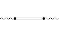
Figure 1: Tree-level contribution to $\Pi(q^{2})_{LR}$ from the Lagrangian in Eq.(1). The double line stands for the $V$ and $A$ propagators; the dot for the insertion of $L_{10}^{\mathcal{R}}$.

Figure 2: Tree-level contribution from the Lagrangian in Eq.(3), but now the dot stands for the insertion of $L_{10}$.

At low energy Green’s functions in general, and $\Pi_{LR}(Q^{2})$ in particular, should be equal in the two theories with Lagrangians (1) and (3). For the case of $L_{10}$ that we are here concerned with, it is immediately seen that the result in Eq. (2) is the matching condition that results (at tree level) from demanding that the “slope” in $Q^{2}$, i.e. the combination

$$-\frac{1}{4}\frac{d}{dQ^{2}}\left\{Q^{2}\Pi_{LR}(Q^{2})\right\}_{Q^{2}=0}\ ,$$ (9)

be equal when computed both with the Lagrangian in Eq. (1) and with that in Eq. (3). This is just given by the diagrams in Figs. 1 and 2 .

Figure 3: One-loop contribution to $\Pi_{LR}$ from the Lagrangian in Eq.(3). The dotted line stands for the Goldstone bosons included in the matrix $U$.

We now move to the contribution at one loop. Firstly, let us consider the contribution to $\Pi_{LR}$ stemming from the Lagrangian in Eq. (3). The result is given by the diagram depicted in Fig. 3 plus again the direct contribution from the coupling $L_{10}$ in Fig. 2. As a renormalization scheme we shall use throughout the particular $d$-dimensional $\overline{\textrm{MS}}$ variant used in [3] in which, e.g., $L_{10}$ renormalizes according to

$$L^{\mathrm{bare}}_{10}=L_{10}(\mu)-\frac{1}{4}\frac{\mu^{d-4}}{(4\pi)^{2}}\left\{\frac{1}{d-4}-\frac{1}{2}\left(\log 4\pi+\Gamma^{\prime}(1)+1\right)\right\}\ .$$ (10)

Then one obtains the well-known result

$$\Pi_{LR}(Q^{2})=4L_{10}(\mu)-\frac{1}{32\pi^{2}}\left(\frac{5}{3}-\log{\frac{Q^{2}}{\mu^{2}}}\right)\ ,$$ (11)

where $L_{10}(\mu)$ is the renormalized coupling in $\overline{\textrm{MS}}$. Since $\Pi_{LR}$ is $\mu$ independent this equation implies the usual renormalization group equation for $L_{10}(\mu)$.

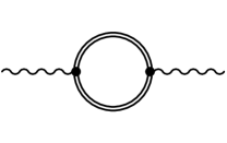
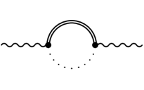
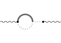
Figure 4: One-loop contribution to $\Pi_{LR}$ from the Lagrangian of resonances in Eq.(1). Double lines stand for resonance propagators. Dotted lines stand for Goldstone propagators.

The diagrams giving the resonance contribution to $\Pi_{LR}$ at one loop are depicted in Fig. 4. Adding all the one-loop contributions in Fig. 4 to the tree-level of Fig. 1 and to the one-loop of Goldstones in Fig. 3 one gets the total contribution to $\Pi_{LR}$ from the Lagrangian (1). Equating this expression to that in Eq. (11) one verifies that the Goldstone loop cancels out in the matching (as it should) and one finally obtains for $L_{10}$

$$4\ L_{10}(\mu) = \frac{F_{A}^{2}}{M_{A}^{2}}-\frac{F_{V}^{2}}{M_{V}^{2}}$$ (12)

$$-\frac{3}{2}\frac{F_{A}^{2}}{f_{\pi}^{2}}\frac{1}{(4\pi)^{2}}\left(\frac{1}{2}-\log\frac{M_{A}^{2}}{\mu^{2}}\right)+\frac{3}{2}\frac{F_{V}^{2}}{f_{\pi}^{2}}\frac{1}{(4\pi)^{2}}\left(\frac{1}{2}-\log\frac{M_{V}^{2}}{\mu^{2}}\right)$$

$$-\frac{5}{(4\pi)^{2}}\frac{G_{V}^{2}}{f_{\pi}^{2}}\left(-\frac{17}{30}-\log\frac{M_{V}^{2}}{\mu^{2}}\right)$$

$$+\frac{3}{2}\frac{1}{(4\pi)^{2}}\left(-\frac{1}{3}-\log\frac{M_{A}^{2}}{\mu^{2}}\right)+\frac{3}{2}\frac{1}{(4\pi)^{2}}\left(-\frac{1}{3}-\log\frac{M_{V}^{2}}{\mu^{2}}\right)$$

$$-\frac{4}{3}\left(\frac{{\tilde{c}}_{d}}{f_{\pi}}\right)^{2}\frac{1}{(4\pi)^{2}}\left(\frac{1}{6}+\log\frac{M_{S_{1}}^{2}}{\mu^{2}}\right)-\frac{10}{9}\left(\frac{c_{d}}{f_{\pi}}\right)^{2}\frac{1}{(4\pi)^{2}}\left(\frac{1}{6}+\log\frac{M_{S}^{2}}{\mu^{2}}\right)$$

$$+\frac{1}{2}\frac{1}{(4\pi)^{2}}\left(1+\log\frac{M_{S}^{2}}{\mu^{2}}\right)-\frac{4}{9}\left(\frac{c_{d}}{f_{\pi}}\right)^{2}\frac{1}{(4\pi)^{2}}\Bigg{[}\frac{1}{6}+\log\frac{M_{S}^{2}}{\mu^{2}}$$

$$+2B+2B^{2}-(2B^{3}+3B^{2})\log\frac{M_{S}^{2}}{M_{\eta_{1}}^{2}}\Bigg{]}$$

$$+4\ L_{10}^{\mathcal{R}}(\mu)\ ,$$

where we have defined $B=M_{\eta_{1}}^{2}/(M_{S}^{2}-M_{\eta_{1}}^{2})$. As to the large-$N_{c}$ counting, we shall consider $L_{10}^{\mathcal{R}}(\mu)$ of $\mathcal{O}(1)$. Since $F_{V,A}^{2},G_{V}^{2},c_{d}^{2}$ and $\tilde{c}_{d}^{2}$ are $\mathcal{O}(N_{c})$, while the resonance masses are $\mathcal{O}(1)$, the tree-level contribution above is $\mathcal{O}(N_{c})$ while the one-loop one is $\mathcal{O}(1)$, as it should.

\psfrag{m}{$\mu$}\includegraphics[width=325.215pt]{L10.eps}

Figure 5: This figure shows the curve obtained for $L_{10}(\mu)$ in Eq. (12) as a function of $\mu$ (in MeV) under the condition $L^{\mathcal{R}}_{10}(\mu)=0$ (solid curve). The dashed curve is the running of $L_{10}(\mu)$ according to Eq. (15). For comparison we also show the tree level contribution to $L_{10}(\mu)$ (first line in Eq. (12)) as dot-dashed lines. All three curves have been normalized to the central value of the tree level resonance contribution.

In the work of Refs. [6, 11] it was found that the tree-level matching (i.e. leading at large $N_{c}$) of the Lagrangian (1) to the short-distance behavior of certain Green’s functions in QCD led to the constraints $F_{A}=f_{\pi}$, $F_{V}=\sqrt{2}f_{\pi}$, $G_{V}=f_{\pi}/\sqrt{2}$, $M_{A}=\sqrt{2}M_{V}$ and $M_{V}=4\pi f_{\pi}(\sqrt{6}/5)^{1/2}$. Consequently these are constraints among the parameters in the Lagrangian (1). These are not in principle the same thing as the physical mass (defined as the pole in the propagator) and physical decay constant (defined,e.g., through the width), but it is precisely the parameters in the Lagrangian and not the physical ones what appears in Eq. (12). This is why the first term in Eq. (12), namely

$$\frac{F_{A}^{2}}{M_{A}^{2}}-\frac{F_{V}^{2}}{M_{V}^{2}}\ ,$$ (13)

is in fact predicted to be

$$-\frac{15}{32\pi^{2}\sqrt{6}}\$$ (14)

in this equation. In passing one also sees that the $\log M_{A}$ dependence cancels out in Eq. (12). It is intriguing to entertain the idea that the above relations between masses and decay constants could be a consequence of a higher symmetry of the planar graphs of QCD.

Looking at (12), one sees clearly that knowledge of $L^{\mathcal{R}}_{10}(\mu)$ immediately translates into a prediction for $L_{10}(\mu)$. Using the above constraints and $f_{\pi}=87\pm 3.5$ MeV (chiral limit) together with the phenomenological values $c_{d}^{2}=\tilde{c}_{d}^{2}/3=1024$ MeV² and $M_{S}=M_{S_{1}}=983$ MeV[4], one can now take Eq. (12) and compare it to the expression for the running of $L_{10}$[3]:

$$L_{10}(\mu)=L_{10}(M_{\rho})-\frac{1}{64\pi^{2}}\log\frac{M_{\rho}}{\mu}\ ,$$ (15)

where $L_{10}(M_{\rho})=(-5.13\pm 0.19)\times 10^{-3}$ [18]. This comparison is made in Fig. 5. In this figure one can see how the Lagrangian (1) is actually able to produce the right experimental value for $L_{10}(\mu)$, but at a value for $\mu$ which is much lower than what was expected in Ref. [4]. This happens at $\mu^{*}\sim 380$ MeV where, as it turns out, the condition of resonance saturation is fulfilled, namely $L^{\mathcal{R}}_{10}(\mu^{*})=0$. Notice that, as Fig. 5 shows, at the scale $\mu^{*}$ the one-loop radiative corrections are $\sim 30\%$ of the tree level, so one is reasonably within the perturbative regime expected for the $1/N_{c}$ expansion. In fact, at $\mu\sim 490$ MeV the one-loop contribution vanishes altogether. On the other hand, at higher scales the one-loop corrections quickly grow and one finds, e.g., a $\sim 60\%$ reduction relative to the tree level at $\mu\sim 800\ \mathrm{MeV}\sim M_{V}$; with even larger corrections the higher the scale $\mu$. In other words, at this scale $L^{\mathcal{R}}_{10}$ must be $\sim 60\%$ of the tree level and clearly different from zero for Eq. (12) to be satisfied. Therefore resonance saturation for the Lagrangian (1) with the renormalization scheme (10) does not take place at the large values of $\mu$, namely $\mu\approx\Lambda_{\chi}\sim 1$GeV, where one would like the resonance Lagrangian (1) to take over from the low-energy chiral Lagrangian (3).

Perhaps some discussion on the meaning of $L^{\mathcal{R}}_{10}(\mu^{*})=0$ is now in order. As a matter of fact, only from the knowledge of the value of $\mu^{*}$ which satisfies this condition one does not learn much. For one thing $L^{\mathcal{R}}_{10}(\mu)=0$ is a renormalization scheme dependent condition on $\mu^{*}$ (in our case the scheme was given in Eq. (10)) and therefore, strictly speaking, $\mu^{*}$ can be shifted by a change in the renormalization scheme . Even with this caveat in mind, the low value of $\mu^{*}$ obtained in Eq. (12) makes one suspect the Lagrangian (1), if only because one already knows that (1) has several drawbacks, like e.g. the wrong short-distance behavior of certain Green’s functions due to the lack of a $\pi\rho\mathrm{a_{1}}$ coupling; just to mention one of them [14]. Clearly such a coupling plays no role at tree level in the determination of the $L_{i}$’s whereas, in principle, it will contribute at one loop. See also Ref. [15] for some other related limitations of this resonance Lagrangian.

In our view the scale $\mu^{*}$ is reminiscent of, for instance, the scale $M_{X}$ of gauge coupling unification in GUTs[20]. In fact, more physically meaningful than the value of $\mu^{*}$ itself are equations such as, e.g., $L^{\mathcal{R}}_{i}(\mu^{*})=0$ (for all $i=1,...,10$), since they lead to relations among the $L_{i}(\mu)$ at $\mu=\mu^{*}$ and therefore at all $\mu$. They can be used as a guide in the search for a more predictive resonance model. In this context one expects that even heavier resonances than those in the Lagrangian (1) are the ones which give rise to the couplings $L^{\mathcal{R}}_{i}(\mu)$ upon integration. Again we find in the framework of GUTs equations like $\alpha_{\mathrm{SU_{3}}}(M_{X})=\alpha_{\mathrm{SU_{2}}}(M_{X})=\alpha_{\mathrm{U_{1}}}(M_{X})$, which are a good example of this type of relations.

A particularly interesting situation for its high predictive power is what we could call the “extreme” version of resonance saturation. This is when $L^{\mathcal{R}}_{i}(\mu)=0$ (for all $i=1,...,10$) and for all $\mu$. In fact, just as $L_{10}(\mu)$ is obtained through a matching condition on the $\Pi_{LR}$ function which is an order parameter of spontaneous chiral symmetry breaking, so are all the other $L_{i}(\mu)$ obtained through corresponding matching conditions on certain QCD Green’s functions $\mathcal{G}$ which, because they are also order parameters, vanish in the chiral limit to all orders. This implies that all the $\mathcal{G}$’s have a finite and smooth short-distance behavior. It is conceivable, and in our opinion theoretically very appealing, that this finite ultraviolet behavior be realized at the level of the resonance Lagrangian. Restricted to the former Green’s functions $\mathcal{G}$, the resonance Lagrangian would then behave almost like renormalizable and would predict, upon integration of the resonance fields, all the $L_{i}(\mu)$ as a function of the resonance masses and couplings. Clearly, we believe, this is the picture which gets closest to the spirit of the work in Ref. [4]. A (surely oversimplified) sketch of the answer for $L_{10}(\mu)$ in this picture could have been

$$L_{10}(\mu)=-\ \frac{1}{4}\left(\frac{15}{32\pi^{2}\sqrt{6}}\right)-\frac{1}{64\pi^{2}}\log\frac{\Lambda_{\chi}}{\mu}\ ,$$ (16)

with $\Lambda_{\chi}$ a function of resonance masses and parameters and $\Lambda_{\chi}\simeq 800$ MeV. We remark that the coefficient in front of the logarithm should be the same as that in Eq. (15) . However, we have shown that the resonance interactions in the Lagrangian (1) do not produce this type of answer. The reason why our Eq. (12) is incompatible with the running of $L_{10}(\mu)$ in Eq. (15) and the condition $L^{\mathcal{R}}_{10}(\mu)=0,\forall\mu$, is because the resonance interactions in (1) do not produce a finite (i.e. $\mu$ independent) $\Pi_{LR}$ function. This is not to be unexpected as (1) lacks the right short-distance properties it should have[14, 15]. The dynamical challenge clearly will be to incorporate all these short-distance properties in a resonance Lagrangian which becomes more ultraviolet convergent and yields finite answers for all the above mentioned Green’s functions $\mathcal{G}$; consequently predicting all the $L_{i}(\mu)$ in this manner.

To conclude, we hope to have illustrated how one could use large-$N_{c}$ in the context of a resonance Lagrangian to test in a well-defined way the idea of resonance saturation at the quantum level. Although our resonance Lagrangian (1) cannot be considered fully realistic, it should be clear that a similar analysis to the one presented here could be performed should a more complete resonance Lagrangian of QCD be available. In this sense the present analysis is complementary to that of Ref. [15] in the quest for a resonance Lagrangian capable of pushing to higher energies the range of validity of the description of QCD in terms of meson degrees of freedom.

We thank G. Ecker, M. Knecht, J. Portoles and E. de Rafael for discussions and reading the manuscript. This work is supported by CICYT-AEN99-0766 and by TMR, EC-Contract No. ERBFMRX-CT980169 (EURODA$\phi$NE).

References

- [1] See for instance J.J. Sakurai, ”Currents and Mesons”, The Univ. of Chicago Press, 1969.
- [2] S. Weinberg, PhysicaA 96 (1979) 327.
- [3] J. Gasser and H. Leutwyler, Nucl. Phys. B 250 (1985) 465.
- [4] G. Ecker, J. Gasser, A. Pich and E. de Rafael, Nucl. Phys. B 321 (1989) 311.
- [5] J. F. Donoghue, C. Ramirez and G. Valencia, Phys. Rev. D 39 (1989) 1947.
- [6] G. Ecker, J. Gasser, H. Leutwyler, A. Pich and E. de Rafael, Phys. Lett. B 223 (1989) 425.
- [7] M. Bando, T. Kugo and K. Yamawaki, Phys. Rept. 164 (1988) 217.
- [8] U. G. Meissner, Phys. Rept. 161 (1988) 213.
- [9] J. Bijnens and E. Pallante, Mod. Phys. Lett. A 11 (1996) 1069 [hep-ph/9510338].
- [10] G. Amoros, J. Bijnens and P. Talavera, Nucl. Phys. B 585 (2000) 293 [Erratum-ibid. B 598 (2000) 293] [hep-ph/0003258]. See also M. Knecht and A. Nyffeler, hep-ph/0106034; B. Ananthanarayan, P. Buttiker and B. Moussallam, hep-ph/0106230.
- [11] S. Peris, M. Perrottet and E. de Rafael, JHEP9805 (1998) 011 [hep-ph/9805442]; M. F. Golterman and S. Peris, Phys. Rev. D 61 (2000) 034018 [hep-ph/9908252].
- [12] G. ’t Hooft, Nucl. Phys. B 72 (1974) 461; E. Witten, Nucl. Phys. B 160 (1979) 57.
- [13] M. Knecht, S. Peris and E. de Rafael, Phys. Lett. B 508 (2001) 117 [hep-ph/0102017]; M. Golterman and S. Peris, JHEP0101 (2001) 028 [hep-ph/0101098]; S. Peris, Nucl. Phys. Proc. Suppl. 96 (2001) 346 [Erratum hep-ph/0010162]; S. Peris, B. Phily and E. de Rafael, Phys. Rev. Lett. 86 (2001) 14 [hep-ph/0007338]; S. Peris and E. de Rafael, Phys. Lett. B 490 (2000) 213 [Erratum hep-ph/0006146]; M. Knecht, S. Peris and E. de Rafael, Nucl. Phys. Proc. Suppl. 86 (2000) 279 [hep-ph/9910396]; M. Knecht, S. Peris, M. Perrottet and E. de Rafael, Phys. Rev. Lett. 83 (1999) 5230 [hep-ph/9908283]; M. Knecht, S. Peris and E. de Rafael, Phys. Lett. B 443 (1998) 255 [hep-ph/9809594]; M. Knecht and E. de Rafael, Phys. Lett. B 424 (1998) 335 [hep-ph/9712457].
- [14] B. Moussallam, Nucl. Phys. B 504 (1997) 381 [hep-ph/9701400].
- [15] M. Knecht and A. Nyffeler, hep-ph/0106034.
- [16] E. Jenkins, A. V. Manohar and M. B. Wise, Phys. Rev. Lett. 75 (1995) 2272 [hep-ph/9506356].
- [17] E. Witten, Nucl. Phys. B 156 (1979) 269.
- [18] M. Davier, L. Girlanda, A. Hocker and J. Stern, Phys. Rev. D 58 (1998) 096014 [hep-ph/9802447].
- [19] See, e.g., G. Rodrigo and A. Santamaria, Phys. Lett. B 313 (1993) 441 [hep-ph/9305305];
- [20] See, e.g., L. Hall, Nucl. Phys. B 178 (1981) 75.