Assisted inflation via tachyon condensation

Abstract

In this paper we propose a new mechanism of inflating the Universe with non-BPS $D4$ branes which decay into stable $D3$ branes via tachyon condensation. In a single brane scenario the tachyon potential is very steep and unable to support inflation. However if the universe lives in a stack of branes produced by a set of non-interacting unstable $\tilde{D4}$ branes, then the associated set of tachyons may drive inflation along our $3$ spatial dimensions. After tachyon condensation the Universe is imagined to be filled with a set of parallel stable $D3$ branes. We study the scalar density perturbations and reheating within this setup.

]

I Introduction

Inflation [1] is perhaps the only known mechanism which can dynamically solve the flatness and the horizon problem of the Universe. The inflating field can also produce the density perturbations causally to match the startling observation made by the COBE satellite. The observation has measured the amplitude of the density perturbations in one part in $10^{5}$ with a slightly tilted spectrum [2]. It is this result which has boosted the hope that the coming generation satellite experiments might be able to constrain or possibly rule out some of the models. It is a theoretical and experimental challenge to find an exact shape of the potential and lacking this leads to more than a dozen viable inflationary models with some common features.

The moduli of string theory might provide us a natural candidate as an inflaton [3]. However, as a zero mode, moduli lacks potential with a stable minimum. It is not clear at the moment how non-perturbative effects would generate a potential for them and what could be the appropriate scale for inflation [4]. The moduli also accompanies a host of problems for cosmology because of their Planck mass suppressed couplings to the matter fields [5]. On the other hand string theory also provides various solitonic states in the non-perturbative spectrum. These solitonic states are strong-weak (S-duality) coupling partners of the states in the perturbative spectrum of the dual string theory. These states are known as Dp branes [6], where the open strings end on a hypersurface with $p$-spatial and one time-like dimension. These objects couple to gauge fields (coming from the RR sector) of rank $(p+1)$, where $p=-1,0,1,2,..,9$, and, $p$ is odd (even) for Type IIB (A) theory. These branes are known as BPS branes and are stable under variation of the string coupling. On the contrary, string theory also admits non-BPS Dp-branes (also labeled as $\tilde{Dp}$) for odd (even) $p$ in Type IIA (B) [7]. Generically these are unstable because of the presence of tachyonic state(s) in their world volume, though in some cases they may become stable. For the stable non-BPS branes the tachyonic states are projected out of the spectrum by orbifolding, or, orientifolding procedure [8]. They can be the lightest states in the spectrum carrying some conserved charges and hence cannot decay to anything else and thus are stable objects. For unstable non-BPS branes where there are tachyonic states living on the world volume of the brane the tachyon can condense over a kink yielding a brane with one dimension less [9]. For an example, let us consider a coincident pair of Dp-brane and anti-Dp-brane (with opposite RR charge and both independently being BPS). There is a complex tachyon field $T$ living on the world volume of this system. If we integrate out all the massive modes on the world volume except the tachyon, we obtain the tachyon potential $V(T)$ with $T=0$ being the maximum of the potential. Since, there is $U(1)\times U(1)$ gauge field living on the world volume of the brane-antibrane system, the tachyon picks up a phase under the gauge transformation of each of this $U(1)$, and finally the potential becomes a function of $|T|$. Thus, the minimum of the potential occurs at $T=T_{0}e^{i\theta}$ for some fixed $T_{0}$ but arbitrary $\theta$. According to the conjecture of Sen, at the minimum the sum of the tension of the brane and the anti-brane, and, the (negative) potential energy of the tachyon should be exactly zero. Thus, the tachyonic ground state at the minimum of the potential is indistinguishable from the vacuum. However, instead of considering the tachyonic ground state if we consider a tachyonic kink solution, one finds that the energy density is concentrated around a $(p-1)$ dimensional subspace and the solution describes a $(p-1)$-dimensional brane. However, this solution is not stable since the manifold describing the minimum of the tachyon potential is a circle. This is also consistent with the identification of the kink solution with a non-BPS brane of a string theory since it has a tachyonic mode living on its own world volume.

One can continue one step further by considering a non-BPS $p$-brane. The tachyon which lives on its world volume is a real tachyon. But there is a $Z_{2}$ symmetry on the world volume of this non-BPS brane under which the tachyon changes sign. Therefore, in this case, $\pm T_{0}$ becomes the minimum of the tachyon potential obtained by integrating out other massive modes and at the minimum of the potential the sum of the (negative) potential and the tension of the non-BPS brane vanishes. Like in the previous case, instead of the tachyonic ground state if we consider the tachyonic kink solution, the configuration actually describes a $(p-1)$-brane. However, the kink solution now is a stable solution, since the manifold describing the minimum of the tachyon potential consists of just two disconnected points $\pm T_{0}$ (related by a $Z_{2}$-symmetry). This configuration, thus is identified with a BPS $(p-1)$-brane of the theory.

The tachyonic potential, either on the world volume of the brane-antibrane system, or, on the world volume of the non-BPS brane is not calculable explicitly. However, an approximate nature of the potential with the properties as mentioned above has been conjectured and such a potential is well supported by string field theory calculations. We will assume such expressions for the tachyon potential on either a single non-BPS $D4$-brane or a system of non coincident $\tilde{D4}$-branes of Type IIB string theory and test whether tachyons could play any role in the early Universe.

Recently, there has been a spate of interesting ideas which propose the Universe as a D3 brane, or a stack of D3 branes on top of each other, where ultimately the Standard Model fields are trapped [10]. These new ideas come up with a host of new cosmological issues and several new ideas have been discussed, such as inflationary [11, 12, 13, 14, 15, 16], and non-inflationary scenarios [17, 18]. One of the common feature these models possess is to inflate the brane by altering inter-brane separation. From the four dimensional point of view this corresponds to a scalar field known as radion. Fluctuations in the radion field can also lead to the density perturbations observed by the COBE satellite and eventually the radion couplings to matter fields lead to its decay to produce large entropy. A completely new possibility may arise where inflation does not depend on the relative motion of the branes. Inflation now depends on the intrinsic properties of an unstable $\tilde{D}4$ brane which decays into a stable $D3$ brane. This may happen due to the dynamics of a zero mode of the tachyon field. Usually, the tachyon potential is quite steep, and, can not support slow-rolling of the tachyon field. Instead, the tachyon rolls down extremely fast. However, under certain circumstances it is indeed possible to construct a model where more than one tachyon fields are present in the spectrum which might alleviate this situation. This goes under the notion of assisted inflation discussed in Refs. [19, 20]. We show that about ten of such tachyonic fields can be sufficient enough to inflate the three spatial dimensions. This allows to generate adequate density perturbations. We can have more than one tachyon field if we begin with a set of parallel and non-coincident $\tilde{D4}$ branes. As explained earlier, this might occur if there were many pairs of $D5$ and anti $D5$ branes which yield many unstable non-BPS $D4$ branes. Finally, these $\tilde{D4}$ branes decay into stable $D3$ branes. However, if we assume that these branes are non-coincident and parallel then the tachyon on a given brane does not see the presence of other tachyons. This is an essence of assisted tachyon condensation which we shall stress upon.

We organize the paper by a brief discussion on effective action of BPS and non-BPS branes. Then we review the idea of assisted inflation and show that a similar situation takes place in a system where more than one tachyon fields are present. By requiring a consistent picture for inflation we obtain a bound on the number of non-BPS branes, and show how right amount of density perturbations is produced in such a context. Finally we comment on how reheating takes place.

II Effective action of BPS and non-BPS brane

In this section we briefly describe the world volume actions for BPS and non-BPS branes which govern their dynamics. To keep the description simple we ignore the fermions and concentrate only on massless bosonic fields for the BPS branes, but include the tachyon field for the non-BPS branes. The interested reader can consult Refs. [21], and [22] for details. The world volume action for both BPS and non-BPS branes is described by the sum of the Dirac-Born-Infeld (DBI) term and the Wess-Zumino (WZ) term. The DBI action for a BPS $p$-brane is given by

$$S_{DBI}^{(p)}=-T_{p}\int d^{p+1}\sigma e^{-\phi}\sqrt{-det(G_{\mu\nu}+F_{\mu\nu})}\,,$$ (1)

where $T_{p}$ is the tension of the brane and $G_{\mu\nu}=G_{MN}\partial_{\mu}X^{M}\partial_{\nu}X^{N}$. Here $M,N$ are the ten-dimensional indices taking values from $0,1,.....,9$; $\sigma^{\mu}(0\leq\mu\leq p)$ denotes the coordinates on the world volume of the brane; while $G_{MN}$ is the ten dimensional background metric and $F_{\mu\nu}=\partial_{\mu}A_{\nu}-\partial_{\nu}A_{\mu}$ is the world volume Born-Infeld field strength. We have ignored the Kalb-Ramond 2-form field here for simplicity but the gauge-invariance of the action demands its presence. The metric appearing in the above action is the induced metric on the brane. The background metric $G_{MN}$ is not arbitrary but restricted to satisfy the background field equations. The transverse fluctuations of the D-brane is described by $9-p$ scalar fields $X^{i}$ for $p+1\leq i\leq 9$, and, the gauge field $A_{\mu}$ describes the fluctuations along the longitudinal direction of the brane.

The WZ term for the BPS $p$-brane is a topological term and is given by

$$S^{(p)}_{WZ}=\int d^{p+1}\sigma C\wedge e^{F}\,,$$ (2)

where the field $C$ contains Ramond-Ramond (R-R) fields and the leading term has a $p+1$ form. This acts as a source term for the brane and its presence is required for consistency of the theory like anomaly cancellation.

On contrary, the non-BPS $p$ brane has an extra tachyon field both in the DBI and the WZ actions. The corresponding actions can be written down as

$$S_{DBI}^{(p)} = -\int d^{p+1}\sigma~{}e^{-\phi}\sqrt{-det(G_{\mu\nu}+F_{\mu\nu})}$$ (4)

$$\qquad\times F(T,\partial_{\mu}T,D_{\mu}\partial_{\nu}T)\,,\,$$

$$S^{(p)}_{WZ} = \int d^{p+1}\sigma C\wedge dT\wedge e^{F}\,,$$ (5)

where $T$ is the tachyon field and $F$ is some function of its arguments. Its definition is such that for $T=0,F=T_{p}$. The field $C$ in the WZ action again contains the R-R fields but the leading term in $C$ is now a $p$-form. Note, for a constant $T$, the WZ action simply vanishes and for such a background the function $F(T,...)=V(T)$, where $V(T)$ is the tachyon potential. On general grounds, it has been argued that at the minimum $T_{0}$ of the potential $V(T)$ vanishes, i.e. $V(T_{0})=0$. Thus at $T=T_{0}$ the world volume action vanishes identically and in this case the gauge field acts as a Lagrange multiplier field. This imposes a constraint such that the gauge current also vanishes identically, i.e. forcing all the states which are charged under this gauge field to disappear from the spectrum.

However, the tachyon potential can be such that it admits a kink profile for the tachyon field. This has been the most interesting issue recently. A lot of attention has been drawn to the tachyon on an unstable non-BPS $p$-brane, which condenses to form a kink and eventually forming a stable BPS $(p-1)$ brane. The kink solution for the tachyon is expected to give a $\delta$-function from $dT$-contribution, and, thus to reproduce the standard Wess-Zumino term for a resulting D$(p-1)$-brane. The kink solution effectively reduces the dimension of the world volume by one.

Although, finding out an explicit form for the tachyon potential is a difficult proposition, however, string field theory predicts an approximate form. This admits the kink formation besides preserving the qualitative features. For example, it has been argued in Ref. [23] that the tachyon dynamics is described by the action given by

$$S=-\int dt~{}d^{p}x\sqrt{-g}\left({1\over 2}\partial_{\mu}T\partial^{\mu}T-V(T)\right)~{},$$ (6)

where the potential is written as

$$V(T)=T^{2}\ln T^{2}+V_{0}\,,$$ (7)

where we have defined the string scale to be unity $M_{s}=1$. The constant term; $V_{0}=e^{-1}$, ensures that at the minimum located at $|T_{0}|=1/\sqrt{e}$, one has $V(T_{0})=0$. See, Fig. 1. We will assume this form of the potential in what follows. The tachyon field also couples to $U(1)$ gauge field living on the world-volume theory of the non-BPS brane, see Ref. [23] for details. As we shall discuss below, for our purpose we need more than one non-BPS brane. In such a case, if we consider $n$ non-coincident but parallel non-BPS Dp branes, then the world-volume theory will have $n$ tachyons which are neutral with respect to $(U(1))^{n}$ gauge group. To be more precise, we are taking the separation between two neighbouring branes is larger than the string length. In this picture, the open string which begins from a given non-BPS D4 brane always ends on the same brane and there are no open string stretched between two different branes. Each of the open string which begins and ends on the same brane has a tachyon in its spectrum. Thus, the tachyonic action for such a system is a simple generalization of what we have written above for a single brane scenario, but where $T$ is to be replaced by $T_{i}$ with a summation over $i$ running from $1$ to $n$. Condensation of these tachyons result a system of $n$ non-coincident but parallel BPS D(p-1) branes.

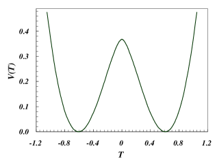
FIG. 1.: The shape of the symmetric potential in Eq. (7). The height is given by $V_{0}=e^{-1}$, while the minimum occurs for $T_{0}=1/\sqrt{e}$.

III Tachyon dynamics

Let us now address the problem of tachyon dynamics as governed by the action in Eq. (6). Let us begin by remarking that the expression we are using to model the profile of the potential has an unstable point. This is a false vacuum where the tachyon sits before condensation. Hereafter, we strictly assume that the tachyon is only the zero mode, it has no explicit dependence on any spatial dimensions. When tachyon condensates it sits at the minimum of the potential. In this process, the tachyon rolls down the potential and gradually forms a kink which becomes a stable $D3$ brane with a tension given by

$$T_{3}=V_{0}+T_{4}\,,$$ (8)

where $T_{3,4}$ are the brane tensions of $D3,\tilde{D4}$ branes. Notice, the tachyon being a homogeneous scalar field in our case can give rise a negative pressure. If the field is homogeneous within a patch of a Hubble size, then the patch may inflate the $3$ spatial dimensions. It turns out that a single tachyon system may not fulfill the required conditions, since it rolls down rather fast. However, if there is a set of unstable, parallel $\tilde{D4}$ branes separated from each other such that their tachyons do not interact among themselves, then inflation may occur. In order to simplify our situation we make some additional assumptions. One of the assumptions we have already mentioned and repeat here because of its importance. We treat the tachyon as a zero mode with a time dependence. This is related to the fact that presence of branes do not modify the underlying background space time structure. This allows us to write down the background world volume metric as

$$ds_{p+1}^{2}=dt^{2}-a^{2}(t)(dx_{1}^{2}+dx_{2}^{2}+dx_{3}^{2})-b^{2}\sum_{i=4}^{p}dx_{i}^{2}\,,$$ (9)

where $a(t)$ is the scale factor along the three spatial dimensions. The factor $b$ is not time dependent and it defines the common size of the extra spatial dimensions which we have assumed to be compactified on a torus. The actual value of $b$ is not crucial for our later discussion, although we take it to be of order of the fundamental string scale $(M_{\rm s})^{-1}$. Notice, that the metric is homogeneous and this apriori need not be the most general setup. However, we assume this for our purpose. The above metric only tells us that the branes are sitting on a space-time where there is no backreaction on the metric due to their presence. These simple assumptions allow us to understand the situation from $3+1$ dimensions.

Let us briefly comment on the mechanism which keeps the additional dimensions stable. There are couple of points to be noticed, first of all the common size of the additional dimensions is small. Therefore, it is easy to dynamically stabilize them. The fact that the radii are same leads to a single common radion mode from an effective $3+1$ dimensional point of view. The common mode has no dependence on the transverse spatial dimensions. The prescription of stabilizing the extra dimensions can be obtained dynamically following Ref. [13]. Here we simply recall some of its features. From the point of view of $3+1$ dimensions it is possible to provide a time varying positive running mass to the common mode. If the three spatial dimensions are expanding with a Hubble parameter $H$, then it has been observed in Ref. [13] that the common mode actually gets a running mass of order $\sim{\cal O}(H)$. Once this happens, the common mode decouples from the rest of the tachyon dynamics, and settles down to the minimum of its potential. This stabilizes the extra compact dimensions during the very first few e-foldings of inflation, thus, here onwards we can safely neglect their dynamics.

Let us now analyze in more details the dynamics of the tachyon as given by the potential in Eq. (7). This discussion is general and can be made in any arbitrary dimensions. The only difference is a scaling factor that enters on the potential, which shall appear due to integrating out the additional spatial dimensions. Since, $M_{\rm s}$ is close to the Planck scale, this scaling introduces only small factors which shall not affect the actual evolution of the tachyons. However, such a factor can play an important role while discussing density perturbations. For a moment we keep the discussion in units where $M_{\rm s}=1$.

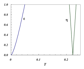
FIG. 2.: The two slow-roll parameters; $\epsilon$, and $\eta$, plotted with respect to the tachyon field $T$. Notice that the slow-roll conditions in Eq. (10) are not simultaneously satisfied as the field rolls down from top of the potential to the global minimum.

As it has been observed in Ref. [15] the tachyonic potential is expected to have a profile similar to that of a Mexican hat potential; $(T^{2}-T_{0}^{2})^{2}$ which is indeed the case of the potential in Eq. (7), see Fig. 1. Whether inflation takes place or not can be verified very easily, because most of the inflationary models are based on slow-roll inflation, which lays some simple conditions to be satisfied. In order to answer this query we study the inflationary conditions lead by the slow-roll parameters, which are given by

$$\epsilon\equiv\frac{1}{2}\left(\frac{V^{\prime}}{V}\right)^{2}\ll 1\,,\quad\quad\quad\eta\equiv\left|\frac{V^{\prime\prime}}{V}\right|\ll 1\,,$$ (10)

where prime denotes derivative with respect to the field. As expected the above conditions are not fulfilled at the same time during roll over of the field within a range $0\leq T\leq T_{0}\equiv 1/\sqrt{e}$. Indeed, one can easily check that at the top of the potential, $\epsilon$ is close to zero, because $V^{\prime}\approx 0$. However, $\eta$ is much larger than one. Since $V^{\prime\prime}(T)=4\ln T+6$, $\eta$ has a logarithmic divergence for $T\sim 0$, and remains large until the effective mass term for the potential vanishes at $T=e^{-3/2}$. On the other hand, as $\epsilon$ increases gradually, both parameters together never become less than one simultaneously, and thus the potential in Eq. (7) never provides a slow-roll inflation. This has been depicted in Fig. 2, where we have plotted $\epsilon$ and $\eta$. The field value where $V^{\prime\prime}$ vanishes is known as a spinodal point because at that point the mass squared term in the potential flips its sign from negative to positive. The conclusion is that the tachyon rolls down very fast and this was precisely the observation made already in Ref. [15].

For our potential inflation indeed takes place but for large values of $|T|>1$  [24], but this does not serve the present case. This rules out any possibility of having inflation with a single tachyon field. Alternative ideas have been discussed to cure this. Usually, it is believed that inflation might take place via altering the inter brane separation [15, 16]. In this paper we suggest a completely new way to address this problem. We suggest that inflation can be produced by a set of tachyonic fields, all with the same potential as given by Eq. (7). Such a scenario can appear from a system involving many non-interacting, and non-coincident parallel $\tilde{D4}$ branes in type IIB string theory. One of the key ingredients which we shall use here is the non-interacting property of the tachyons. Eventhough, these tachyons are not coupled to each other, they are coupled dynamically via the expansion of the Universe. This is an essence of assisted inflation which was originally discussed in Ref. [19]. Thus, the question we are interested in is asking whether we can have assisted inflation with a multi-tachyon configuration. This is the issue we shall study in coming sections.

IV Assisted inflation

A Toy model

In order to motivate the idea, we start by briefly recalling the main features of assisted inflation as originally presented in Ref. [19]. Let us begin with a set of exponential potentials of the form

$$V_{i}(\phi_{i})=V_{0}\exp\left(\alpha_{i}\,\phi_{i}\right)\,,$$ (11)

where each scalar field has an exponential potential with a different slope $\alpha_{i}$. Notice that the fields are not directly coupled, albeit the combined role of the fields affect the expansion rate of the Universe:

$$H^{2} = \frac{8\pi}{3m_{{\rm p}}^{2}}\sum_{i=1}^{n}\left[V_{i}(\phi_{i})+\frac{1}{2}\dot{\phi}_{i}^{2}\right]\,,$$ (12)

$$\ddot{\phi}_{i} = -3H\dot{\phi}_{i}-\frac{dV_{i}(\phi_{i})}{d\phi_{i}}\,,$$ (13)

where $H=\dot{a}/a$ is Hubble’s constant, $m_{\rm p}$ is the Planck scale, and $a$ is the scale factor of the flat FRW Universe in $3+1$ dimensions. Had there been a single field with an exponential potential, the solution would have been a power-law solution

$$a(t)\propto t^{p}\,,\quad\quad\quad p=\frac{16\pi}{m_{\rm p}^{2}\alpha^{2}}\,,$$ (14)

where $\alpha$ is assumed to be an arbitrary slope. Notice, that the solution is inflationary only if $p>1$, i.e. for extremely shallow exponentials; $\alpha\ll 1$. This suggests that if the potential is very steep, the field would roll down fast and there would be no inflation at all. Now let us imagine that all the fields have such a steep slopes and all of them are contributing to the dynamics, then the modified $\tilde{p}$ is given by

$$\tilde{p}=\frac{16\pi}{m_{{\rm p}}^{2}}\sum_{i=1}^{n}\frac{1}{\alpha_{i}^{2}}\,.$$ (15)

If we assume that all the slopes are the same then $\tilde{p}=np$. This suggests that potentials with $p<1$, which for a single field are unable to support inflation, can do so as long as there are enough scalar fields to make $np>1$. This means that more the scalar fields, the quicker is the expansion of the Universe. This is the reason the authors in Ref. [19] have named such a cumulative phenomena as assisted inflation. A generalization of this has been studied in a subsequent paper in Refs. [20], where various other potentials have been considered. There is a clear message from both the papers which we need to bear in mind that the dynamics of the assisted inflation works well only when the fields do not have any explicit couplings between themselves. Any kind of coupling tends to kill the assisted nature and this is the sole criterion which we also have to fulfill. There is another important reason behind choosing exponential potentials, because there exists a late time attractor solution for all the participating fields, see Refs. [19, 25]. This property is important while calculating the density perturbations generated by the scalar fields exactly. Lack of this behavior leaves the existing density perturbation calculations under some doubt.

B Our case

Our case is not very different from the analysis of the above toy model, but for the nature of the potential. As we have already discussed in section II if we consider a configuration of $n$ parallel non-BPS D4 branes which are separated from each other by a distance more than the string length, then there is a tachyon in the world volume theory of each brane and they donot interact with each other. The total potential from the tachyons for this configuration is just the sum of the potential from each tachyon and is given by

$$V=\sum_{i=1}^{n}V_{i}=\sum_{i=1}^{n}\left(T_{i}^{2}\ln T_{i}^{2}+V_{0}\right)\,,$$ (16)

where $n$ is the total number of tachyonic fields, or, in other words the total number of unstable non-BPS $D4$ branes, or, as a final configuration; the number of stable $D3$ branes. Notice, that the individual tachyons are as such unaware of each others presence except that they all support the Hubble expansion. Thus they are all in a dynamical contact. The inflationary scale has been implicitly assumed to be the string scale $\sim M_{\rm s}$. Due to our choice in the compactification the string scale can be related to the Planck scale by the compactification volume as $M_{s}^{2+n}\cdot vol\approx m_{\rm p}^{2}$.

The foremost point to notice is the following; for the potential Eq. (16), the slow-roll conditions are now different. They are given by

$$\epsilon_{i}\equiv\frac{1}{2}\left(\frac{1}{V}{\partial V\over\partial T_{i}}\right)^{2}\ll 1\,,\quad\quad\quad\eta_{i}\equiv\left|\frac{1}{V}{\partial^{2}V\over\partial T_{i}^{2}}\right|\ll 1\,,$$ (17)

As now the potential is a summation of all the tachyons present in spectrum, this changes the behavior of the slow-roll parameters. Our task is to ensure that they are both satisfied together while all $T_{i}$ roll down their respective potential. This can be seen very easily; let us assume for the time being that $T_{1}(t)\sim T_{2}(t)\sim,...,\sim T_{i}(t)\sim T(t)$, this means that all the trajectories are moving on a single line on a phase space diagram. This we will show later on. If we assume so, then the total potential becomes $V=nV_{1}$, and the slow-roll conditions become

$$\epsilon_{i}\sim\left(\frac{1}{n^{2}}\right)\epsilon\,,\quad\quad\quad\eta_{i}\sim\left(\frac{1}{n}\right)\eta\,,$$ (18)

where $\epsilon$ and $\eta$ are given as for a single field case,

$$\epsilon={1\over 2}\left[{2T\left(\ln T^{2}+1\right)\over T^{2}\ln T^{2}+V_{0}}\right]^{2}~{};\qquad\eta={|\ln T^{4}+6|\over T^{2}\ln T^{2}+V_{0}}~{}.$$ (19)

Next, our objective is to obtain the minimal number of branes required to obtain a region in the field space where $\eta_{i}$ and $\epsilon_{i}$ can be made smaller than one in order to satisfy the slow-roll conditions. Notice, that around $T=0$, $\eta_{i}$ still has a logarithmic divergence. Therefore, we do not expect that the slow-roll conditions be satisfied right on top of the tachyon potential. However, as the fields roll down their respective potential, there exists a domain where $\epsilon_{i}$ can be made less than one along with $\eta_{i}$. The valid region holds good until $T=e^{-3/2}$, the point where $\eta$ goes to zero. Therefore, if we demand that $\epsilon_{i}(e^{-3/2})\ll 1$, we can estimate the number of branes needed to suppress $\epsilon$, and, $\eta$. This gives

$$n\gg\sqrt{\epsilon(e^{-3/2})}={\sqrt{8}\over\sqrt{e}\left(1-3e^{-2}\right)}\approx 2.89~{}.$$ (20)

For instance, if one requires $\epsilon_{i}<0.1$ around the spinodal point $T=e^{-3/2}$, we will need a larger number of non-interacting $\tilde{D4}$ branes. In fact the number of branes turns out to be $n\geq 10$.

One can check the above statements by plotting $\epsilon_{i}$, and $\eta_{i}$ with respect to an arbitrary $T_{i}$, and looking for the region in field space where both the slow-roll parameters are less than one. In order to illustrate this point we have plotted in Fig. 3 the slow-roll parameters as given by Eq. (18), for $n=10$. The large number of fields add up in the potential which ultimately affects the Hubble expansion of the Universe. As a result the slow-roll conditions Eq. (10) are satisfied simultaneously for field values ranging from $0.1<T_{i}<0.3$. As we increase the number of fields, the overlapping region widens up. This is the desired feature of assisted inflation which we wanted in our case. Assisted inflation by multi-tachyon really helps to inflate our three spatial dimensions, which are the longitudinal direction of all the $D3$ branes system. This is a unique feature which shows an intrinsic characteristic of all the branes. We do not require an uncertainty of moving the branes in a higher dimensional space time. Even if the branes have a slow relative motion, our scenario can be realizable. All it requires is that the tachyons developing an individual kink does not communicate with others. We should mention that last condition can be easily realized as long as the inter brane separation is larger than the string scale and the branes remain parallel to each other. In this paper we do not intend to find out an exact form of the scale factor, which we do not actually require for the density perturbation calculation. Finally, let us note here the versatile nature of the occurrence of the potential Eq. (7). The potential can occur in one-loop supersymmetric corrections to the masses in a bosonic sector, which gives a running mass to the field. This is a common feature while studying inflation in supersymmetric theories.

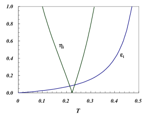
FIG. 3.: The two slow-roll parameters; $\epsilon_{i}$, and $\eta_{i}$ are plotted with respect to a single tachyon field $T_{i}$ when the total number of tachyons is taken to be $n=10$. Notice, now the slow-roll conditions can be satisfied concurrently in the region where the tachyonic fields are rolling down their respective potentials.

Inflation apart from making the Universe very flat also generates density perturbation causally. What actually matters is the last number of e-foldings before the end of inflation. This is because the observable Universe has to be well within the horizon at the time of density perturbations are being produced. The number of e-foldings thus required is a model dependent issue, which involves the uncertainty of two important scales; one at which inflation takes place, and the other, the temperature at which the Universe becomes radiation dominated. In our case we fix the inflationary scale to be the string scale and in the next section we delve into the reheating temperature of the Universe.

Before we move onto that we briefly mention the dynamics of the tachyon fields. Notice, that the equations of motion for the tachyons in $3+1$ dimension follow a simple relationship:

$$\frac{\dot{T}_{i}}{\dot{T}_{1}}=\frac{T_{i}}{T_{1}}\frac{1+2\ln T_{i}}{1+2\ln T_{1}}\,,\quad\quad\quad{\rm for~{}~{}~{}i\neq 1}\,,$$ (21)

where dot denotes derivative with respect to time. While deriving the above equation we have assumed the slow-roll conditions to be valid for all the tachyons. We notice, that in the interesting regime $|\ln T_{i}|\gg 1/2$, the above expressions can be easily rewritten in a form

$${d\over dt}(\ln\left(\ln T_{i}\right))={d\over dt}(\ln\left(\ln T_{1}\right))~{}.$$ (22)

The above relationship is very important. It ensures that if the slow-roll conditions are satisfied, then there can be an unique solution, which tells us that all the tachyons follow a similar trajectory with an unique late time attractor, such that

$$T_{1}(t)\sim T_{2}(t)\sim\,,...\,,\sim T_{i}(t)\,.$$ (23)

This is an interesting result, because other than the exponential potentials, such a late time attractor behavior is very rare. In our case, it holds for a wide region of phase space, all that it requires is that during the slow-roll inflation all the tachyons must follow $|\ln T_{i}|\gg 1/2$, which is very genuine. This allows us to perform the density perturbation calculation without any doubt.

V Density perturbations and reheating

In this section we estimate the amplitude of the density perturbations produced during inflation, and, the reheating temperature of the Universe. While generating the density perturbations the tachyon trajectories follow Eq. (23). We pursue our calculation of density perturbation following Refs. [26, 19], which depends crucially on the late time attractor behavior of the fields. The Hubble expansion in our case is a cumulative effect of all the stable BPS $D3$ branes which can be expressed as

$$H^{2}\approx\frac{8\pi}{3m_{\rm p}^{2}}n{V_{eff}}~{},$$ (24)

where we considered the potential contribution alone by assuming the slow-roll conditions Eq. (10) are met. Here, we have also assumed there are $n$ tachyons with the same effective $3+1$ dimensional potential $V_{eff}$, which has to be calculated after integrating out the transverse dimensions in Eq. (6). The effect is a scaling on the potential such that $V_{eff}=vol\cdot V$. By assuming that the transverse directions are compactified on a torii, we can obtain the effective potential in $3+1$ dimensions as

$$V_{eff}(T)=M_{s}^{2}\left[T^{2}\ln\left({T\over m_{\rm p}}\right)^{2}+m_{\rm p}^{2}V_{0}\right]\,.$$ (25)

The amplitude of the perturbations can be calculated before the end of inflation while the tachyons are rolling down towards their respective minima. Since, tachyons follow the trajectory given by Eq. (23), we can directly follow the results obtained in Refs. [19, 26]. We obtain the spectrum of the density perturbations is given by

$$\delta_{H}(k)\approx{1\over 5\pi}{H^{2}\over\sqrt{n}~{}|\dot{T}|}={3n\over 5\pi}~{}{V_{eff}^{3/2}\over m_{\rm p}|V^{\prime}_{eff}|}~{},$$ (26)

where one has to evaluate the right hand side at the moment when the perturbations are leaving the horizon, which one can roughly considered to be the critical point $T\sim e^{-3/2}m_{\rm p}$. This assumption restricts the tachyon trajectories before the last $50-60$ e-foldings of inflation as we have mentioned above. This is what counts for the observable Universe. Our estimation then gives

$$\delta_{H}(k)\approx\left({3nM_{s}\over 20\pi m_{\rm p}}\right)\left(1-3e^{-2}\right)^{3/2}\sim 2\cdot 10^{-2}\left(nM_{s}\over m_{\rm p}\right).$$ (27)

The overall amplitude of the density perturbations is constrained by COBE, which predicts the right hand side of Eq. (27) to be $\sim 10^{-5}$. Therefore, in order to be consistent with a COBE result, we need to constrain either the fundamental scale $M_{\rm s}$, or, the number of tachyons required. The lower the ratio $M_{\rm s}/m_{\rm p}$ is, the higher the required number of non-coincident unstable branes. If we suppose $n\geq 10$ as needed for inflation, then the string scale is constrained; we get $M_{\rm s}\sim 10^{(-2,-3)}m_{\rm p}/n\leq 10^{(-3,-4)}m_{\rm p}$. Our naive estimation suggests that if the string scale is around the Grand Unification scale, then the required number of unstable branes can be about ten.

All the tachyons while inflating the Universe reach a particular point on the field space where the slow-roll conditions break down. This obviously depends on the number of tachyons we have in the spectrum, see Eq. (17). Once, inflation ends, the era of entropy production prevails. This is the first natural step among the post-inflationary epochs. The Universe is required to be heated up to provide a thermal bath with a radiation dominated Universe. In the conventional inflationary models it is believed that the classical energy stored in the inflaton potential is converted into the kinetic energy of the radiation bath through which one can easily estimate the final reheat temperature. The situation in our case is similar to the traditional one. The final scenario of reheating may go as follows. After the tachyons have rolled down the potential, they begin oscillations around the minimum. Notice, the following; the tachyon forms a kink in order to form a stable $D3$ brane. After forming the kink the tachyon has to completely decay. Part of its energy density in a region where the $D3$ brane has formed goes into the brane tension. However, rest of the vacuum energy, that originally out of the kink has to be released in a way that produces a thermal bath in the bulk. This happens while tachyons oscillate around their minimum. The oscillations lead to a time variation in the width of the kink. This in turn leads to a vacuum instability. This phenomena has a similar feature as a parametric reheating of the Universe, where the coherent oscillations of the classical vacuum produces quanta in a non-thermal way. In our case, the massless zero mode gauge fields are excited, possibly along with the massive gauge fields appearing due to compactification of the spatial dimension.

The main conclusion is that the total energy stored in the region where the tachyon has gone to the minimum can be released into exciting the gauge fields, while the energy in the region where the kink has formed shall be translated into the brane tension following Sen’s conjecture. The final reheat temperature can be estimated if we assume that the tachyons only couple to the gauge fields with some gauge coupling $\sim\alpha_{s}$, same for all tachyons, then an approximate reheat temperature can be estimated by [1]

$$T_{rh}\approx 0.1\sqrt{\alpha_{s}^{2}M_{\rm s}m_{\rm p}}\,.$$ (28)

While writing the above expression we have however assumed that the tachyon mass is determined by its vacuum configuration which is given by the string scale $\sim M_{\rm s}$. This might leads to a very high reheat temperature $T_{rh}\leq\alpha_{s}\cdot 10^{16}$ GeV. Such a high reheat temperature might not be acceptable on many other cosmological grounds, which warrants another phase of late inflation in order to dilute any unwanted species. A late decay of those heavy modes produced by the tachyon may also help to modify the above relationship bringing $T_{rh}$ much smaller.

VI Conclusion

Let us summarize our results. Starting from the observation that a non-BPS $D4$ brane can decay into a stable $D3$ brane via tachyon condensation, we imagine this process as a dynamical one which might give rise to some interesting cosmological phenomena. Then we have studied a single tachyon case to show that inflation is not possible while the tachyon is rolling down the potential because the usual potential supported from the string field theory comes out to be too steep. The two slow-roll conditions are not simultaneously satisfied and the tachyon rolls rather fast. However, as we have argued, if there is a set of parallel and non-coincident unstable non-BPS branes, then tachyon condensation may lead to a successful inflation where both the slow-roll conditions can be met simultaneously. This is a virtue of a multi field dynamics where the tachyons do not interact among themselves but tied up with the evolution of the Universe. In this setup the Universe can be imagined to be a set of parallel $D3$ branes. For the specific tachyonic potential which we have considered here, we noticed that one requires at least more than three non-BPS $D4$ branes to fulfill all our criterion and drive inflation. A more conservative point of view requires at least ten such branes. We have noticed that while the tachyons are rolling down the potential they can generate density perturbations which can match the observed COBE normalization. The final fate of the tachyons in each and every brane is to form a kink, identified as the final BPS $D3$ brane whose tension is given by the tachyon energy trapped with the kink. The left over vacuum where the kink does not form releases its energy while the tachyon is oscillating around the true minimum, thus reheating the world. Our estimation towards the reheat temperature is quite large. This is because the gauge fields which are coupled to the tachyons have a string coupling. The tachyon condensates at a value close to the string scale giving rise to massive gauge fields. The massive gauge fields also decay and they are all responsible for generating further entropy, that may help to reduce our current estimation of the reheating temperature.

- [1] A. Guth, Phys. Rev. D 23, 347 (1981); A. D. Linde, Particle Physics and Inflationary Cosmology, Harwood Chur (1990); E. W. Kolb and M. S. Turner, The Early Universe, Addison–Wesley, Redwood City (1990); A. R. Liddle and D. H. Lyth, Cosmological Inflation and Large-Scale Structure, Cambridge University Press (2000).
- [2] E. F. Bunn, D. Scott and M. White, Ap. J. 441, L9 (1995); E. F. Bunn and M. White, Ap. J 480, 6 (1997).
- [3] P. Binetruy and M. K. Gaillard, Phys. Rev. D 34, 3069 (1986).
- [4] T. Banks, hep-ph/9906126; hep-th/9911067
- [5] R. Brustein and P.J. Steinhardt, Phys. Lett. B 302, 196 (1993); T. Banks, D. Kaplan and A. Nelson, Phys. Rev. D 49, 779 (1994); B. de Carlos, J.A. Casas, F. Quevedo and E. Roulet, Phys. Lett. B 318, 447 (1993).
- [6] J. Polchinski, String Theory, Cambridge University Press (1998).
- [7] A. Sen, JHEP9912, 027 (1999).
- [8] O. Bergman and M. R. Gaberdiel, Phys. Lett. B 441, 133 (1998).
- [9] A. Sen, hep-th/9904207.
- [10] I. Antoniadis, Phys. Lett. B246, 377 (1990); I. Antoniadis, K. Benakli and M. Quirós, Phys. Lett. B331, 313 (1994); K. Benakli, Phys. Rev. D60, 104002 (1999); Phys. Lett. B 447, 51 (1999); N.Arkani-Hamed, S. Dimopoulos, and G. Dvali, Phys. Lett B 429, 263 (1998); Phys. Rev. D 59, 086004 (1999); I. Antoniadis, N. Arkani-Hamed, S. Dimopoulos, and G. Dvali, Phys. Lett. B 436, 257 (1998); L. Randall and R. Sundrum, Phys. Rev. Lett. 83, 4690 (1999); L. Randall and R. Sundrum, Phys. Rev. Lett. 83, 3370 (1999).
- [11] D. H. Lyth, Phys. Lett. B 448, 191 (1999); G. Dvali and S. H. H. Tye, Phys. lett. B 450, 72 (1999); N. Kaloper and A. Linde, Phys. Rev. D 59, 10130 (1999); A. Mazumdar, Phys. Lett. B 469, 55 (1999); N. Arkani-Hamed, S. Dimopoulos, N. kaloper and J. March-Russell, Nucl. Phys. B 567, 189 (2000); R. N. Mohapatra, A. Pérez-Lorenzana and C. A. de S. Pires, Phys. Rev. D 62, 105030 (1999).
- [12] A. Lukas, B. A. Ovrut and D. Waldram, Phys. Rev. D 61, 023506 (2000); P. Binetruy, C. Deffayet and D. Langlois, Nucl. Phys. B 565, 269 (2000); P. Binetruy, C. Deffayet, U. Ellwanger and D. Langlois, Phys. Lett. B 477, 285 (2000); R.N. Mohapatra, A. Pérez-Lorenzana and C.A. de S. Pires, Int. J. Mod. Phys. A 16, 1431 (2001). A. Lukas and D. Skinner, hep-th/0106190.
- [13] A. Mazumdar and A. Pérez-Lorenzana, Phys. Lett. B 508, 340 (2001).
- [14] S. Alexander, hep-th/010503.
- [15] C. P. Burgess, M. Majumdar, D. Nolte, F. Quevedo, G. Rajesh and R.-J. Zhang, hep-th/0105204.
- [16] G. Dvali, Q. Shafi and S. Solganik, hep-th/0105203; G. Shiu and S.-H. Tye, hep-th/0106274.
- [17] J. Khoury, B. A. Ovrut, P. J. Steinhardt and N. Turok, hep-th/0103229; hep-th/0105199; hep-th/0105212; K. Enqvist, E. Keski-Vakkuri and S. Rasanen, hep-th/0106282.
- [18] R. Kallosh, L. Kofman and A. Linde, hep-th/0104073; hep-th/0106241.
- [19] A. R. Liddle, A. Mazumdar and F. E. Schunck, Phys. Rev. D 58, 061301 (1998).
- [20] E.J. Copeland, A. Mazumdar and N.J. Nunes, Phys. Rev.D 60, 083506 (1999); A. M. Green and J. E. Lidsey, Phys. Rev. D 61, 067301 (2000).
- [21] A. Sen, JHEP 9910, 008 (1999).
- [22] E.A. Bergshoeff, M. de Roo, T.C. de Wit, E. Eyras and S. Panda, JHEP 0005, 009 (2000).
- [23] J. A. Minhan and B. Zwiebach, JHEP 0009, 029 (2000); JHEP 0010, 045 (2000).
- [24] J. D. Barrow and P. Parsons, Phys. Rev. D 52, 5576 (1995).
- [25] K. A. Malik and D. Wands, Phys. Rev. D 59, 123501 (1999).
- [26] M. Sasaki and E. D. Stewart, Prog. Theor. Phys. 95, 71 (1996).