Study of ${B}^{0}\to J/\Psi D^{(\star)}$ and $\eta_{c}D^{(\star)}$ in Perturbative QCD

Abstract

Motivated by recent interest in soft $J/\Psi$ production in $B$ decays, we investigate ${B}^{0}\to J/\Psi D^{(\star)}$ and $\eta_{c}D^{(\star)}$ decays in perturbative QCD. We find that, within that framework, these decays are calculable since the heavy $c\bar{c}$ pair in the final states is created by a hard gluon. The branching ratios are estimated to be around $10^{-7}\sim 10^{-8}$, too small to be consistent with the data, suggesting that other mechanism(s) contribute to the observed excess of soft $J/\Psi$ in ${B}^{0}\to J/\Psi+X$ decays. The possibility of the production of a hybrid $s{\bar{d}}g$ meson with mass about $2$ GeV is briefly entertained.

PACS Numbers: 12.38Bx, 12.39Jh

Keywords: $B$-meson, charmonium, $D$ meson, $D^{\star}$ meson, hybrid meson

With the advent of the BaBar and Belle $B$ factories, many $B$ decay modes could be studied in detail. The rich phenomena of $B$ decays will provide testing grounds for theories of weak interactions and hadrons. It is interesting to note that measurements of the inclusive $B\to J/\Psi X$ spectrum by CLEO [1] and recently by Belle [2], indicate a hump for low $J/\Psi$ momentum, which kinematically corresponds to $J/\Psi$ recoiling against a partner as heavy as $\sim 2~{}{\rm GeV}$. Brodsky and Navarra [4] suggest that the $J/\Psi$ hump may be due to the decay ${B}^{0}\to J/\Psi\Lambda\bar{p}$ with possible formation of $\Lambda-\bar{p}$ bound state (an exotic strange baryonium).

From another view point, Chang and Hou [3] proposed as an explanation the existence of intrinsic charm in the $B$ meson which decays as ${B}^{0}(\bar{d}bc\bar{c})\to J/\Psi D^{(*)}$ (and similarly for $\eta_{c}$ instead of $J/\Psi$). Thus the intrinsic charm pair transforms into a $c{\bar{c}}$ final state while the $b$ decays. It is argued that a rate of $\sim 10^{-4}$ may be possible in this way if the intrinsic charm content of $B$ is not much less than $1\%$.

We raise here another possibility: The $B$ may decay into a charmonium plus a hybrid, $B^{0}\to J/\Psi H$, where $H$ is a hybrid $s{\bar{d}}g$ [5] with $M_{H}\approx 2~{}{\rm GeV}$ [6]. Two diagrams that contribute to such a process are depicted in Fig. 1. Note that the gluons exchanged in Fig. 1 are soft while those in Fig. 2 (i.e. for the conventional $B^{0}\to J/\Psi D^{(*)}$, see below) are hard, thus enhancing the hybrid option as compared to the conventional approach for $B^{0}\to J/\Psi D^{(*)}$. In addition, as shown below, each Feynman diagram in Fig. 2 involves one fermion and one hard gluon propagator with average virtuality as large as $10~{}{\rm GeV}^{2}$. So, we can expect the $B^{0}\to J/\Psi H$ decay rate to be $10^{3}\sim 10^{4}$ times larger than $B^{0}\to J/\Psi D^{(*)}$, although a reliable quantitative estimate of the decay rate is very difficult.

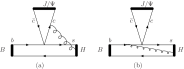
Figure 1: Examples of Feynman diagrams for the production of a hybrid $H=s{\bar{d}}g$ in ${B}^{0}\to J/\Psi H$.

To make such “exotic” suggestions more reliable, one should be convinced that the conventional picture of heavy mesons indeed leads to tiny numbers in disagreement with experiment. To our knowledge, such study is still not available in the literature. In this article we investigate these decays within the conventional picture of heavy mesons having the minimal number of quarks and using perturbative QCD (pQCD). The applicability of pQCD is justified by the large virtuality of the hard gluon which creates a $c\bar{c}$ pair. As known, in many applications of pQCD to B decays [8], say $B\to\pi\pi$, the virtuality of the gluon in the hard kernel scales like $k^{2}_{g}\simeq-M_{B}\Lambda_{\rm{QCD}}x\simeq-2x~{}\rm{GeV}^{2}$, where $x$ is the momentum fraction carried by the light spectator quark in the final light meson. However in the processes discussed in this paper (see Fig. 2), the gluon virtuality scales as $k^{2}_{g}>(2m_{c})^{2}$. Furthermore, under the common assumption of factorization, there are no infrared divergences which cannot be absorbed in wave function, or large end point contributions.

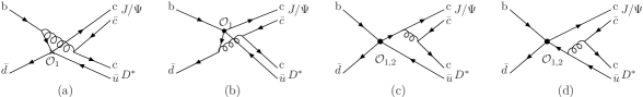
Figure 2: Feynman diagrams for ${B}^{0}\to J/\Psi D^{(*)}$ in pQCD.

We begin our calculation of the decays ${B}^{0}\to J/\Psi D^{(*)}$ within the pQCD approach for exclusive QCD processes [7] as depicted in Fig. 2, by writing the weak effective Hamiltonian $H_{\rm eff}$ for the $b\to c\bar{u}d$ transitions as [9]

$${\cal H}_{\rm eff}=\frac{G_{F}}{\sqrt{2}}V_{cb}V_{ud}^{*}\left[C_{1}(\mu)\bar{d}\gamma_{\mu}(1-\gamma_{5})u\,\bar{c}\gamma^{\mu}(1-\gamma_{5})b+C_{2}(\mu)\bar{c}\gamma_{\mu}(1-\gamma_{5})u\,\bar{d}\gamma^{\mu}(1-\gamma_{5})b\right],$$ (1)

where the Wilson coefficients $C_{1,2}(\mu)$ are evaluated to be $C_{1}(m_{b})=1.124$ and $C_{2}(m_{b})=-0.273$ at the scale $\mu=m_{b}=4.8~{}{\rm GeV}$ [10].

To calculate the amplitudes of the Feynman diagrams in Fig. 2, we take the wave functions for ${B}^{0}$, $J/\Psi$ and $D^{*}$ as follows [11, 8]

$${\bf\Psi}_{B} = \frac{i}{4N_{c}}(\not P_{B}+M_{B})\gamma_{5}\phi_{B}(x)f_{B},$$ (2)

$${\bf\Psi}_{V} = -\frac{1}{4N_{c}}\not\varepsilon(M_{V}+\not P_{V})\phi_{V}(x)f_{V},~{}~{}~{}(V=J/\Psi,D^{*}).$$ (3)

Now we can write the amplitudes of Fig. 2. as

$${\cal M}_{a} = -if_{B}f_{\Psi}f_{D^{*}}\pi\alpha_{s}\frac{1}{16}\frac{C_{F}}{N^{2}_{c}}C_{1}\int dxdydz\phi_{B}(x)\phi_{\Psi}(y)\phi_{D^{*}}(z)\frac{1}{D_{a}}\frac{1}{k^{2}}$$ (4)

$$\times{\rm Tr}[(\not{P}_{B}+M_{B})\gamma_{5}\gamma_{\mu}(1-\gamma_{5})((1-x)\not{P}_{B}-\not{k}+m_{b})\gamma_{\nu}]$$

$$\times{\rm Tr}[\not{\varepsilon}_{\Psi}(M_{\Psi}+\not{P}_{\Psi})\gamma^{\mu}(1-\gamma_{5})\not{\varepsilon}_{D^{*}}(M_{D^{*}}+\not{P}_{D^{*}})\gamma^{\nu}],$$

$${\cal M}_{b} = -if_{B}f_{\Psi}f_{D^{*}}\pi\alpha_{s}\frac{1}{16}\frac{C_{F}}{N^{2}_{c}}C_{1}\int dxdydz\phi_{B}(x)\phi_{\Psi}(y)\phi_{D^{*}}(z)\frac{1}{D_{b}}\frac{1}{k^{2}}$$ (5)

$$\times{\rm Tr}[(\not{P}_{B}+M_{B})\gamma_{5}\gamma_{\nu}(\not{k}-x\not{P}_{B})\gamma_{\mu}(1-\gamma_{5})]$$

$$\times{\rm Tr}[\not{\varepsilon}_{\Psi}(M_{\Psi}+\not{P}_{\Psi})\gamma^{\mu}(1-\gamma_{5})\not{\varepsilon}_{D^{*}}(M_{D^{*}}+\not{P}_{D^{*}})\gamma^{\nu}],$$

$${\cal M}_{c} = -if_{B}f_{\Psi}f_{D^{*}}\pi\alpha_{s}\frac{1}{16}\left(\frac{C_{F}}{N^{2}_{c}}C_{1}+\frac{C_{F}}{N_{c}}C_{2}\right)\int dxdydz\phi_{B}(x)\phi_{\Psi}(y)\phi_{D^{*}}(z)\frac{1}{D_{c}}\frac{1}{k^{2}}$$ (6)

$$\times{\rm Tr}[(\not{P}_{B}+M_{B})\gamma_{5}\gamma_{\mu}(1-\gamma_{5})]{\rm Tr}[\not{\varepsilon}_{\Psi}(M_{\Psi}+\not{P}_{\Psi})\gamma_{\nu}(\not{P}_{\Psi}+\not{k}+m_{c})$$

$$\gamma^{\mu}(1-\gamma_{5})\not{\varepsilon}_{D^{*}}(M_{D^{*}}+\not{P}_{D^{*}})\gamma^{\nu}],$$

$${\cal M}_{d} = if_{B}f_{\Psi}f_{D^{*}}\pi\alpha_{s}\frac{1}{16}\left(\frac{C_{F}}{N^{2}_{c}}C_{1}+\frac{C_{F}}{N_{c}}C_{2}\right)\int dxdydz\phi_{B}(x)\phi_{\Psi}(y)\phi_{D^{*}}(z)\frac{1}{D_{d}}\frac{1}{k^{2}}$$ (7)

$$\times{\rm Tr}[(\not{P}_{B}+M_{B})\gamma_{5}\gamma_{\mu}(1-\gamma_{5})]{\rm Tr}[\not{\varepsilon}_{\Psi}(M_{\Psi}+\not{P}_{\Psi})\gamma^{\mu}(1-\gamma_{5})$$

$$((1-z)\not{P}_{D^{*}}+\not{k})\ \gamma_{\nu}\not{\varepsilon}_{D^{*}}(M_{D^{*}}+\not{P}_{D^{*}})\gamma^{\nu}],$$

where $C_{F}=\frac{4}{3}$ and $N_{c}=3$ is the number of colors. $D_{i}(i=a,b,c,d)$ and $k^{2}$ denote the virtuality of quark and gluon propagators in Fig. 2.$i$, which are given by

$$D_{a} = -m^{2}_{b}+M^{2}_{B}(1-x-y)(1-x-z)+(y-z)(M^{2}_{\Psi}(x+y-1)-M^{2}_{D^{*}}(x+z-1))$$ (8)

$$-i\epsilon,$$

$$D_{b} = M^{2}_{B}(x-y)(x-z)+(y-z)(M^{2}_{\Psi}(y-x)+M^{2}_{D^{*}}(x-z))-i\epsilon,$$ (9)

$$D_{c} = -m^{2}_{c}+M^{2}_{\Psi}(1-z)+(M^{2}_{B}-M^{2}_{D^{*}}(1-z))z-i\epsilon,$$ (10)

$$D_{d} = \frac{1}{2}(M^{2}_{B}(1+2y-z)+M^{2}_{D^{*}}(1-2y+z)+M^{2}_{\Psi}(2y^{2}-2yz+z-1))-i\epsilon,$$ (11)

$$k^{2} = M^{2}_{\Psi}y(y-z)+z(M^{2}_{B}y+M^{2}_{D^{*}}(z-y))-i\epsilon.$$ (12)

It may be instructive to evaluate typical virtualities of the propagators involved in pQCD calculations. Taking $x=1-m_{b}/M_{B},\,y=1/2$ and $z=m_{c}/M_{D^{*}}$, we find

$$D_{a}=-20.4~{}{\rm GeV}^{2},\,\,D_{b}=7.2~{}{\rm GeV}^{2},\,\,D_{c}=20.2~{}{\rm GeV}^{2},\,\,D_{d}=16.4~{}{\rm GeV}^{2},\,\,k^{2}=9.9~{}{\rm GeV}^{2}.$$ (13)

These values are large enough to justify our pQCD calculation.

The amplitude for ${B}^{0}\to J/\Psi D^{*}$ is decomposed as

$$A({B}\to J/\Psi(P_{\Psi})D^{*}(P_{D^{*}}))=\varepsilon^{\mu}_{\Psi}\varepsilon^{\nu}_{D^{*}}({\cal S}~{}g_{\mu\nu}+{\cal D}~{}P_{D^{*}\mu}P_{\Psi\nu}+i{\cal P}~{}\epsilon_{\mu\nu\alpha\beta}P^{\mu}_{\Psi}P^{\nu}_{D*}),$$ (14)

where the coefficients ${\cal S}$, ${\cal P}$ and ${\cal D}$ correspond to $s$, $p$ and $d$ wave amplitudes, respectively, and can be evaluated from Eqs. 4 to 7. The helicity amplitudes are constructed to be

$$H_{00} = \frac{1}{2M_{\Psi}M_{D^{*}}}\left[{\cal S}(M^{2}_{B}-M^{2}_{\Psi}-M^{2}_{D^{*}})+2{\cal D}M^{2}_{B}|{\bf p}|^{2}\right],$$

$$H_{\pm\pm} = -({\cal S}\pm{\cal P}M_{B}|{\bf p}|).$$ (15)

The branching ratio is given by

$${\rm Br}({B}^{0}\to J/\Psi D^{*})=\tau_{{B}^{0}}\frac{|{\bf p}|}{8\pi M^{2}_{B}}\frac{G^{2}_{F}}{2}|V_{cb}|^{2}\left(|H_{00}|^{2}+|H_{++}|^{2}+|H_{--}|^{2}\right).$$ (16)

Since the $b$ and $c$ quarks are heavy and their mass is much larger than the typical QCD scale $\Lambda_{\rm QCD}$ for a bound state, we can expect that the distribution functions of heavy mesons will peak around the points where the heavy quarks are near their mass shell with variance $\Lambda_{\rm QCD}/m_{Q}$. As an ansatz, the distribution functions are taken as

$$\phi_{B}(x)=\delta(x-x_{B}),\,\,\phi_{\Psi}(y)=\delta(y-y_{\Psi}),\,\,\phi_{D^{*}}(z)=\delta(z-z_{D^{*}}),$$ (17)

with $x_{B}=1-\frac{m_{b}}{M_{B}}$, $y_{\Psi}=\frac{1}{2}$ and $z_{D^{*}}=\frac{m_{c}}{M_{D^{*}}}$.

To get numerical results, we use $V_{cb}=0.04,~{}f_{B}=180~{}{\rm MeV},~{}~{}f_{\Psi}=400~{}{\rm MeV},~{}~{}f_{D^{*}}=230~{}{\rm MeV},~{}~{}m_{b}=4.8~{}{\rm GeV},~{}M_{{B}^{0}}=5.27~{}{\rm GeV},~{}m_{c}=1.4~{}{\rm GeV},~{}M_{\Psi}=3.1~{}{\rm GeV},~{}M_{D^{*}}=2~{}{\rm GeV},~{}\alpha_{s}(2m_{c})=0.266$. We get

$${\rm Br}({B}^{0}\to J/\Psi D^{*})=6.46\times 10^{-8},$$ (18)

and the longitudinal polarization fraction is

$$P_{L}=\frac{\Gamma_{L}}{\Gamma}=0.398.$$ (19)

Since the amplitudes are highly suppressed by the large virtualities of the propagators as shown in Eqs. 8 to 13, the smallness of ${\rm Br}({B}^{0}\to J/\Psi D^{*})$ is understandable. To illustrate the stability of our results, we plot in Fig. 3 ${\rm Br}({B}^{0}\to J/\Psi D^{*})$ versus $x_{B}$, i.e., the peak point of $\phi_{B}(x)$.

Figure 3: ${\rm Br}({B}^{0}\to J/\Psi D^{*})$ vs. $x_{B}$, the peak point of $\phi_{B}(x)$.

From Fig. 3, we can see that the rate is rather stable against changes of the parameter $x_{B}$. Due to relativistic effects, the distribution functions should have variances of ${\cal O}(\Lambda_{\rm QCD}/m_{Q})$. To show the effects of the variances, we take

$$\phi_{B}(x) = N_{B}x(1-x)\exp\left[-\left(\frac{M_{B}}{M_{B}-m_{b}}\right)^{2}\left(x-x_{B}\right)^{2}\right],$$ (20)

$$\phi_{D^{*}}(x) = N_{D^{*}}x(1-x)\exp\left[-\left(\frac{M_{D^{*}}}{M_{D^{*}}-m_{c}}\right)^{2}\left(x-x_{D^{*}}\right)^{2}\right],$$ (21)

$$\phi_{\Psi}(x) = N_{\Psi}x(1-x)\exp\left[-\left(\frac{M_{\Psi}}{M_{\Psi}-2m_{c}}\right)^{2}\left(x-\frac{1}{2}\right)^{2}\right],$$ (22)

where $N_{B}$, $N_{D^{*}}$ and $N_{\Psi}$ are normalization constants to make $\int dx\phi(x)=1$. To model the distribution functions, we take the mass difference between the heavy meson and its heavy constituent(s) as shape parameter. These distribution functions follow the consensus that the smaller the mass difference the sharper the distribution functions. Using these distribution functions, we obtain

$${\rm Br}({B}^{0}\to J/\Psi D^{*})=8.50\times 10^{-8},~{}~{}~{}P_{L}=\frac{\Gamma_{L}}{\Gamma}=0.395.$$ (23)

Since ${B}^{0}$ decays with three charm quarks in its final states, it could be taken as a probe of strong interactions, especially hadron dynamics. We extend our calculations to ${B}^{0}\to J/\Psi D,\,\eta_{c}D$ and $\eta_{c}D^{*}$ decays. The amplitudes for these decays can be obtained through the following replacements in Eqs. 3 to 7

$${\bf\Psi}_{D^{*}}\longrightarrow{\bf\Psi}_{D} = \frac{i}{4N_{c}}\gamma_{5}(\not\!P_{D}\,+M_{D})\phi_{D}(x)f_{D},$$

$${\bf\Psi}_{\Psi}\longrightarrow{\bf\Psi}_{\eta_{c}} = \frac{i}{4N_{c}}\gamma_{5}(\not\!P_{\eta_{c}}\,+M_{\eta_{c}})\phi_{\eta_{c}}(x)f_{\eta_{c}}.$$ (24)

Using $f_{D}=200~{}{\rm MeV}$, $f_{\eta_{c}}=335~{}{\rm MeV}$, the branching ratios are estimated to be

$${\rm Br}({B}^{0}\to J/\Psi D) = 7.28\times 10^{-8},$$

$${\rm Br}({B}^{0}\to\eta_{c}D^{*}) = 1.39\times 10^{-7},$$

$${\rm Br}({B}^{0}\to\eta_{c}D) = 1.52\times 10^{-7}.$$ (25)

In summary, we have studied the decays ${B}^{0}\to J/\Psi(\eta_{c})D^{(*)}$ within the conventional theoretical framework. The branching ratios of these decays are estimated to be around $10^{-7}\sim 10^{-8}$. ${B}^{0}$ decays to $J/\Psi D^{(*)}$ can not account for the excess for slow $J/\Psi$ as indicated by the CLEO measurement of the $J/\Psi$ momentum spectrum in $B$ inclusive decays. Experimentally, inclusive decays of $B$ mesons to charmonium could be well studied at BaBar and Belle, and it is important to confirm whether the slow $J/\Psi$ hump exists with refined measurements. If the excess persists, it would be hard to explain the phenomena within the conventional theoretical framework for hadron dynamics. As shown in here, our numerical results are rather stable under the change of parameters. $If$ these exclusive decays were observed to be abnormally large, say, of order $10^{-4}\sim 10^{-5}$, it would challenge the conventional theoretical framework and bring forth new interesting QCD phenomena, like the scenarios discussed in Ref. [4, 3] or the possibility raised here, of the formation of a $\approx 2$ GeV $s{\bar{d}}g$ hybrid state $H$ through $B^{0}\to J/\Psi H$. Finally let us note, that multibody final states such as $J/\Psi D^{(*)}+n\pi$, where $n_{\rm max}=1,~{}2$ for $D^{*},~{}D$, respectively, being on the edge of phase space, are expected to be even smaller than those with $n=0$.