Application of Pauli–Villars regularization and discretized light-cone quantization to a single-fermion truncation of Yukawa theory

Abstract

We apply Pauli–Villars regularization and discretized light-cone quantization to the nonperturbative solution of (3+1)-dimensional Yukawa theory in a single-fermion truncation. Three heavy scalars, including two with negative norm, are used to regulate the theory. The matrix eigenvalue problem is solved for the lowest-mass state with use of a new, indefinite-metric Lanczos algorithm. Various observables are extracted from the wave functions, including average multiplicities and average momenta of constituents, structure functions, and a form factor slope.

I Introduction

Light-cone Hamiltonian diagonalization methods offer a number of attractive advantages for solving nonperturbative problems in quantum field theory, such as a physical Minkowski space description, boost invariance of the bound-state wave functions, no requirement for fermion doubling, and a consistent Fock-state expansion well matched to physical problems. In the discretized light-cone quantization (DLCQ) method, the light-cone Hamiltonian $H_{\rm LC}$ of a quantum field theory is diagonalized on a discrete Fock basis defined by assuming periodic boundary conditions in the light-cone coordinates [1, 2]. The eigenvalues of $H_{\rm LC}$ give the mass spectrum of the theory, and the respective eigenfunctions projected on the free Fock basis provide the frame-independent light-cone wave functions needed for phenomenology [3] including the amplitudes needed to compute exclusive $B$ decays [4, 5, 6], deeply virtual Compton scattering [7, 8], and other hard exclusive processes [9]. The DLCQ method has been successfully used to solve a large number of one-space and one-time theories [2], including supersymmetric gauge theories [10]. It also has found application in analyzing confinement mechanisms [11], string theory [12], and $M$-theory [13].

The application of DLCQ to physical, (3+1)-dimensional space-time quantum field theories is computationally challenging because of the rapid growth of the number of degrees of freedom as the size of the Fock representation grows. A promising alternative is the transverse lattice method [14] which combines light-cone methods in the longitudinal light-cone direction with a space-time lattice for the transverse dimensions. Recently Dalley [15] and Burkhart and Seal [16] have extended the transverse lattice method to estimate the shape of the valence light-cone wave function of a pion, a key input to much hadron phenomenology. Burkhart and Seal have also given an explicit calculation of the Isgur–Wise function for semileptonic $B$ decays [17].

Another major difficulty in applying DLCQ to quantum field theory in 3+1 dimensions is the implementation of a nonperturbative renormalization method. Most methods of regulating nonperturbative calculations in the light-cone representation, such as momentum cutoffs, do not allow a correct renormalization even of perturbative calculations. The problem can be traced to the fact that any momentum cutoff violates Lorentz invariance as well as gauge invariance [18]. Since dimensional regularization is not available in DLCQ, one needs to introduce new fields or degrees of freedom to render the ultraviolet behavior of the theory finite. One intriguing possibility is to analyze ultraviolet-finite supersymmetric theories and then introduce breaking of the theory. The heavy supersymmetric partners then regulate the ordinary sector of the theory in a manner analogous to Pauli–Villars (PV) regulation [19]. String theory also provides mechanisms for regulating quantum field theory at short distances which are equivalent to an infinite spectrum of PV particles [20]. The introduction of PV fields can thus regulate a theory covariantly, after which the discretized momentum grid of DLCQ acts only as a numerical tool in the manner of performing a numerical integral.

In our previous work [18, 21] we have shown that a model field theory in 3+1 dimensions can be solved by combining DLCQ with PV regulation of the ultraviolet regime. In our first application [18], a model theory was constructed to have an exact analytic solution by which the DLCQ results could be checked, for both accuracy and rapidity of convergence. The model was regulated in the ultraviolet by a single PV boson, which was included in the DLCQ Fock basis in the same way as the “physical” particles of the theory. We then extended this approach to a more realistic model which mimics many features of a full quantum field theory [21]. Unlike the analytic model which contained a static source, the light-cone energies of the particles in this model have the correct longitudinal and transverse momentum dependence.

An important question is whether the generalized PV method with a finite number of fields can regulate a field theory at all orders. Paston and Franke [22] have studied the relation between perturbation theory in the light-cone representation and standard Feynman perturbation theory, and they have developed general rules for testing regularization procedures. For full Yukawa theory, Paston, Franke and Prokhvatilov [23] have shown that one PV boson and two PV fermions can regulate the theory in such a way as to allow a correct perturbative renormalization.

In this paper we shall apply generalized PV regularization and discrete light-cone quantization to the nonperturbative solution of (3+1)-dimensional Yukawa theory in a single-fermion truncation. We allow any number of bosons in the Yukawa theory but only one fermion in the Fock representation; fermion pair terms and any other terms that involve anti-fermions are neglected. We shall thus consider a field-theoretic model where one particle, which we take to be a fermion of mass $M$, acts as a dynamical source and sink for bosons of mass $\mu$. In addition, three heavy PV scalars, including two with negative norm, will be used to regulate the theory so that the chiral properties of the renormalized theory are maintained, at least to one loop in perturbation theory. In particular, the mass of the renormalized fermion constituent vanishes as its bare mass vanishes. A distinct advantage of our approach is that the counterterms are generated automatically by the PV particles and their negative-metric couplings. We emphasize that the PV fields are added from the beginning, at the Lagrangian level, to facilitate our nonperturbative calculations, rather than being invoked for subtractions at a diagrammatic level, which would limit the implementation to perturbation theory. Note that the PV fields enter singly, doubly or triply at all three-point vertices. This contrasts with use of generalized Pauli–Villars spectral integrals over mass to regulate divergences.

The extra degrees of freedom of the PV scalars and their negative-metric couplings introduce new computational challenges. However, the matrix eigenvalue problem can be solved for the lowest-mass state by the use of a new, indefinite-metric Lanczos algorithm which we describe in an Appendix. We also calculate the light-cone wave function of each Fock-sector component and the values for various physical quantities, such as average multiplicities and average momenta of constituents, bosonic and fermionic structure functions, and a form factor slope. We also verify that with our choice of PV conditions, the DLCQ calculations of the nonperturbative theory at weak coupling coincide with the covariant perturbation theory through one loop, although numerical resolution does start to become a problem even on a supercomputer.

In our convention, we define light-cone coordinates [24] by

$$x^{\pm}=x^{0}+x^{3}\,,\;\;\mathchoice{{\hbox{\boldmath$\displaystyle x$}}}{{\hbox{\boldmath$\textstyle x$}}}{{\hbox{\boldmath$\scriptstyle x$}}}{{\hbox{\boldmath$\scriptscriptstyle x$}}}_{\perp}=(x^{1},x^{2})\,.$$ (1)

The time coordinate is taken to be $x^{+}$. The dot product of two four-vectors is

$$p\cdot x=\frac{1}{2}(p^{+}x^{-}+p^{-}x^{+})-\mathchoice{{\hbox{\boldmath$\displaystyle p$}}}{{\hbox{\boldmath$\textstyle p$}}}{{\hbox{\boldmath$\scriptstyle p$}}}{{\hbox{\boldmath$\scriptscriptstyle p$}}}_{\perp}\cdot\mathchoice{{\hbox{\boldmath$\displaystyle x$}}}{{\hbox{\boldmath$\textstyle x$}}}{{\hbox{\boldmath$\scriptstyle x$}}}{{\hbox{\boldmath$\scriptscriptstyle x$}}}_{\perp}\,.$$ (2)

Thus the momentum component conjugate to $x^{-}$ is $p^{+}$, and the light-cone energy is $p^{-}$. We use underscores to identify light-cone three-vectors, such as

$$\underline{p}=(p^{+},\mathchoice{{\hbox{\boldmath$\displaystyle p$}}}{{\hbox{\boldmath$\textstyle p$}}}{{\hbox{\boldmath$\scriptstyle p$}}}{{\hbox{\boldmath$\scriptscriptstyle p$}}}_{\perp})\,.$$ (3)

For additional details, see Appendix A of Ref. [18] or a review paper [2].

The following is an outline of the remainder of the paper. In Sec. II we discuss the regularization and renormalization of the Yukawa Hamiltonian. Our numerical methods and results are presented in Sec. III. Section IV contains our conclusions and plans for future work. Details of the numerical diagonalization method are given in the Appendix.

II Yukawa theory

A Light-cone Hamiltonian

We write the Lagrangian for Yukawa theory as

$${\cal L}={1\over 2}(\partial_{\mu}\phi)^{2}-{1\over 2}\mu^{2}\phi^{2}+{i\over 2}\Bigl{[}\overline{\psi}\gamma^{\mu}\partial_{\mu}-(\partial_{\mu}\overline{\psi})\gamma^{\mu}\Bigr{]}\psi-M\overline{\psi}\psi-g\phi\overline{\psi}\psi\,.$$ (4)

The corresponding light-cone Hamiltonian has been given by McCartor and Robertson [25]. Here we consider a single-fermion truncation and therefore neglect pair terms and any other terms that involve anti-fermions. We also neglect longitudinal zero modes. To regulate the theory, we include three PV bosons. The resulting Hamiltonian is

$$H_{\rm LC}=\sum_{\underline{n},s}\frac{M^{2}+\delta M^{2}+({\mathchoice{{\hbox{\boldmath$\displaystyle n$}}}{{\hbox{\boldmath$\textstyle n$}}}{{\hbox{\boldmath$\scriptstyle n$}}}{{\hbox{\boldmath$\scriptscriptstyle n$}}}}_{\perp}\pi/L_{\perp})^{2}}{n/K}b_{\underline{n},s}^{\dagger}b_{\underline{n},s}+\sum_{\underline{m}i}\frac{\mu_{i}^{2}+({\mathchoice{{\hbox{\boldmath$\displaystyle m$}}}{{\hbox{\boldmath$\textstyle m$}}}{{\hbox{\boldmath$\scriptstyle m$}}}{{\hbox{\boldmath$\scriptscriptstyle m$}}}}_{\perp}\pi/L_{\perp})^{2}}{m/K}(-1)^{i}a_{i\underline{m}}^{\dagger}a_{i\underline{m}}$$ (9)

$$+\frac{g\sqrt{\pi}}{2L_{\perp}^{2}}\sum_{\underline{n}\underline{m}}\sum_{si}\frac{\xi_{i}}{\sqrt{m}}\left(\left[\frac{{\mathchoice{{\hbox{\boldmath$\displaystyle\epsilon$}}}{{\hbox{\boldmath$\textstyle\epsilon$}}}{{\hbox{\boldmath$\scriptstyle\epsilon$}}}{{\hbox{\boldmath$\scriptscriptstyle\epsilon$}}}}_{-2s}^{\,*}\cdot{\mathchoice{{\hbox{\boldmath$\displaystyle n$}}}{{\hbox{\boldmath$\textstyle n$}}}{{\hbox{\boldmath$\scriptstyle n$}}}{{\hbox{\boldmath$\scriptscriptstyle n$}}}}_{\perp}}{n/K}+\frac{{\mathchoice{{\hbox{\boldmath$\displaystyle\epsilon$}}}{{\hbox{\boldmath$\textstyle\epsilon$}}}{{\hbox{\boldmath$\scriptstyle\epsilon$}}}{{\hbox{\boldmath$\scriptscriptstyle\epsilon$}}}}_{2s}\cdot({\mathchoice{{\hbox{\boldmath$\displaystyle n$}}}{{\hbox{\boldmath$\textstyle n$}}}{{\hbox{\boldmath$\scriptstyle n$}}}{{\hbox{\boldmath$\scriptscriptstyle n$}}}}_{\perp}+{\mathchoice{{\hbox{\boldmath$\displaystyle m$}}}{{\hbox{\boldmath$\textstyle m$}}}{{\hbox{\boldmath$\scriptstyle m$}}}{{\hbox{\boldmath$\scriptscriptstyle m$}}}}_{\perp})}{(n+m)/K}\right]b_{\underline{n}+\underline{m},-s}^{\dagger}b_{\underline{n},s}a_{i\underline{m}}+\mbox{h.c.}\right)$$

$$+\frac{Mg}{\sqrt{8\pi}L_{\perp}}\sum_{\underline{n}\underline{m}}\sum_{si}\frac{\xi_{i}}{\sqrt{m}}\left(\left[\frac{1}{n/K}+\frac{1}{(n+m)/K}\right]b_{\underline{n}+\underline{m},s}^{\dagger}b_{\underline{n},s}a_{i\underline{m}}+\mbox{h.c.}\right)$$

$$+\frac{g^{2}}{8\pi L_{\perp}^{2}}\sum_{\underline{n}\underline{m}\underline{m}^{\prime}}\sum_{sij}\frac{\xi_{i}\xi_{j}}{\sqrt{mm^{\prime}}}\left[\left(b_{\underline{n}+\underline{m}+\underline{m}^{\prime},s}^{\dagger}b_{\underline{n},s}a_{i\underline{m}^{\prime}}a_{j\underline{m}}\frac{1}{(n+m)/K}+\mbox{h.c.}\right)\right.$$

$$\rule{18.06749pt}{0.0pt}\left.+b_{\underline{n}+\underline{m}-\underline{m}^{\prime},s}^{\dagger}b_{\underline{n},s}a_{i\underline{m}^{\prime}}^{\dagger}a_{j\underline{m}}\left(\frac{1}{(n-m^{\prime})/K}+\frac{1}{(n+m)/K}\right)\right]\,,$$

where $M$ is the fermion mass, $\mu\equiv\mu_{0}$ is the physical boson mass, $\mu_{i}$ and $(-1)^{i}$ are the mass and norm of the i-th PV boson, and ${\mathchoice{{\hbox{\boldmath$\displaystyle\epsilon$}}}{{\hbox{\boldmath$\textstyle\epsilon$}}}{{\hbox{\boldmath$\scriptstyle\epsilon$}}}{{\hbox{\boldmath$\scriptscriptstyle\epsilon$}}}}_{2s}\equiv-\frac{1}{\sqrt{2}}(2s,i)$. The nonzero commutators are

$$\left[a_{i\underline{m}},a_{j\underline{m}^{\prime}}^{\dagger}\right]=(-1)^{i}\delta_{ij}\delta_{\underline{m},\underline{m}^{\prime}}\,,\;\;\left\{b_{\underline{n},s},b_{\underline{n}^{\prime},s^{\prime}}^{\dagger}\right\}=\delta_{\underline{n},\underline{n}^{\prime}}\delta_{s,s^{\prime}}\,.$$ (10)

The different boson couplings are denoted by $\xi_{i}g$, where $\xi_{0}\equiv 1$ corresponds to the physical boson; the other $\xi_{i}$ are chosen to arrange cancellations discussed below. Fermion self-induced inertia terms cancel in a sum over bosons and therefore do not appear. The bare parameters are the coupling $g$ and the mass shift $\delta M^{2}$.

The number of PV flavors is determined by the cancellations needed to regulate the theory and restore chiral invariance in the $M=0$ limit [26, 18]. The discrete chiral symmetry $\psi\rightarrow i\gamma_{5}\psi$, $\phi\rightarrow-\phi$ should itself guarantee a zero self-mass in this limit, if not for the fact that the symmetry is typically broken by a cutoff. The one-loop self-energy of the fermion is [18]

$$I(\mu^{2},M^{2},\Lambda^{2}) \approx \frac{\alpha}{2\pi}\Biggl{[}\left(\frac{\Lambda^{2}}{2}-\mu^{2}\ln\Lambda^{2}+\mu^{2}\ln\mu^{2}-\frac{\mu^{4}}{2\Lambda^{2}}\right)$$ (13)

$$+M^{2}\left(3\ln\Lambda^{2}-3\ln\mu^{2}-\frac{9}{2}+\frac{5\mu^{2}}{\Lambda^{2}}\right)$$

$$+M^{4}\left(\frac{2}{\mu^{2}}\ln(M^{2}/\mu^{2})+\frac{1}{3\mu^{2}}-\frac{1}{2\Lambda^{2}}\right)\Biggr{]}\,,$$

with $\Lambda^{2}$ a cutoff such that $\Lambda^{2}\gg\mu^{2}\gg M^{2}$. In order that the self-energy be finite and proportional to $M^{2}$, the relative coupling strengths $\xi_{i}$ must satisfy the constraints

$$1+\sum_{i=1}^{3}(-1)^{i}\xi_{i}^{2}=0\,,\;\;\mu^{2}+\sum_{i=1}^{3}(-1)^{i}\xi_{i}^{2}\mu_{i}^{2}=0\,,\;\;\sum_{i=1}^{3}(-1)^{i}\xi_{i}^{2}\mu_{i}^{2}\ln(\mu_{i}^{2}/\mu^{2})=0\,.$$ (14)

In addition, the norm of the i-th PV field must be chosen as $(-1)^{i}$.

The third constraint in (14) is peculiar to the one-loop calculation. For higher-order or nonperturbative calculations, it must be replaced by a more general renormalization condition. However, to simplify the numerical work, we use the one-loop constraint and then check for failure of cancellation in the zero-mass limit.

As it stands, $H_{\rm LC}$ contains infrared divergences associated with the instantaneous fermion interaction, which is singular at the point where the instantaneous fermion has zero longitudinal momentum. The divergences are partly cancelled by crossed-boson contributions. To cancel the remainder we need to add an effective interaction, modeled on the missing fermion Z graph. The effective interaction is constructed from the pair creation and annihilation terms in the Yukawa light-cone energy operator [25]

$${\cal P}_{\rm pair}^{-} =\frac{g}{2L_{\perp}\sqrt{L}}\sum_{\underline{p}\underline{q}si}\left[\frac{{\mathchoice{{\hbox{\boldmath$\displaystyle\epsilon$}}}{{\hbox{\boldmath$\textstyle\epsilon$}}}{{\hbox{\boldmath$\scriptstyle\epsilon$}}}{{\hbox{\boldmath$\scriptscriptstyle\epsilon$}}}}_{-2s}\cdot{\mathchoice{{\hbox{\boldmath$\displaystyle p$}}}{{\hbox{\boldmath$\textstyle p$}}}{{\hbox{\boldmath$\scriptstyle p$}}}{{\hbox{\boldmath$\scriptscriptstyle p$}}}}_{\perp}}{p^{+}\sqrt{q^{+}}}+\frac{{\mathchoice{{\hbox{\boldmath$\displaystyle\epsilon$}}}{{\hbox{\boldmath$\textstyle\epsilon$}}}{{\hbox{\boldmath$\scriptstyle\epsilon$}}}{{\hbox{\boldmath$\scriptscriptstyle\epsilon$}}}}_{2s}^{\,*}\cdot({\mathchoice{{\hbox{\boldmath$\displaystyle q$}}}{{\hbox{\boldmath$\textstyle q$}}}{{\hbox{\boldmath$\scriptstyle q$}}}{{\hbox{\boldmath$\scriptscriptstyle q$}}}}_{\perp}-{\mathchoice{{\hbox{\boldmath$\displaystyle p$}}}{{\hbox{\boldmath$\textstyle p$}}}{{\hbox{\boldmath$\scriptstyle p$}}}{{\hbox{\boldmath$\scriptscriptstyle p$}}}}_{\perp})}{(q^{+}-p^{+})\sqrt{q^{+}}}\right]\xi_{i}b_{\underline{p},s}^{\dagger}d_{\underline{q}-\underline{p},s}^{\dagger}a_{i\underline{q}}+\mbox{h.c.}$$ (16)

$$+\frac{Mg}{2L_{\perp}\sqrt{2L}}\sum_{\underline{p}\underline{q}si}\left[\frac{1}{p^{+}\sqrt{q^{+}}}-\frac{1}{(q^{+}-p^{+})\sqrt{q^{+}}}\right]\xi_{i}b_{\underline{p},s}^{\dagger}d_{\underline{q}-\underline{p},-s}^{\dagger}a_{i\underline{q}}+\mbox{h.c.}$$

The denominator for the intermediate state is

$$\frac{M^{2}}{P^{+}}-p_{\rm spectators}^{-}-\frac{M^{2}+p_{\perp}^{\prime 2}}{p^{\prime+}}-\frac{M^{2}+({\mathchoice{{\hbox{\boldmath$\displaystyle q$}}}{{\hbox{\boldmath$\textstyle q$}}}{{\hbox{\boldmath$\scriptstyle q$}}}{{\hbox{\boldmath$\scriptscriptstyle q$}}}}_{\perp}^{\,\prime}-{\mathchoice{{\hbox{\boldmath$\displaystyle p$}}}{{\hbox{\boldmath$\textstyle p$}}}{{\hbox{\boldmath$\scriptstyle p$}}}{{\hbox{\boldmath$\scriptscriptstyle p$}}}}_{\perp})^{2}}{q^{\prime+}-p^{+}}-\frac{M^{2}+p_{\perp}^{2}}{p^{+}}\,.$$ (17)

To guarantee the cancellation of the singularity in the numerical calculation, the instantaneous interaction is kept only if the corresponding crossed-boson graph is permitted by the numerical cutoffs.

The Fock-state expansion for the single-fermion eigenstate of the Hamiltonian is

$$\Phi_{\sigma} = \sqrt{16\pi^{3}P^{+}}\sum_{n_{0},n_{1},n_{2},n_{3}=0}^{\infty}\int\frac{dp^{+}d^{2}p_{\perp}}{\sqrt{16\pi^{3}p^{+}}}\prod_{j=1}^{n_{\rm tot}}\int\frac{dq_{j}^{+}d^{2}q_{\perp j}}{\sqrt{16\pi^{3}q_{j}^{+}}}\sum_{s}$$ (19)

$$\times\delta(\underline{P}-\underline{p}-\sum_{j}^{n_{\rm tot}}\underline{q}_{j})\phi_{\sigma s}^{(n_{i})}(\underline{q}_{j};\underline{p})\frac{1}{\sqrt{\prod_{i}n_{i}!}}b_{\underline{p}s}^{\dagger}\prod_{j}^{n_{\rm tot}}a_{i_{j}\underline{q}_{j}}^{\dagger}|0\rangle\,,$$

where $n_{0}$ is the number of physical bosons, $n_{i}$ the number of PV bosons of flavor $i$, $n_{\rm tot}=\sum_{i=0}^{3}n_{i}$, and $i_{j}$ is the flavor of the j-th constituent boson. It solves the eigenvalue problem $H_{\rm LC}\Phi_{\sigma}=M^{2}\Phi_{\sigma}$. The normalization is

$$\Phi_{\sigma}^{\prime\dagger}\cdot\Phi_{\sigma}=16\pi^{3}P^{+}\delta(\underline{P}^{\prime}-\underline{P})\,.$$ (20)

B Renormalization conditions

Mass renormalization is carried out by rearranging the eigenvalue problem into one for $\delta M^{2}$ at fixed $M^{2}$

$$x\left[M^{2}-\frac{M^{2}+p_{\perp}^{2}}{x}\right. - \left.\sum_{i}\frac{\mu_{i}^{2}+q_{\perp i}^{2}}{y_{i}}\right]\tilde{\phi}(\underline{q}_{i})$$ (21)

$$- \int\prod_{j}dy^{\prime}_{j}d^{2}q^{\prime}_{\perp j}\sqrt{xx^{\prime}}{\cal K}(\underline{q}_{i},\underline{q}^{\prime}_{j})\tilde{\phi}^{\prime}(\underline{q}^{\prime}_{j})=\delta M^{2}\tilde{\phi}(\underline{q}_{i})\,.$$ (22)

Here $x=p^{+}/P^{+}$ is the fermion momentum fraction, ${\cal K}$ is shorthand for the interaction kernel, and the $\tilde{\phi}\equiv\phi/\sqrt{x}$ are new wave functions.

The coupling is fixed by setting a value for the expectation value $\langle:\!\!\phi^{2}(0)\!\!:\rangle\equiv\Phi_{\sigma}^{\dagger}\!:\!\!\phi^{2}(0)\!\!:\!\Phi_{\sigma}$ for the boson field operator $\phi$. This quantity is useful because it can be computed fairly efficiently in a sum similar to a normalization sum

$$\langle:\!\!\phi^{2}(0)\!\!:\rangle = \sum_{n_{i}=0}^{\infty}\int\prod_{j}^{n_{\rm tot}}\,dq_{j}^{+}d^{2}q_{\perp j}\sum_{s}(-1)^{(n_{i})}$$ (24)

$$\times\left(\sum_{k=1}^{n}\frac{2}{q_{k}^{+}/P^{+}}\right)\left|\phi_{\sigma s}^{(n_{i})}(\underline{q}_{j};\underline{P}-\sum_{j}\underline{q}_{j})\right|^{2}\,,$$

with $(-1)^{(n_{i})}$ being the norm of the state with boson flavor partitioning $(n_{i})$.

III Results

A Numerical methods

The principal tools for the solution of the Hamiltonian eigenvalue problem are DLCQ [2] and the Lanczos diagonalization algorithm [27]. The first converts the problem to a matrix form, and the second quickly generates one or more eigenvectors. The use of negatively-normed states makes the ordinary Lanczos algorithm inapplicable; however, an efficient generalization has been developed for this situation. It is discussed in the Appendix. The constraint for the coupling renormalization is solved iteratively.

The discretization is based on the standard DLCQ approach where longitudinal and transverse momenta are assigned discrete values $q^{+}=m\pi/L$ and ${\mathchoice{{\hbox{\boldmath$\displaystyle q$}}}{{\hbox{\boldmath$\textstyle q$}}}{{\hbox{\boldmath$\scriptstyle q$}}}{{\hbox{\boldmath$\scriptscriptstyle q$}}}}_{\perp}={\mathchoice{{\hbox{\boldmath$\displaystyle n$}}}{{\hbox{\boldmath$\textstyle n$}}}{{\hbox{\boldmath$\scriptstyle n$}}}{{\hbox{\boldmath$\scriptscriptstyle n$}}}}_{\perp}\pi/L_{\perp}$, with $L$ and $L_{\perp}$ chosen length scales. Momentum conservation requires the individual $m$ to sum to a fixed constant $K$, where $P^{+}=K\pi/L$ is the total longitudinal momentum. The integer $K$ is called the harmonic resolution [1], because longitudinal momentum fractions $y=q^{+}/P^{+}=m/K$ are resolved to order 1/K. The positivity of longitudinal momenta forces a natural cutoff such that $m\leq K$. Also, the eigenvalue problem for $M^{2}$ is independent of $L$; the length scale cancels between $P^{+}$ and $P^{-}$.

The boundary conditions in the longitudinal direction are chosen to be periodic for the boson fields but antiperiodic for the fermion field. This means that the integers $m$ are even for bosons, and the corresponding fermion momentum index is odd. The harmonic resolution $K$ is then also odd for the single-fermion state considered here.

The transverse direction requires an explicit cutoff $\Lambda^{2}$, which we impose on individual light-cone energies

$$(\mu^{2}+m_{\perp}^{2}\pi^{2}/L_{\perp}^{2})/m\leq\Lambda^{2}/K\,.$$ (25)

The total transverse momentum is taken to be zero. The integers $n_{x}$ and $n_{y}$ are limited to a range $[-N_{\perp},N_{\perp}]$, which, along with the cutoff, determines the transverse scale $L_{\perp}$.

Given this discretization, the eigenvalue problem is converted to a matrix problem by a trapezoidal approximation to any momentum integrals. We have found useful modifications [18, 21] which include non-constant weighting factors near the integral boundaries. These weights are adjusted to compensate for the DLCQ grid being incommensurate with the boundaries. In the present calculation, these weights are kept only in the two-body sector where maximal symmetry can be maintained. For higher Fock sectors, sensitivity to cancellations is of greater concern than boundary effects, and the weights disrupt the cancellations.

Unlike an ordinary eigenvalue problem, the presence of negatively normed states allows unphysical states to be lower in mass than the physical one-fermion state. Criteria must be employed to select the correct state in a numerical calculation. We used the following: a positive norm, a real eigenvalue, a minimum number of nodes (preferably zero) in the parallel-helicity boson-fermion wave function, and the largest bare-fermion probability between 0 and 1. Each of these characteristics can be computed without constructing the full eigenvector, provided one saves a few components of each Lanczos vector ${\mathchoice{{\hbox{\boldmath$\displaystyle q$}}}{{\hbox{\boldmath$\textstyle q$}}}{{\hbox{\boldmath$\scriptstyle q$}}}{{\hbox{\boldmath$\scriptscriptstyle q$}}}}_{j}$ (see the Appendix).

As a check on the calculation, we took advantage of an exact solution that exists for the unphysical situation of equal-mass PV bosons [28]. In a particular (null) basis the matrix representation is purely triangular. Each wave function of the dressed fermion is then directly computable in a finite number of steps.

For comparison, we also solved the problem using Brillouin–Wigner perturbation theory, for which

$$\Phi_{\sigma}\simeq\sqrt{Z}\sum_{n=0}\left(\frac{1-b_{\underline{K}}^{\dagger}|0\rangle\langle 0|b_{\underline{K}}}{\delta M^{2}-{\cal K}_{\rm diag}}{\cal K}_{\rm off-diag}\right)^{n}b_{\underline{K}}^{\dagger}|0\rangle\,.$$ (26)

The integrals were computed numerically with the same discretization as the nonperturbative DLCQ calculation. The main effort in the perturbative expansion is then matrix multiplication, just as for the Lanczos algorithm.

B Computed quantities

Various quantities can be computed from the wave functions $\phi^{(n_{i})}$ for the different Fock sectors. We compute the slope of the no-flip form factor of the fermion, structure functions for bosons and the fermion, average momenta, average multiplicities, and a quantity sensitive to boson correlations. The form factor slope $F^{\prime}(0)$ is given by [18]

$$F^{\prime}(0) = -\sum_{n_{i}=0}^{\infty}\int\,\prod_{j}dq_{j}^{+}d^{2}q_{\perp j}\sum_{s}(-1)^{(n_{i})}$$ (28)

$$\times\left[\sum_{k=1}^{n_{\rm tot}}\left|\frac{y_{k}}{2}\nabla_{\perp k}\phi_{\sigma s}^{(n_{i})}(\underline{q}_{j};\underline{P}-\sum_{j}\underline{q}_{j})\right|^{2}\right]\,.$$

The physical boson structure function for bare helicity $s$ is defined as

$$f_{Bs}(y) \equiv \sum_{n_{i}=0}^{\infty}\int\,\prod_{j}dq_{j}^{+}d^{2}q_{\perp j}\sum_{k=1}^{n_{0}}\delta(y-q_{k}^{+}/P^{+})(-1)^{(n_{i})}$$ (30)

$$\times\left|\phi_{\sigma s}^{(n_{i})}(\underline{q}_{j};\underline{P}-\sum_{i}\underline{q}_{j})\right|^{2}\,.$$

The normalization is such that the integral yields the average multiplicity $\langle n_{B}\rangle$. We separate two pieces, for parallel and antiparallel bare helicity

$$\langle n_{Bs}\rangle=\int_{0}^{1}f_{Bs}(y)dy\,,$$ (31)

and have

$$\langle n_{B}\rangle=\langle n_{B+}\rangle+\langle n_{B-}\rangle\,.$$ (32)

The average boson momentum is treated analogously, with

$$\langle y_{Bs}\rangle=\int_{0}^{1}yf_{Bs}(y)dy\;\;\mbox{and}\;\;\langle y_{B}\rangle=\langle y_{B+}\rangle+\langle y_{B-}\rangle\,.$$ (33)

As a measure of the correlations in the multiple-boson Fock sectors, we compute $(\langle y_{1}y_{2}\rangle-\langle y\rangle^{2})_{n\geq 2}/\langle y\rangle^{2}$ where

$$\langle y_{1}y_{2}\rangle_{n\geq 2} = \sum_{n_{0}\geq 2,n_{i}}\int\,\prod_{j}dq_{j}^{+}d^{2}q_{\perp j}\sum_{s}\sum_{k_{1}\neq k_{2}}^{n_{0}}\frac{q_{k_{1}}^{+}}{P^{+}}\frac{q_{k_{2}}^{+}}{P^{+}}(-1)^{(n_{i})}$$ (35)

$$\times\left|\phi_{\sigma s}^{(n_{i})}(\underline{q}_{j};\underline{P}-\sum_{j}\underline{q}_{j})\right|^{2}\,,$$

and $\langle y\rangle_{n\geq 2}$ is the same as $\langle y\rangle$ except that only states with two or more bosons are included.

Calculations at low resolutions tend to have difficulty for stronger coupling. This can be seen already at third order in perturbation theory, where loop integrals are poorly approximated and subtractions between loops with different boson flavors magnify the errors. Fully averaged quantities such as $\langle n_{B}\rangle$ are less affected by this, but the structure function $f_{B}$ can be quite poorly represented. An example is given in Fig. 1.

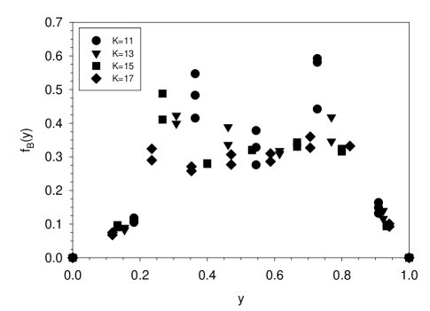
FIG. 1.: The boson structure function $f_{B}$ at various low to moderate numerical resolutions, with $M=\mu$, $\langle:\!\!\phi^{2}(0)\!\!:\rangle=1.0$, $\Lambda^{2}=50\mu^{2}$, $\mu_{1}^{2}=10\mu^{2}$, $\mu_{2}^{2}=20\mu^{2}$, and $\mu_{3}^{2}=30\mu^{2}$. To compare with a structure function computed at higher resolutions, see Fig. 2(d).

Clearly one cure is to work at higher resolution. Limitations on computer storage then require truncation in the number of constituents. Luckily, even at the strongest coupling that we consider, states with large numbers of constituents are unimportant, and yet the results differ significantly from lowest-order perturbation theory. The relative importance of different numbers of constituents can be seen in Table I, where we list probabilities for the various Fock sector contributions to a calculation with moderate resolution. Truncation to a maximum of two bosons is seen to offer a very good approximation. For weaker couplings, lower resolution is sufficient.

TABLE I.: Fock sector probabilities $\int|\phi_{\sigma s}^{(n_{i})}|^{2}\prod_{j}d\underline{q}_{j}$, where $(n_{i})\equiv\{n_{0},n_{1},n_{2},n_{3}\}$, $n=n_{0}$ is the number of physical bosons and $n_{i}$ the number of Pauli–Villars bosons of type $i$. The helicities $\sigma$ and $s$ refer to the physical and bare fermion, respectively. The numerical and physical parameters are $K=17$, $N_{\perp}=5$, $M^{2}=\mu^{2}$, $\Lambda^{2}=50\mu^{2}$, $\mu_{1}^{2}=10\mu^{2}$, $\mu_{2}^{2}=20\mu^{2}$, $\mu_{3}^{2}=30\mu^{2}$, and $\langle:\!\!\phi^{2}(0)\!\!:\rangle=0.5$. Probabilities smaller than $\sim 10^{-5}$ are not resolved with any accuracy.

Number of bosons					Probability			# of
total	$n$	$n_{1}$	$n_{2}$	$n_{3}$	$\sigma=s$	$\sigma=-s$	total	states
0	0	0	0	0	0.9461	—	0.9461	1
1	1	0	0	0	0.0593	0.0444	0.1037	332
1	0	1	0	0	0.0340	0.0571	0.0911	219
1	0	0	1	0	0.0182	0.0300	0.0481	117
1	0	0	0	1	0.0036	0.0044	0.0080	55
2	2	0	0	0	0.0014	0.0021	0.0036	12414
2	1	1	0	0	0.0021	0.0022	0.0043	9969
2	0	2	0	0	0.0006	0.0003	0.0009	1499
2	1	0	1	0	0.0007	0.0007	0.0014	2998
2	0	1	1	0	0.0002	0.0001	0.0003	598
2	0	0	2	0	0.5$\cdot 10^{-5}$	0.4$\cdot 10^{-5}$	0.9$\cdot 10^{-5}$	25
2	1	0	0	1	0.7$\cdot 10^{-4}$	0.7$\cdot 10^{-4}$	0.0001	655
2	0	1	0	1	0.7$\cdot 10^{-5}$	0.6$\cdot 10^{-5}$	0.1$\cdot 10^{-4}$	45
3	3	0	0	0	0.0001	0.2$\cdot 10^{-4}$	0.0001	136568
3	2	1	0	0	0.0002	0.3$\cdot 10^{-4}$	0.0002	102490
3	1	2	0	0	0.6$\cdot 10^{-4}$	0.1$\cdot 10^{-4}$	0.7$\cdot 10^{-4}$	18021
3	0	3	0	0	0.4$\cdot 10^{-5}$	0.1$\cdot 10^{-5}$	0.5$\cdot 10^{-5}$	748
3	2	0	1	0	0.4$\cdot 10^{-4}$	0.6$\cdot 10^{-5}$	0.5$\cdot 10^{-4}$	16631
3	1	1	1	0	0.1$\cdot 10^{-4}$	0.3$\cdot 10^{-5}$	0.2$\cdot 10^{-4}$	2992
3	0	2	1	0	$\sim 10^{-6}$	$\sim 10^{-6}$	$\sim 10^{-6}$	79
4	4	0	0	0	$\sim 10^{-6}$	$\sim 10^{-6}$	$\sim 10^{-6}$	624372
4	3	1	0	0	$\sim 10^{-6}$	$\sim 10^{-6}$	$\sim 10^{-6}$	381016
4	2	2	0	0	$\sim 10^{-6}$	$\sim 10^{-6}$	$\sim 10^{-6}$	57132
4	1	3	0	0	$\sim 10^{-7}$	$\sim 10^{-7}$	$\sim 10^{-7}$	2577
4	0	4	0	0	$\sim 10^{-9}$	$\sim 10^{-9}$	$\sim 10^{-9}$	30
4	3	0	1	0	$\sim 10^{-7}$	$\sim 10^{-6}$	$\sim 10^{-6}$	28613
4	2	1	1	0	$\sim 10^{-7}$	$\sim 10^{-7}$	$\sim 10^{-7}$	2647

Given these considerations for resolution and truncation, we have done two sets of calculations with $K$ between 11 and 29, or even 39. For $K=11$ and 13 there is no explicit truncation and the maximum number of bosons is 5 and 6, respectively. For $K=15$, 17, and 19, the maximum number of bosons used is 4, and for $K\geq 21$ the maximum used is 2. Two different sets of cutoff and PV masses were considered: $\Lambda^{2}=50\mu^{2}$, $\mu_{1}^{2}=10\mu^{2}$, $\mu_{2}^{2}=20\mu^{2}$, and $\mu_{3}^{2}=30\mu^{2}$; and $\Lambda^{2}=100\mu^{2}$, $\mu_{1}^{2}=20\mu^{2}$, $\mu_{2}^{2}=40\mu^{2}$, and $\mu_{3}^{2}=60\mu^{2}$. The transverse resolution $N_{\perp}$ was at least 4 and was increased beyond that to the extent allowed by the available storage on a 16 GB node of an IBM SP. The four processors of the node were used in parallel.

A sampling of explored parameter values can be seen in Tables II-VII. For each choice of input parameter values, these tables present the results for the bare parameters of the Hamiltonian, $g$ and $\delta M^{2}$, and for various expectation values.

TABLE II.: Bare parameters and observables. The input parameter values are $M^{2}=\mu^{2}$, $\Lambda^{2}=50\mu^{2}$, $\mu_{1}^{2}=10\mu^{2}$, $\mu_{2}^{2}=20\mu^{2}$, and $\mu_{3}^{2}=30\mu^{2}$.

$K$	$N_{\perp}$	$\langle:\!\!\phi^{2}(0)\!\!:\rangle$	$g$	$\delta M^{2}/\mu^{2}$	$|\psi_{0}|^{2}$	$-100\mu^{2}F^{\prime}(0)$	$\frac{(\langle y_{1}y_{2}\rangle-\langle y\rangle^{2})_{n\geq 2}}{\langle y\rangle^{2}}$
11	4	0.100	1.279	0.062	0.988	0.090	3653.
11	5	0.100	1.339	0.060	0.989	0.092	3938.
11	6	0.100	1.366	0.066	0.989	0.095	3150.
13	4	0.100	1.274	0.035	0.988	0.092	4117.
13	5	0.100	1.335	0.037	0.989	0.093	3426.
15	4	0.100	1.306	0.084	0.988	0.086	3671.
15	5	0.100	1.361	0.087	0.988	0.091	3108.
17	4	0.100	1.292	0.055	0.988	0.088	3331.
17	5	0.100	1.342	0.055	0.989	0.097	2868.
19	4	0.100	1.287	0.054	0.988	0.091	3324.
19	5	0.100	1.349	0.056	0.988	0.096	3375.
21	4	0.100	1.281	0.055	0.988	0.088	4075.
21	5	0.100	1.350	0.057	0.988	0.095	3257.
21	6	0.100	1.378	0.058	0.989	0.099	2788.
21	7	0.100	1.392	0.058	0.989	0.101	2977.
21	8	0.100	1.400	0.059	0.989	0.104	2920.
29	4	0.100	1.302	0.062	0.987	0.091	3572.
29	5	0.100	1.353	0.063	0.988	0.096	3441.
29	6	0.100	1.386	0.065	0.989	0.099	2920.
29	7	0.100	1.400	0.066	0.989	0.103	2983.

TABLE III.: Additional observables. The input parameter values are the same as for Table II. The dashes represent values not extracted from preliminary, lower-resolution calculations.

$K$	$N_{\perp}$	$\langle:\!\!\phi^{2}(0)\!\!:\rangle$	$\langle n_{B,\sigma}\rangle$	$\langle n_{B,-\sigma}\rangle$	$\langle n_{B}\rangle$	$\langle y_{B,\sigma}\rangle$	$\langle y_{B,-\sigma}\rangle$	$\langle y_{B}\rangle$
11	4	0.100	–	–	0.021	–	–	0.01191
11	5	0.100	–	–	0.021	–	–	0.01209
11	6	0.100	–	–	0.021	–	–	0.01213
13	4	0.100	–	–	0.021	–	–	0.01170
13	5	0.100	–	–	0.022	–	–	0.01219
15	4	0.100	–	–	0.021	–	–	0.01198
15	5	0.100	–	–	0.022	–	–	0.01225
17	4	0.100	–	–	0.022	–	–	0.01220
17	5	0.100	–	–	0.022	–	–	0.01234
19	4	0.100	–	–	0.022	–	–	0.01231
19	5	0.100	–	–	0.022	–	–	0.01238
21	4	0.100	0.0147	0.0072	0.0219	0.00836	0.00417	0.01253
21	5	0.100	0.0133	0.0086	0.0218	0.00735	0.00506	0.01241
21	6	0.100	0.0128	0.0091	0.0220	0.00712	0.00540	0.01252
21	7	0.100	0.0125	0.0094	0.0219	0.00695	0.00556	0.01251
21	8	0.100	0.0125	0.0096	0.0220	0.00691	0.00566	0.01257
29	4	0.100	0.0145	0.0076	0.0221	0.00808	0.00444	0.01252
29	5	0.100	0.0135	0.0086	0.0221	0.00753	0.00508	0.01260
29	6	0.100	0.0129	0.0092	0.0221	0.00711	0.00546	0.01257
29	7	0.100	0.0126	0.0095	0.0221	0.00697	0.00564	0.01261

TABLE IV.: Same as Table II, but for stronger coupling.

$K$	$N_{\perp}$	$\langle:\!\!\phi^{2}(0)\!\!:\rangle$	$g$	$\delta M^{2}/\mu^{2}$	$|\psi_{0}|^{2}$	$-100\mu^{2}F^{\prime}(0)$	$\frac{(\langle y_{1}y_{2}\rangle-\langle y\rangle^{2})_{n\geq 2}}{\langle y\rangle^{2}}$
11	4	1.000	5.417	0.863	0.891	1.340	21.42
11	5	1.001	5.325	0.699	0.899	1.073	27.77
11	6	1.000	5.105	0.819	0.883	2.849	22.06
13	4	1.000	4.520	0.362	0.886	0.929	36.62
13	5	0.998	4.746	0.362	0.893	1.244	28.91
15	4	1.000	5.783	1.161	0.918	0.457	22.85
15	5	1.000	5.589	1.124	0.913	0.641	23.52
17	4	1.000	5.045	0.619	0.909	0.683	25.69
17	5	0.998	4.806	0.562	0.899	1.032	26.31
19	4	1.000	4.804	0.576	0.895	0.853	28.82
19	5	1.000	4.973	0.597	0.902	0.868	29.83
21	4	1.000	4.925	0.615	0.896	0.774	32.23
21	5	1.000	5.082	0.616	0.903	0.876	28.27
21	6	1.000	4.978	0.619	0.900	1.266	25.64
21	7	0.999	5.046	0.612	0.903	1.140	27.78
21	8	1.000	5.009	0.622	0.901	1.248	27.68
29	4	1.000	5.089	0.713	0.902	0.659	29.23
29	5	1.000	5.072	0.695	0.901	0.837	29.11
29	6	1.000	5.173	0.708	0.907	0.867	26.29
29	7	0.999	5.152	0.712	0.905	0.933	27.62

TABLE V.: Same as Table III, but for stronger coupling.

$K$	$N_{\perp}$	$\langle:\!\!\phi^{2}(0)\!\!:\rangle$	$\langle n_{B,\sigma}\rangle$	$\langle n_{B,-\sigma}\rangle$	$\langle n_{B}\rangle$	$\langle y_{B,\sigma}\rangle$	$\langle y_{B,-\sigma}\rangle$	$\langle y_{B}\rangle$
11	4	1.000	–	–	0.237	–	–	0.1425
11	5	1.001	–	–	0.231	–	–	0.1342
11	6	1.000	–	–	0.233	–	–	0.1383
13	4	1.000	–	–	0.217	–	–	0.1205
13	5	0.998	–	–	0.222	–	–	0.1280
15	4	1.000	–	–	0.210	–	–	0.1167
15	5	1.000	–	–	0.212	–	–	0.1181
17	4	1.000	–	–	0.211	–	–	0.1192
17	5	0.998	–	–	0.214	–	–	0.1212
19	4	1.000	–	–	0.216	–	–	0.1220
19	5	1.000	–	–	0.216	–	–	0.1217
21	4	1.000	0.1179	0.0994	0.2173	0.06625	0.05649	0.12275
21	5	1.000	0.1044	0.1129	0.2174	0.05788	0.06580	0.12368
21	6	1.000	0.1031	0.1154	0.2185	0.05770	0.06759	0.12529
21	7	1.000	0.1008	0.1162	0.2170	0.05575	0.06751	0.12326
21	8	1.000	0.1016	0.1153	0.2169	0.05608	0.06655	0.12263
29	4	1.000	0.1088	0.1057	0.2145	0.05894	0.06072	0.11966
29	5	1.000	0.1048	0.1122	0.2170	0.05738	0.06452	0.12190
29	6	1.000	0.0982	0.1178	0.2160	0.05363	0.06824	0.12187
29	7	1.000	0.0985	0.1180	0.2165	0.05360	0.06803	0.12163

TABLE VI.: Same as Table IV, but for $\Lambda^{2}=100\mu^{2}$, $\mu_{1}^{2}=20\mu^{2}$, $\mu_{2}^{2}=40\mu^{2}$, and $\mu_{3}^{2}=60\mu^{2}$.

$K$	$N_{\perp}$	$\langle:\!\!\phi^{2}(0)\!\!:\rangle$	$g$	$\delta M^{2}/\mu^{2}$	$|\psi_{0}|^{2}$	$-100\mu^{2}F^{\prime}(0)$	$\frac{(\langle y_{1}y_{2}\rangle-\langle y\rangle^{2})_{n\geq 2}}{\langle y\rangle^{2}}$
11	4	0.989	4.661	1.220	0.858	1.195	22.07
11	5	0.998	4.326	0.991	0.868	1.114	26.07
11	6	0.904	4.181	1.063	0.882	1.442	28.64
13	4	1.002	3.378	0.487	0.836	1.122	32.87
13	5	1.000	4.182	0.537	0.863	1.245	27.45
15	4	1.000	5.332	1.849	0.912	0.337	19.69
15	5	1.000	5.142	1.804	0.908	0.458	21.64
17	4	0.998	4.448	1.131	0.896	0.448	28.27
17	5	1.000	4.527	1.094	0.889	0.758	24.09
19	4	1.000	4.317	0.915	0.873	0.759	27.20
19	5	0.999	4.412	0.970	0.880	0.960	24.52
21	4	1.000	4.300	0.966	0.876	0.752	25.75
29	4	1.000	4.795	1.160	0.886	0.565	23.4
29	5	0.999	4.683	1.132	0.893	0.699	22.5
29	6	1.000	4.772	1.164	0.897	0.757	21.9
29	7	0.999	4.706	1.160	0.893	1.079	20.9
39	4	0.998	4.562	1.006	0.884	0.660	23.6
39	5	1.000	4.678	1.026	0.892	0.729	22.3
39	6	1.000	4.656	1.020	0.894	0.833	21.8

TABLE VII.: Same as Table V, but for $\Lambda^{2}=100\mu^{2}$, $\mu_{1}^{2}=20\mu^{2}$, $\mu_{2}^{2}=40\mu^{2}$, and $\mu_{3}^{2}=60\mu^{2}$.

$K$	$N_{\perp}$	$\langle:\!\!\phi^{2}(0)\!\!:\rangle$	$\langle n_{B,\sigma}\rangle$	$\langle n_{B,-\sigma}\rangle$	$\langle n_{B}\rangle$	$\langle y_{B,\sigma}\rangle$	$\langle y_{B,-\sigma}\rangle$	$\langle y_{B}\rangle$
11	4	0.989	–	–	0.245	–	–	0.1524
11	5	0.998	–	–	0.227	–	–	0.1310
11	6	0.904	–	–	0.206	–	–	0.1207
13	4	1.002	–	–	0.228	–	–	0.1297
13	5	1.000	–	–	0.230	–	–	0.1370
15	4	1.000	–	–	0.205	–	–	0.1149
15	5	1.000	–	–	0.204	–	–	0.1140
17	4	0.998	–	–	0.198	–	–	0.1078
17	5	1.000	–	–	0.212	–	–	0.1203
19	4	1.000	–	–	0.218	–	–	0.1261
19	5	0.999	–	–	0.218	–	–	0.1271
21	4	1.000	–	–	0.215	–	–	0.1245
29	4	1.000	0.1051	0.1152	0.2203	0.06028	0.06653	0.12680
29	5	1.000	0.0894	0.1231	0.2125	0.04925	0.07260	0.12185
29	6	1.000	0.0798	0.1317	0.2115	0.04334	0.07794	0.12128
29	7	1.000	0.0787	0.1350	0.2137	0.04357	0.08055	0.12412
39	4	1.000	0.1069	0.1090	0.2159	0.06156	0.06396	0.12552
39	5	1.000	0.0907	0.1232	0.2139	0.05109	0.07272	0.12381
39	6	1.000	0.0836	0.1297	0.2133	0.04611	0.07694	0.12305

For higher resolution ($K=21$ and 29 for $\Lambda^{2}=50\mu^{2}$ and $K=29$ and 39 for $\Lambda^{2}=100\mu^{2}$) we plot the structure function $f_{B}$ in Figs. 2 and 3. Typical contributions to $f_{B}$ from one-boson and two-boson states are shown in Fig. 4. The two-boson contribution to the structure function is further analyzed in terms of its dependence on both longitudinal momentum fractions in Fig. 5, where

$$\tilde{f}_{B\sigma}(y_{1},y_{2})\equiv\int d^{2}q_{\perp 1}d^{2}q_{\perp 2}|\phi_{\sigma\sigma}^{(2,0,0,0)}(\underline{q}_{j})|^{2}$$ (36)

is plotted. We also show typical two-body wave functions in Fig. 6; the agreement with the necessary $L_{z}=1$ symmetry in the antiparallel helicity case is an important check of $J_{z}$ conservation in the calculation.

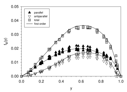
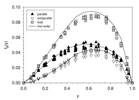
(a)	(b)
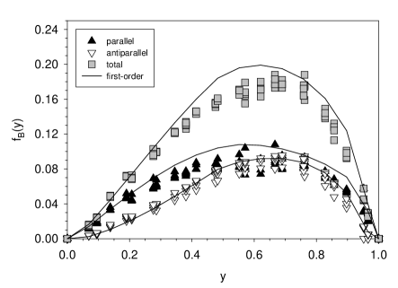
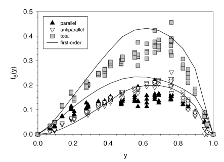
(c)	(d)

FIG. 2.: The boson structure function $f_{B}$ at various numerical resolutions for (a) $\langle:\!\!\phi^{2}(0)\!\!:\rangle=0.1$, (b) $\langle:\!\!\phi^{2}(0)\!\!:\rangle=0.25$, (c) $\langle:\!\!\phi^{2}(0)\!\!:\rangle=0.5$, and (d) $\langle:\!\!\phi^{2}(0)\!\!:\rangle=1.0$, with $M=\mu$, $\Lambda^{2}=50\mu^{2}$, $\mu_{1}^{2}=10\mu^{2}$, $\mu_{2}^{2}=20\mu^{2}$, and $\mu_{3}^{2}=30\mu^{2}$. The solid line is from first-order perturbation theory.

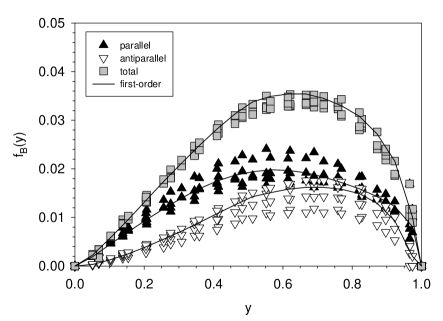
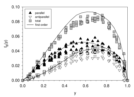
(a)	(b)
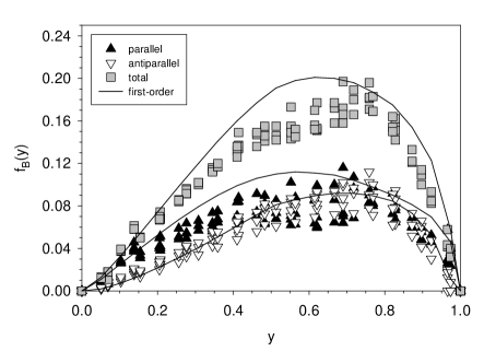
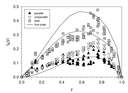
(c)	(d)

FIG. 3.: Same as Fig. 2 but for $\Lambda^{2}=100\mu^{2}$, $\mu_{1}^{2}=20\mu^{2}$, $\mu_{2}^{2}=40\mu^{2}$, and $\mu_{3}^{2}=60\mu^{2}$.

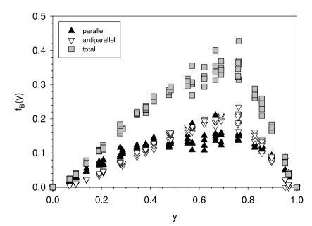
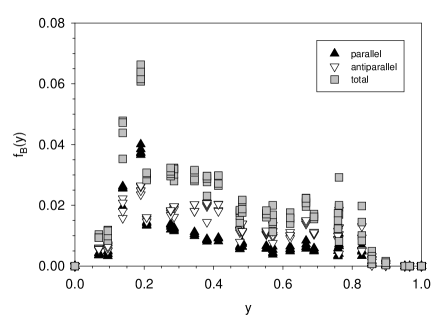
(a)	(b)

FIG. 4.: The (a) one-boson and (b) two-boson contributions to the boson structure function $f_{B}$ at various numerical resolutions, with $M=\mu$, $\langle:\!\!\phi^{2}(0)\!\!:\rangle=1$, $\Lambda^{2}=50\mu^{2}$, $\mu_{1}^{2}=10\mu^{2}$, $\mu_{2}^{2}=20\mu^{2}$, and $\mu_{3}^{2}=30\mu^{2}$.

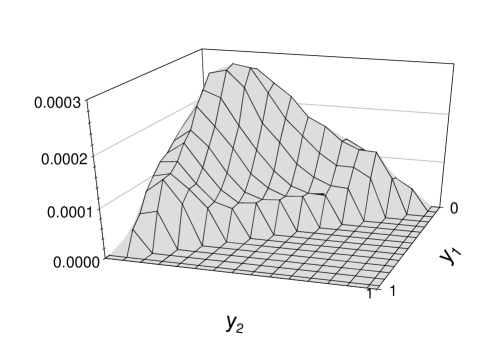
FIG. 5.: The two-boson structure function $\tilde{f}_{B\sigma}$ for $K=29$ and $N_{\perp}=7$, with $M=\mu$, $\langle:\!\!\phi^{2}(0)\!\!:\rangle=1$, $\Lambda^{2}=50\mu^{2}$, $\mu_{1}^{2}=10\mu^{2}$, $\mu_{2}^{2}=20\mu^{2}$, and $\mu_{3}^{2}=30\mu^{2}$.

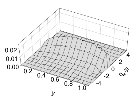
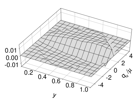
(a)	(b)

FIG. 6.: The one-boson amplitude $\phi_{\sigma s}^{(1,0,0,0)}$, with (a) parallel ($s=\sigma$) and (b) antiparallel ($s=-\sigma$) bare helicity, as a function of longitudinal momentum fraction $y$ and one transverse momentum component $q_{x}$ in the $q_{y}=0$ plane. The parameter values are $K=29$, $N_{\perp}=7$, $M=\mu$, $\Lambda^{2}=50\mu^{2}$, $\mu_{1}^{2}=10\mu^{2}$, $\mu_{2}^{2}=20\mu^{2}$, $\mu_{3}^{2}=30\mu^{2}$, and $\langle:\!\!\phi^{2}(0)\!\!:\rangle=0.25$.

As a check on the logarithmic PV coupling constraint in Eq. (14), we compute the bare mass shift $\delta M^{2}$ when $M^{2}$ is much less than $\mu^{2}$. Figure 7 shows its behavior as a function of the longitudinal resolution for various bare couplings. If the logarithmic constraint was sufficient for nonperturbative calculation, $\delta M^{2}$ should go to zero as $M^{2}$ approaches zero and the resolution approaches the continuum limit. This appears to work well only for weak coupling.

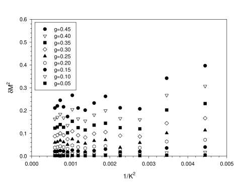
FIG. 7.: The bare mass shift $\delta M^{2}$ as a function of the longitudinal resolution $K$ for various bare couplings $g$, with $N_{\perp}=4$, $M^{2}=0.001\mu^{2}$, $\Lambda^{2}=50\mu^{2}$, $\mu_{1}^{2}=10\mu^{2}$, $\mu_{2}^{2}=20\mu^{2}$, and $\mu_{3}^{2}=30\mu^{2}$.

IV Conclusions and Prospects for the Application of DLCQ(3+1) to Gauge Theory

We have used the discretized light-cone quantization method to successfully solve for the mass and light-cone wave functions of a dressed fermionic state in a Yukawa theory in $3+1$ space-time dimensions. No a priori constraint on the number of bosonic constituents was necessary; however, since the fermion constituent was treated as heavy, states containing fermion–anti-fermion pairs were truncated. We have found that the eigensolution at strong coupling displays features which significantly deviated from first-order perturbation theory. Numerical resolution in this domain of strong coupling was not a limiting factor in this analysis.

The regularization procedure which we have chosen, with three PV scalars, functioned well. However, better convergence of the DLCQ method at strong coupling could be obtained by constraining the PV couplings non-perturbatively, rather than using the one-loop perturbative constraints in (14).

A number of properties of the Yukawa-theory eigensolution could be extracted from its light-cone Fock-state wave function. This illustrates the power of the DLCQ method in making the Fock-state wave functions of the eigenstates explicitly available. It is also possible to use the derived wave functions to compute the Pauli and Dirac form factors of the dressed fermion state at general momentum transfers [29].

There are additional calculations which might be done within the context of the zero fermion pair approximation. We could consider two-fermion states and study true bound states and scattering solutions. We could also consider dressed spin-3/2 states and the analog of N$\pi\leftrightarrow\Delta$ transitions. Extension of these methods to pseudo-scalar Yukawa theory would make the N$\pi\leftrightarrow\Delta$ connection stronger.

Although the approach used in this paper to solve (3+1)-dimensional Yukawa theory at strong coupling has been successful, future progress for solving other quantum field theories will require more efficient analytic methods and numerical algorithms. An alternative ultraviolet regularization procedure, using only one PV scalar and one PV fermion [30, 28] may potentially provide a more efficient approach for solving Yukawa theories. Not only is the constraint on the couplings trivial, but the light-cone Hamiltonian is also much simpler. The simplifications occur because the instantaneous fermion interactions (the terms in (9) of order $g^{2}$) cancel. Moreover, the DLCQ matrix for the remaining three-point interactions is much more sparse, allowing calculations at higher resolutions. Our next step will be to test this alternative regularization.

One can consider two other possibilities for PV regularization [30] of full Yukawa theory. One is to use two heavy fermions and one heavy scalar [23]; the other is to use one less heavy fermion but make the transverse momentum cutoff part of the regularization rather than just a numerical procedure. In each case a $\phi^{4}$ term must be added. We plan to explore both of these methods.

Quantum electrodynamics and quantum chromodynamics in physical space-time, including the phenomenon of chiral symmetry breaking remain the central challenge to DLCQ methods. One attractive possible approach is to use broken supersymmetry as an effective ultraviolet regulator of the light-cone Hamiltonians of gauge theories.

The PV method also has applicability to the renormalization of non-Abelian Hamiltonian gauge theories on the light-cone. Paston, Franke and Prokhvatilov [31, 32] have recently extended their analysis to the nonperturbative regulation of light-cone QCD, including the regularization of the infrared singularities introduced by using light-cone gauge. They find that a combination of light-cone gauge, PV fields, higher derivative regulation, and carefully chosen momentum cutoffs can regulate the theory in such a way as to provide agreement with Feynman calculations using the Mandelstam–Leibbrandt prescription [33] for the spurious singularity in the gauge propagator. The resulting dynamical operator is rather complex and several regulating fields are needed, but the regulation procedures appear suitable for numerical calculations. We plan to test these methods in Abelian theory, including the calculation of positronium bound states [34, 35] and the non-perturbative calculation of the anomalous magnetic moments of leptons at strong coupling [36].

Lanczos algorithm for indefinite metric

The ordinary Lanczos algorithm [27] was designed for diagonalization of real symmetric or Hermitian matrices. A more general form, the biorthogonal Lanczos algorithm [37], can be applied to non-symmetric cases but is quite cumbersome. In the case of a complex symmetric matrix, the biorthogonal algorithm can be reduced to a form nearly as simple as the real symmetric case [38]; this approach was used in previous work [18, 21] where imaginary couplings made negative norms unnecessary. The complex-symmetric approach is not easy to implement for Yukawa theory because the Hamiltonian is fully Hermitian. Instead, negative norms are assigned, and the eigenvalue problem becomes one with indefinite metric.

For this case the biorthogonal algorithm can still be reduced to a simpler form. Let $\eta$ represent the metric signature, so that numerical dot products are written $\langle\phi^{\prime}|\phi\rangle={\mathchoice{{\hbox{\boldmath$\displaystyle\phi$}}}{{\hbox{\boldmath$\textstyle\phi$}}}{{\hbox{\boldmath$\scriptstyle\phi$}}}{{\hbox{\boldmath$\scriptscriptstyle\phi$}}}}^{\,\prime*}\cdot\eta{\mathchoice{{\hbox{\boldmath$\displaystyle\phi$}}}{{\hbox{\boldmath$\textstyle\phi$}}}{{\hbox{\boldmath$\scriptstyle\phi$}}}{{\hbox{\boldmath$\scriptscriptstyle\phi$}}}}$. The Hamiltonian matrix $H$ is constructed to be self-adjoint with respect to this metric, which means that [39] $\bar{H}\equiv\eta^{-1}H^{\dagger}\eta=H$. The Lanczos algorithm for the diagonalization of $H$ then takes the form

$$\alpha_{j} = \nu_{j}{\mathchoice{{\hbox{\boldmath$\displaystyle q$}}}{{\hbox{\boldmath$\textstyle q$}}}{{\hbox{\boldmath$\scriptstyle q$}}}{{\hbox{\boldmath$\scriptscriptstyle q$}}}}_{j}^{\,*}\cdot\eta H{\mathchoice{{\hbox{\boldmath$\displaystyle q$}}}{{\hbox{\boldmath$\textstyle q$}}}{{\hbox{\boldmath$\scriptstyle q$}}}{{\hbox{\boldmath$\scriptscriptstyle q$}}}}_{j}\,,\;\;{\mathchoice{{\hbox{\boldmath$\displaystyle r$}}}{{\hbox{\boldmath$\textstyle r$}}}{{\hbox{\boldmath$\scriptstyle r$}}}{{\hbox{\boldmath$\scriptscriptstyle r$}}}}_{j}=H{\mathchoice{{\hbox{\boldmath$\displaystyle q$}}}{{\hbox{\boldmath$\textstyle q$}}}{{\hbox{\boldmath$\scriptstyle q$}}}{{\hbox{\boldmath$\scriptscriptstyle q$}}}}_{j}-\gamma_{j-1}{\mathchoice{{\hbox{\boldmath$\displaystyle q$}}}{{\hbox{\boldmath$\textstyle q$}}}{{\hbox{\boldmath$\scriptstyle q$}}}{{\hbox{\boldmath$\scriptscriptstyle q$}}}}_{j-1}-\alpha_{j}{\mathchoice{{\hbox{\boldmath$\displaystyle q$}}}{{\hbox{\boldmath$\textstyle q$}}}{{\hbox{\boldmath$\scriptstyle q$}}}{{\hbox{\boldmath$\scriptscriptstyle q$}}}}_{j}\,,\;\;\beta_{j}=+\sqrt{|{\mathchoice{{\hbox{\boldmath$\displaystyle r$}}}{{\hbox{\boldmath$\textstyle r$}}}{{\hbox{\boldmath$\scriptstyle r$}}}{{\hbox{\boldmath$\scriptscriptstyle r$}}}}_{j}^{\,*}\cdot\eta{\mathchoice{{\hbox{\boldmath$\displaystyle r$}}}{{\hbox{\boldmath$\textstyle r$}}}{{\hbox{\boldmath$\scriptstyle r$}}}{{\hbox{\boldmath$\scriptscriptstyle r$}}}}_{j}|}\,,\;\;$$ (37)

$${\mathchoice{{\hbox{\boldmath$\displaystyle q$}}}{{\hbox{\boldmath$\textstyle q$}}}{{\hbox{\boldmath$\scriptstyle q$}}}{{\hbox{\boldmath$\scriptscriptstyle q$}}}}_{j+1} = {\mathchoice{{\hbox{\boldmath$\displaystyle r$}}}{{\hbox{\boldmath$\textstyle r$}}}{{\hbox{\boldmath$\scriptstyle r$}}}{{\hbox{\boldmath$\scriptscriptstyle r$}}}}_{j}/\beta_{j}\,,\;\;\nu_{j+1}=\mbox{sign}({\mathchoice{{\hbox{\boldmath$\displaystyle r$}}}{{\hbox{\boldmath$\textstyle r$}}}{{\hbox{\boldmath$\scriptstyle r$}}}{{\hbox{\boldmath$\scriptscriptstyle r$}}}}_{j}^{\,*}\cdot\eta{\mathchoice{{\hbox{\boldmath$\displaystyle r$}}}{{\hbox{\boldmath$\textstyle r$}}}{{\hbox{\boldmath$\scriptstyle r$}}}{{\hbox{\boldmath$\scriptscriptstyle r$}}}}_{j})\,,\;\;\nu_{1}=\mbox{sign}({\mathchoice{{\hbox{\boldmath$\displaystyle q$}}}{{\hbox{\boldmath$\textstyle q$}}}{{\hbox{\boldmath$\scriptstyle q$}}}{{\hbox{\boldmath$\scriptscriptstyle q$}}}}_{1}^{\,*}\cdot\eta{\mathchoice{{\hbox{\boldmath$\displaystyle q$}}}{{\hbox{\boldmath$\textstyle q$}}}{{\hbox{\boldmath$\scriptstyle q$}}}{{\hbox{\boldmath$\scriptscriptstyle q$}}}}_{1})\,,\;\;\gamma_{j}=\nu_{j+1}\nu_{j}\beta_{j}\,,$$ (38)

where ${\mathchoice{{\hbox{\boldmath$\displaystyle q$}}}{{\hbox{\boldmath$\textstyle q$}}}{{\hbox{\boldmath$\scriptstyle q$}}}{{\hbox{\boldmath$\scriptscriptstyle q$}}}}_{1}$ is taken as a normalized initial guess and $\gamma_{0}=0$. This initial guess is generated with use of high-order Brillouin–Wigner perturbation theory. To determine when to stop the Lanczos iterations, the convergence of the eigenvalue and parts of the boson-fermion wave function are monitored.

Just as for the ordinary Lanczos algorithm, the original matrix $H$ acquires the following tridiagonal matrix representation $T$ with respect to the basis formed by the vectors ${\mathchoice{{\hbox{\boldmath$\displaystyle q$}}}{{\hbox{\boldmath$\textstyle q$}}}{{\hbox{\boldmath$\scriptstyle q$}}}{{\hbox{\boldmath$\scriptscriptstyle q$}}}}_{j}$:

$$H\rightarrow T\equiv\left(\begin{array}[]{llllll}\alpha_{1}&\beta_{1}&0&0&0&\ldots\\ \gamma_{1}&\alpha_{2}&\beta_{2}&0&0&\ldots\\ 0&\gamma_{2}&\alpha_{3}&\beta_{3}&0&\ldots\\ 0&0&\gamma_{3}&.&.&\ldots\\ 0&0&0&.&.&\ldots\\ .&.&.&.&.&\ldots\end{array}\right)\,.$$ (39)

By construction, the elements of $T$ are real. The new matrix is also self-adjoint, but with respect to an induced metric $\nu=\{\nu_{1},\nu_{2},\ldots\}$. The eigenvalues of $T$ approximate some of the eigenvalues of $H$, even after only a few iterations. Approximate eigenvectors of $H$ are constructed from the right eigenvectors ${\mathchoice{{\hbox{\boldmath$\displaystyle c$}}}{{\hbox{\boldmath$\textstyle c$}}}{{\hbox{\boldmath$\scriptstyle c$}}}{{\hbox{\boldmath$\scriptscriptstyle c$}}}}_{i}$ of $T$ as ${\mathchoice{{\hbox{\boldmath$\displaystyle\phi$}}}{{\hbox{\boldmath$\textstyle\phi$}}}{{\hbox{\boldmath$\scriptstyle\phi$}}}{{\hbox{\boldmath$\scriptscriptstyle\phi$}}}}_{i}=\sum_{k}(c_{i})_{k}{\mathchoice{{\hbox{\boldmath$\displaystyle q$}}}{{\hbox{\boldmath$\textstyle q$}}}{{\hbox{\boldmath$\scriptstyle q$}}}{{\hbox{\boldmath$\scriptscriptstyle q$}}}}_{k}$.

REFERENCES

- [1] H.-C. Pauli and S.J. Brodsky, Phys. Rev. D 32, 1993 (1985); 32, 2001 (1985).
- [2] For reviews, see S.J. Brodsky and H.-C. Pauli, in Recent Aspects of Quantum Fields, edited by H. Mitter and H. Gausterer, Lecture Notes in Physics Vol. 396 (Springer-Verlag, Berlin, 1991); S.J. Brodsky, G. McCartor, H.-C. Pauli, and S.S. Pinsky, Part. World 3, 109 (1993); M. Burkardt, Adv. Nucl. Phys. 23, 1 (1996); S.J. Brodsky, H.-C. Pauli, and S.S. Pinsky, Phys. Rep. 301, 299 (1997), hep-ph/9705477.
- [3] S.J. Brodsky, “QCD aspects of exclusive B decays,” hep-ph/0104153.
- [4] M. Beneke, G. Buchalla, M. Neubert, and C.T. Sachrajda, Nucl. Phys. B 591, 313 (2000), hep-ph/0006124.
- [5] Y.-Y. Keum, H.-N. Li, and A. I. Sanda, Phys. Rev. D 63, 054008 (2001), hep-ph/0004173.
- [6] S.J. Brodsky and D.S. Hwang, Nucl. Phys. B 543, 239 (1999), hep-ph/9806358.
- [7] S.J. Brodsky, M. Diehl, and D.S. Hwang, Nucl. Phys. B 596, 99 (2001), hep-ph/0009254.
- [8] M. Diehl, T. Feldmann, R. Jakob, and P. Kroll, Nucl. Phys. B 596, 33 (2001), hep-ph/0009255; 605, 647 (2001).
- [9] For a review, see S.J. Brodsky, “Hadronic light-front wave functions and QCD phenomenology,” hep-ph/0102051.
- [10] O. Lunin and S. Pinsky, Phys. Rev. D 63, 045019 (2001), hep-th/0005282.
- [11] D.J. Gross, A. Hashimoto, and I.R. Klebanov, Phys. Rev. D 57, 6420 (1998), hep-th/9710240.
- [12] F. Antonuccio, O. Lunin, S. Pinsky, and A. Hashimoto, JHEP 07, 029 (1999); J.R. Hiller, O. Lunin, S. Pinsky, and U. Trittmann, Phys. Lett. B 482, 409 (2000); J.R. Hiller, S. Pinsky, and U. Trittmann, Phys. Rev. D 63, 105017 (2001).
- [13] F. Antonuccio and S.S. Pinsky, Phys. Lett. B 397, 42 (1997), hep-th/9612021.
- [14] W.A. Bardeen and R. Pearson, Phys. Rev. D 14, 547 (1976); W.A. Bardeen, R.B. Pearson, and E. Rabinovici, ibid. 21, 1037 (1980); P.A. Griffin, Mod. Phys. Lett. A 7, 601 (1992); Nucl. Phys. B372, 270 (1992); Phys. Rev. D 46, 3538 (1992); 47, 3530 (1993); M. Burkardt, ibid. 47, 4628 (1993); 49, 5446 (1994); M. Burkardt, in the proceedings of the 1995 ELFE Summer School and Workshop, Confinement Physics, edited by S. Bass and P.A.M. Guichon, (Gif-sur-Yvette, Ed. Frontieres, 1996), p. 255; M. Burkardt and B. Klindworth, Phys. Rev. D 55, 1001 (1997); S. Dalley and B. van de Sande, ibid. 59, 065008 (1999); 63, 076004 (2001).
- [15] S. Dalley, Phys. Rev. D 64, 036006 (2001), hep-ph/0101318.
- [16] S.K. Seal and M. Burkardt, Nucl. Phys. B (Proc. Suppl.) 90, 233 (2000).
- [17] M. Burkardt and S.K. Seal, hep-ph/0105109.
- [18] S.J. Brodsky, J.R. Hiller, and G. McCartor, Phys. Rev. D 58, 025005 (1998).
- [19] W. Pauli and F. Villars, Rev. Mod. Phys. 21, 4334 (1949).
- [20] K.R. Dienes, Nucl. Phys. B 611, 146 (2001), hep-ph/0104274.
- [21] S.J. Brodsky, J.R. Hiller, and G. McCartor, Phys. Rev. D 60, 054506 (1999).
- [22] S.A. Paston and V.A. Franke, Theor. Math. Phys. 112, 1117 (1997), hep-th/9901110.
- [23] S.A. Paston, E.V. Prokhvatilov, and V.A. Franke, hep-th/9910114.
- [24] P.A.M. Dirac, Rev. Mod. Phys. 21, 392 (1949).
- [25] G. McCartor and D.G. Robertson, Z. Phys. C 53, 679 (1992).
- [26] C. Bouchiat, P. Fayet, and N. Sourlas, Lett. Nuovo Cim. 4, 9 (1972); S.-J. Chang and T.-M. Yan, Phys. Rev. D 7, 1147 (1973); M. Burkardt and A. Langnau, Phys. Rev. D 44, 3857 (1991).
- [27] C. Lanczos, J. Res. Nat. Bur. Stand. 45, 255 (1950); J.H. Wilkinson, The Algebraic Eigenvalue Problem (Clarendon, Oxford, 1965); B.N. Parlett, The Symmetric Eigenvalue Problem (Prentice–Hall, Englewood Cliffs, NJ, 1980); J. Cullum and R.A. Willoughby, J. Comput. Phys. 44, 329 (1981); Lanczos Algorithms for Large Symmetric Eigenvalue Computations (Birkhauser, Boston, 1985), Vols. I and II; G.H. Golub and C.F. van Loan, Matrix Computations (Johns Hopkins University Press, Baltimore, 1983).
- [28] S.J. Brodsky, J.R. Hiller, and G. McCartor, submitted to Phys. Rev. D, hep-th/0107246.
- [29] J.R. Hiller, in the proceedings of the Workshop on the Transition from Low to High Q Form Factors, (TJNAF, Newport News, VA, 1999), p. 193, hep-ph/9909471.
- [30] S.A. Paston, V.A. Franke, and E.V. Prokhvatilov, private communication.
- [31] S.A. Paston, V.A. Franke, and E.V. Prokhvatilov, Theor. Math. Phys. 120, 1164 (1999) [Teor. Mat. Fiz. 120, 417 (1999)], hep-th/0002062.
- [32] S.A. Paston, E.V. Prokhvatilov, and V.A. Franke, hep-th/0011224.
- [33] S. Mandelstam, Nucl. Phys. B213, 149 (1983); G. Leibbrandt, Phys. Rev. D 29, 1699 (1984).
- [34] M. Krautgartner, H.-C. Pauli, and F. Wolz, Phys. Rev. D 45, 3755 (1992).
- [35] M. Kaluza and H. C. Pauli, Phys. Rev. D 45, 2968 (1992).
- [36] J.R. Hiller and S.J. Brodsky, Phys. Rev. D 59, 016006 (1999).
- [37] J.H. Wilkinson, Ref. REFERENCES; Y. Saad, Comput. Phys. Commun. 53, 71 (1989); S.K. Kin and A.T. Chronopoulos, J. Comp. and Appl. Math 42, 357 (1992).
- [38] J. Cullum and R.A. Willoughby, in Large-Scale Eigenvalue Problems, eds. J. Cullum and R.A. Willoughby, Math. Stud. 127 (Elsevier, Amsterdam, 1986), p. 193.
- [39] W. Pauli, Rev. Mod. Phys. 15, 175 (1943).