Probing an extended region of $\Delta m^{2}$ with rapidly oscillating ⁷Be solar neutrinos

Abstract

If ⁷Be solar neutrinos can be observed in real time experiments, then an extended region of $\Delta m^{2}$ can be probed by a proper analysis of the rapidly changing phase of vacuum oscillations due to the eccentricity of the earth’s orbit about the sun. For the case of maximal vacuum mixing, a kind of Fourier analysis of expected data for one year’s time could uniquely pick out $\Delta m^{2}$ if it lies in the region $\sim 10^{-10}-6\times 10^{-9}$(eV)².
PACS: 14.60.Pq, 13.10.+q, 25.30.Pt

I Introduction

In a previous work it was argued[1] that with maximal vacuum mixing there is agreement, with minor modifications, between extant observations of solar neutrinos and predictions by the standard solar model (SSM)[2, 3, 4, 5]. The maximal vacuum mixing case considered was that in which the phase of neutrino oscillations coming from the sun is averaged, leading to $50\%$ of the neutrinos arriving at the earth as electron neutrinos. As a result of this averaging, while $\sin^{2}2\theta$ was assumed to be maximal (equal to one), $\Delta m^{2}$ was not determined and taken to lie in the approximate range $10^{-9}<\Delta m^{2}<<10^{-3}$ with an exclusion of the approximate range $3\times 10^{-7}<\Delta m^{2}<10^{-5}$ for maximal mixing[6] due to the lack of an observed day-night effect in the SuperKamiokande data[7].

On the other hand, the recent first results of the SNO measurement of charged current interactions produced by ⁸B neutrinos[8], taken in combination with the elastic scattering result of the Super-Kamiokande collaboration[7], indicate that only about one third of the neutrinos arriving at the earth from the sun are electron neutrinos, with the other two thirds being $\mu$ or $\tau$ neutrinos. Oscillation into sterile neutrinos now seems relatively unlikely from the SNO result.

While at first glance this comparison seems to make maximal vacuum mixing less likely, a global analysis of the SNO result with the other solar neutrino experiments, chlorine[9], Super-Kamiokande[7], and gallium[10, 11] has led to the conclusion that “the CC measurement by SNO has not changed qualitatively the globally allowed solution space for solar neutrinos, although the CC measurement has provided dramatic and convincing evidence for neutrino oscillations and has strenghened the ths case for active oscillations with large mixing angles[12].” Furthermore, global analyses[12][13] do not completely exclude solutions to the solar neutrino problem in the mass region $10^{-10}<\Delta m^{2}<10^{-8}$ for maximal (or near maximal) mixing. In the following, the time varying phase of oscillating ⁷Be neutrinos is investigated as a possible method to discover (or exclude) a solution of the solar neutrino problem in that mass region.

In the mass region $4\times 10^{-11}<\Delta m^{2}<10^{-9}$ there are so-called “just-so” vacuum solutions of the solar neutrino problem, where the phase of the oscillation of ⁸B neutrinos coming from the sun is not completely averaged[14, 15]. Recall also[16, 17], that there is a large change in the ⁷Be electron neutrino flux over the year in the ⁸B “just-so” region due to the change in phase of order $\pi/2$ in a year brought about by the $\pm 1.67\%$ yearly orbital variation from the mean distance of the sun to the earth. As will be shown in the following, when phase averaging due to the temperature of the sun and phase damping due to the MSW effect are considered, it turns out that phase variation in ⁷Be neutrinos should be observable for $\Delta m^{2}$ in the range from about $10^{-10}$ up to about $6\times 10^{-9}$ (eV)². This observable range of $\Delta m^{2}$ via ⁷Be neutrinos turns out to be in approximate agreement with a previous analysis by de Gouvêa, Friedland, and Murayama[18].

II Oscillations: thermal averaging; MSW damping

There is a low energy region of solar neutrinos dominated by the nearly monenergetic 862 KeV line from electron capture by ⁷Be in the sun. It is the purpose of the Borexino[19] experiment, soon to come on line, to measure these neutrinos in real time. Feasability studies are also being carried out for other experiments to measure ⁷Be neutrinos in real time such as LENS[20] and HELLAZ[21].

If the ⁷Be neutrinos were truly monoenergetic then the number of neutrinos detected via electron scattering in an experiment like Borexino (normalized to unity for no oscillations) would take the following form for vacuum oscillations

$$R(\phi,\Delta m^{2})=1-0.79\sin^{2}2\theta\sin^{2}{\pi\Delta m^{2}L(\phi)\over(0.862)0.00248},$$ (1)

where $\theta$ is the vacuum mixing angle, $\Delta m^{2}$ is expressed in (eV)², the $\mu$ or $\tau$ neutrino scattering relative to electron neutrino scattering at 0.862 MeV is 0.21[22], and

$$L(\phi)={1-\epsilon^{2}\over 1+\epsilon\cos{\phi}}1.496\times 10^{8},$$ (2)

the distance from the Earth to the center of the sun (in km.), which varies through the year due to the eccentricity $\epsilon=.0167$ of the Earth’s orbit about the sun. Note that since we take the number of neutrinos detected as a function of $\phi$, the phase of the earth in its orbit about the sun, rather than of the time of the year there is no $1/L^{2}$ seasonal variation in $R$; it is canceled by the Jacobian in going from time as an independent variable to $\phi$ as an independent variable (Kepler’s second law).

It has been pointed out by Pakvasa and Pantaleone[23] that the ⁷Be energy line is thermally broadened not only by the spread in nuclear velocities (Doppler broadening) but also by the solar temperature of the approximately 80% of the capture electrons that come from the continuum. We makes use of the published table of Bahcall [24] which was obtained by convoluting both these sources of thermal spreading to obtain the energy profile of the 862 keV ⁷Be solar neutrino shown in Figure 1. Note that the distribution $w_{t}(x)$ is asymmetric in shape and plotted as a function of $x=(E-0.862)/0.862$ in MeV.

Expressing $\Delta m^{2}$ in $10^{-8}(eV)^{2}$ one obtains

$$R(\phi,\Delta m^{2})=1-0.79\sin^{2}2\theta\int dx\ w_{t}(x)\sin^{2}\biggl{(}{2198\Delta m^{2}\over(1+.0167\cos{\phi})(1+x)}\biggr{)},$$ (3)

or

$$R(\phi,\Delta m^{2})=1-0.395\sin^{2}2\theta\biggl{[}1-\int dx\ w_{t}(x)\cos\biggl{(}{4396\Delta m^{2}\over(1+.0167\cos{\phi})(1+x)}\biggr{)}\biggr{]}.$$ (4)

For clarity and convenience we will retain these constants explicitly and express $\Delta m^{2}$ in units of $10^{-8}(eV)^{2}$ unless otherwise specified for the rest of this paper.

Since $x$ is constrained to contribute to Eq.(9) only when it is much smaller than unity, one may set $1/(1+x)$ equal to $1-x$ and carry out the integration to obtain

$$R(\phi,\Delta m^{2}) = 1-0.395\sin^{2}2\theta\biggl{[}1-I_{c}\biggl{(}{\Delta m^{2}\over 1+.0167\cos{\phi}}\biggr{)}\cos\biggl{(}{4396\Delta m^{2}\over 1+.0167\cos{\phi}}\biggr{)}$$ (6)

$$-I_{s}\biggl{(}{\Delta m^{2}\over 1+.0167\cos{\phi}}\biggr{)}\sin\biggl{(}{4396\Delta m^{2}\over 1+.0167\cos{\phi}}\biggr{)}\biggr{]},$$

with

$$I_{c}(u)=\int dx\ w_{t}(x)\cos(ux),\ \ \ \ \ \ \ \ I_{s}(u)=\int dx\ w_{t}(x)\sin(ux).$$ (7)

In additon to temperature damping of the the oscillations there is a second factor that we may call “MSW damping”. With maximal mixing, the phase averaged rate of electron neutrinos does not depend on whether an MSW transition has taken place. However, if an MSW transition has taken place in the sun, then the maximally mixed neutrino emerges in the form of a pure mass eigenstate (i.e. $A_{1}=0,A_{2}=1$ in Eq.(A5) of Appendix A). Although the pure mass eigenstate $|\nu_{2}\!>$ is half electron neutrino and half other flavor neutrino, there is no interference from Eq.(A5) and thus no oscillation. The probability of remaining an electron neutrino remains one half without variation in the vacuum from the sun to the earth. In contrast, pure vacuum oscillations with maximal mixing (no MSW transition) leads to equal parts of each mass eigenstate; the neutrinos oscillate from pure electron neutrino to pure other flavor neutrino on the path from sun to earth. However the phase averaged probability of an electon neutrino reaching the earth is still one half. Guth, Randall, and Serna[25] have pointed out the relevance of this difference for matter oscillations in the earth: there can be a day-night effect, even for the case of maximal mixing if there has been an MSW transition in the sun. Appendix A comprises a short digression on this point. The treatment in Appendix A assumes phase averaging over the distances involved, due to the larger $\Delta m^{2}$ values that would come into play in a possible day night effect. Here we are interested in the phase of the vacuum oscillation, since that is our signal.

The onset of MSW conversion in the sun with larger $\Delta m^{2}$ can be investigated numerically by utilizing a piece of computer code adapted from a previous investigation[26]. The rate of ⁷Be electron neutrinos emerging from the sun (again normalized to unity for no oscillations) takes the form

$$R(\Delta m^{2})=A\ +\ B\cos{2\pi\Delta m^{2}X\over(0.862)0.00248},$$ (8)

with $X$ the distance from the surface of the sun plus some constant. For maximal mixing: $A=0.5$, and $B$ is 0.5 for vacuum oscillations but $B$ vanishes for complete adiabatic conversion.

The top panel in Figure 2 shows how the magnitude of the oscillation for maximum mixing is reduced with increasing $\Delta m^{2}$ even though the phase averaged mixing remains a constant. The filled circles are the values of 2$B$ calculated numerically for $\sin^{2}2\theta=1$. The solid line through these circles approximates 2$B$ by $\exp[-1.583(\Delta m^{2})^{2}]$. Except for the small oscillations beyond $\Delta m^{2}=10^{-8}$, this “MSW damping” is well represented by the gaussian factor. The solid line at .5 represents $A$ for maximal mixing. The dotted lines are the corresponding quantities 2$B$ and $A$ for $\sin^{2}2\theta=0.9$, just for comparison.

Incorporating “MSW damping” Eq.(6) then becomes

$$R(\phi,\Delta m^{2}) = 1-0.395\sin^{2}2\theta$$ (11)

$$\times\biggl{[}1-\exp(-1.583(\Delta m^{2})^{2})\ \biggl{\{}I_{c}\biggl{(}{\Delta m^{2}\over 1+.0167\cos{\phi}}\biggr{)}\cos\biggl{(}{4396\Delta m^{2}\over 1+.0167\cos{\phi}}\biggr{)}$$

$$\ \ \ \ \ \ \ \ \ \ \ \ \ \ \ \ \ \ \ \ \ \ \ \ \ \ \ \ \ \ \ \ \ \ \ \ +I_{s}\biggl{(}{\Delta m^{2}\over 1+.0167\cos{\phi}}\biggr{)}\sin\biggl{(}{4396\Delta m^{2}\over 1+.0167\cos{\phi}}\biggr{)}\biggr{\}}\ \biggr{]}.$$

This is the expression that we use in the calculations to follow.

Eq. (8) may also be written in the form

$$R(\phi,\Delta m^{2}) = 1-0.395\sin^{2}2\theta$$ (13)

$$\times\biggl{[}1-\exp(-1.583(\Delta m^{2})^{2})\ I_{b}\biggl{(}{\Delta m^{2}\over 1+.0167\cos{\phi}}\biggr{)}\cos\biggl{(}{4396\Delta m^{2}\over 1+.0167\cos{\phi}}-\delta\biggr{)}\ \biggr{]},$$

where

$$\delta=\arctan{I_{s}\over I_{c}},$$ (14)

and

$$I_{b}=I_{c}\sec{\delta}.$$ (15)

For the purpose of illustration we ignore the $\cos{\phi}$ dependence in the temperature damping factor and consider $I_{b}(\Delta m^{2})$. The bottom panel of Figure 2 shows $I_{b}(\Delta m^{2})$ as the short-dashed line and repeats the gaussian MSW damping factor from the above panel as the long-dashed line. The solid line is the product of the two, the overall damping factor including temperature spreading and MSW damping. It is clear that there is a complete damping out of the oscillations at $\Delta m^{2}\sim 10^{-8}$ (eV)², and that this broadening averages out the phase of the oscillations at higher values of $\Delta m^{2}$.

Finally one should note that the source broadening is insignificant because of the following. It turns out that the SSM density[4] of ⁷Be neutrinos produced as a function of the solar radius is very close to a gaussian function of the sun’s radius,

$$w_{s}(r)=\sqrt{\beta\over\pi}e^{-\beta r^{2}},$$ (16)

where $\beta=13.166\times 10^{6}$, and $r$ is the distance from the center of the sun in units of the distance from the earth to the sun. However, as has been pointed out[27, 18], the oscillations effectively start not at the source but at the level crossing point. For the present maximal mixing case the level crossing point is at surface of the sun. The neutrinos originating off the sun’s axis in the direction of the earth will have a slightly larger distance to travel due to the curvature of the sun’s surface. The gaussian density Eq.(12) leads, in a very good approximation, to a source spreading density of the form

$$w_{s}(z)=\mu e^{-\mu z},$$ (17)

where $\mu=1.23\times 10^{5}$ or twice $\beta$ times the ratio of the sun’s radius to the mean earth-sun distance, and $z$ is the distance from the point on the sun’s surface closest to the earth toward its center. If this small source broadening were the only cause of damping, then by an analytical treatment paralleling that leading to Eq.(9), one would find a source damping factor

$$I(\Delta m^{2})={1\over\sqrt{1+(4396\Delta m^{2}/\mu)^{2}}}={1\over\sqrt{1+.001277(\Delta m^{2})^{2}}}.$$ (18)

The long and short dashed line in the bottom panel of Fig.(2) represents $I(\Delta m^{2})$. Obviously $I(\Delta m^{2})$ only starts to deviate from unity at the rightmost part of the plot (at $\Delta m^{2}=5$). Thus, source broadening is insignificant for our region of interest.

The region that we will investigate spans the range from $\Delta m^{2}\sim 10^{-10}$, the “just so” region for ⁸B, up to $\Delta m^{2}\sim 10^{-8}$, where the broadening averages the phase. As noted above and in Appendix A, one might in principle begin to see a day-night effect[28] with the onset of MSW damping. In fact there would be a sizable day-night effect for maximal mixing at $\Delta m^{2}\sim 10^{-7}$[29, 26] (the so called “Low” MSW solution).

Figure 3 shows $R(\phi,\Delta m^{2})$ for maximal mixing $\sin^{2}2\theta=1$ beginning at the low end with $\Delta m^{2}$ = 0.01 (again in units of $10^{-8}(eV)^{2}$). Note from Eq.(8) that the overall phase of the cosine factor depends on $\Delta m^{2}$ and that this phase changes by $180^{\circ}$ when $\Delta m^{2}$ changes by $\pi/4396\cong 0.000714$. This phase sensitivity is illustrated Figure 3 where for each panel in addition to the curve for the labeled value of $\Delta m^{2}$ there are also curves for that value plus the appropriate increments to shift the overall phase by $90^{\circ}$, $180^{\circ}$, $270^{\circ}$, and $360^{\circ}$. Figure 4 shows the increasing frequency of the oscillations of $R(\phi,\Delta m^{2})$ as a function of $\phi$ for the $\Delta m^{2}$ region of $10^{-9}$ to $10^{-8}$. Note also the decreasing amplitude of the oscillations as they come close to being damped out by the temperature plus source broadening and MSW damping at $0.8\times 10^{-8}$.

III Oscillations: analysis of the signal

With such a rapid oscillation period throughout the year seen especially in Figure 4 (on the order of several months to several days), one anticipates that for such values of $\Delta m^{2}$ there would be insufficient statistics at an experiment like Borexino for a pattern to be obvious. However, in what follows we will investigate how a Fourier type analysis of data from such experiments could give evidence of a phased oscillation and thereby determine the value of $\Delta m^{2}$ if it lies in this range. Fourier analyses of ⁷Be solar neutrino data have been previously proposed[30, 31], but what follows here is a somewhat different approach.

Since Borexino is a detector rather than radiochemical experiment, it records the information on when each count was recorded and thereby the distance of the detector to the sun $L$ incorporated as $\phi$ in Eq.(8). We suggest analyzing data from such experiments by effectively integrating data with a factor $\exp{[i\ 4396\Delta m_{v}^{2}/(1+.0167\cos{\phi})]}$ and varying $\Delta m_{v}^{2}$ over the range $\sim 10^{-10}-10^{-8}$ to look for a signal.

To test whether the $\Delta m^{2}$ can be determined by such a method, Monte Carlo data sets have been simulated in the following way. Random numbers are generated uniformly for $\phi$ from 0 to $2\pi$ in order to cover the year and make use of Eq.(8). In order to weight events according to what would be expected from Eq.(8) with a specific $\Delta m^{2}$, a second random number between 0 and 1 is then generated for each $\phi$ and a count is generated if the random number is less than $R(\phi,\Delta m^{2})$. This is the data set: the collection of specific angles, $\{\phi_{i}\}$, at which single events are recorded durin a year.

Figure 5 shows a sample analysis of a data set generated from 15000 Monte Carlo attempts for $\Delta m^{2}=0.3$ in our units. The top panel shows the expected oscillation pattern, $R(\phi,0.3)$. From Eq.(8) one would expect about 9075 data points to lie below the curve from 15000 random attempts, and in fact a set of 8993 data points $\{\phi_{i}\}$ were generated in this sample. The number of data points in this sample corresponds roughly to a year’s running time at Borexino. For analysis one might first consider a Fourier type transformation on the set $\{\phi_{i}\}$

$$I(\Delta m^{2},\Delta m_{v}^{2}) = {1\over n}\sum_{i=1,n}\phi_{i}\exp{\biggl{(}{i\ 4396\Delta m_{v}^{2}\over 1+.0167\cos{\phi_{i}}}\biggr{)}}$$ (19)

$$\cong {1\over 2\pi}\int_{0}^{2\pi}R(\phi,\Delta m^{2})\exp{\biggl{(}{i\ 4396\Delta m_{v}^{2}\over 1+.0167\cos{\phi}}\biggr{)}}\ d\phi.$$ (20)

The solid curve in the middle panel displays $|I(0.3,\Delta m_{v}^{2})|$ and it shows a discontinuity in pattern near $\Delta m_{v}^{2}=0.3$. If there were no phase oscillation then one would expect $I$ to approach a function that we will call $J(\Delta m_{v}^{2})$

$$J(\Delta m_{v}^{2})={1\over 2\pi}\int_{0}^{2\pi}\exp{\biggl{(}{i\ 4396\Delta m_{v}^{2}\over 1+.0167\cos{\phi}}\biggr{)}}\ d\phi.$$ (21)

The dotted line in the middle panel displays $|J(\Delta m_{v}^{2})|$. This suggests that we subtract off the Bessel function like behavior $J(\Delta m_{v}^{2})$ contained in $I(\Delta m^{2},\Delta m_{v}^{2})$ (which tends to obscure the signal), create a new function

$$K(\Delta m^{2},\Delta m_{v}^{2})=I(\Delta m^{2},\Delta m_{v}^{2})-J(\Delta m_{v}^{2}),$$ (22)

and use $|K(\Delta m^{2},\Delta m_{v}^{2})|$ to analyze our data set $\{\phi_{i}\}$. $|K(0.3,\Delta m_{v}^{2})|$ is displayed in the bottom panel. The signal of $\Delta m^{2}=0.3$ is unambiguous.

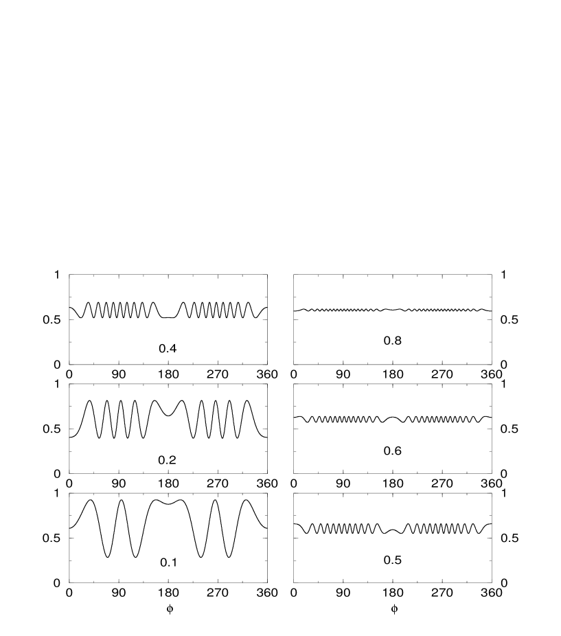
Figure 6 shows that an unabiguous signal would be obtained with about one year’s Borexino statistics for $\Delta m^{2}$ in the range 0.1–0.5. For $\Delta m^{2}=0.6$ there is a signal at $\Delta m_{v}^{2}=0.6$ that might be a little ambiguous with only one year’s statistics, but it retains its shape with increasing statistics; a secondary peak seen at about $\Delta m_{v}^{2}=0.75$ with one year’s statistics goes away with the higher statistics. There is no signal apparent for the $\Delta m^{2}=0.8$ case, as one would expect from looking at the corresponding curve in Figure 4.

Figure 7 shows the extraction of the signal for $\Delta m^{2}$ an order of magnitude lower. Curves correspond to values in Figure 3. Below $\Delta m^{2}=0.04$ this particular analysis starts to become ambiguous. However the slow rate of variation with $\phi$ makes direct comparison with the patterns seen in Figure 3 practical. At $\Delta m^{2}=0.01$ the analysis is complicated by the large change in magnitude of the rate throughout the year with a small increment in the value of $\Delta m^{2}$.

IV Discussion

Based on the SNO result it now seem likely that the solar neutrino puzzle has been solved. It is not a deficiency in the standard solar model that is being observed but new physics. Electron neutrinos are oscillating into some combination of $\mu$ and $\tau$ neutrinos. Exactly how this happens is perhaps not yet clear, whether by one of the MSW solutions or some vacuum mixing solution. In the previous sections of this paper it has been shown that if the solution to the solar neutrino puzzle happens to be maximal mixing in the mass range $\Delta m^{2}=\sim 10^{-10}-6\times 10^{-9}$(eV)², then a proper analysis of a successful ⁷Be neutrino experiment should be able to unambiguously determine $\Delta m^{2}$. Not seeing a $\Delta m^{2}$ signal in this mass range would elimate a region of $\Delta m^{2}$ for large mixing angle.

V Acknowledgments

I would like to thank Chellis Chasman for reading and commenting on the manuscript.

This manuscript has been authored under Contract No. DE-AC02-98CH10886 with the U. S. Department of Energy.

A The day-night effect in the limit of maximal two neutrino mixing

Guth, Randall, and Serna[25] have pointed out that there can be a day-night effect, even for the case of maximal mixing. What follows is a compact explication of this point with emphasis on the limits of no MSW and maximal MSW effect in the sun.

The general form for two mass eigenstates in two neutrino mixing is

$$|\nu_{1}\!>={\rm cos}\theta|\nu_{e}\!>+\ {\rm sin}\theta|\nu_{x}\!>$$ (A1)

and

$$|\nu_{2}\!>=-{\rm sin}\theta|\nu_{e}\!>+\ {\rm cos}\theta|\nu_{x}\!>\ ,$$ (A2)

where $|\nu_{x}\!>$ is presumed to be some linear combination of $|\nu_{\mu}\!>$ and $|\nu_{\tau}\!\!>$. Conversely

$$|\nu_{e}\!>={\rm cos}\theta|\nu_{1}\!>-\ {\rm sin}\theta|\nu_{2}\!>$$ (A3)

and

$$|\nu_{x}\!>={\rm sin}\theta|\nu_{1}\!>+\ {\rm cos}\theta|\nu_{2}\!>\ .$$ (A4)

In free space mass eigenstates propagate independently. A mixed mass state $|\nu(t)\!>$ then has the form

$$|\nu(t)\!>=e^{-im_{1}^{2}t/2E}A_{1}|\nu_{1}\!>+\ e^{-im_{2}^{2}t/2E}A_{2}|\nu_{2}\!>.$$ (A5)

The probability $P_{s}$ that a neutrino born in the sun is an electron neutrino when it reaches the earth is then

$$P_{s}={\rm cos}^{2}\theta P_{1}+{\rm sin}^{2}\theta P_{2}$$ (A6)

with $P_{1,2}=|A_{1,2}|^{2}$ the average probability of a mass one or mass two eigenstate arriving at the earth where the phase has been averaged by the distances involved. Since $P_{1}=1-P_{2}$ this may also be written equivalently

$$P_{2}={({\rm cos}^{2}\theta-P_{s})\over{\rm cos}2\theta}$$ (A7)

The probability $P$ that an electron neutrino born in the sun will be an electron neutino after passing through the sun, traveling to the earth, and then passing through the earth is simply

$$P=P_{2}P_{2e}+(1-P_{2})(1-P_{2e})$$ (A8)

where $P_{2e}$ is the probability that a mass 2 neutrino entering the earth emerges at the detector as an electron neutrino. Making use of Eq.(A7) this becomes

$$P=P_{s}+{(1-2P_{s})\over{\rm cos}2\theta}(P_{2e}-{\rm sin}^{2}\theta).$$ (A9)

This expression is the Mikeyev-Smirnov expression[32] for the day night effect, trivially transformed[26] to be most transparent in various limits.

The maximum value for $P_{s}$ occurs for vacuum oscillations

$$P_{s}=1-{1\over 2}{\rm sin}^{2}2\theta$$ (A10)

and

$${(1-2P_{s})\over{\rm cos}2\theta}=-{\rm cos}2\theta.$$ (A11)

The minimum value for $P_{s}$ occurs for complete adiabatic MSW conversion to a pure mass eigenstate $|\nu_{2}\!>$. In this case from Eq.(A6)

$$P_{s}={\rm sin}^{2}\theta$$ (A12)

and

$${(1-2P_{s})\over{\rm cos}2\theta}=1.$$ (A13)

Thus as $\sin 2\theta$ goes to 1 (maximal mixing) there is no day-night effect for vacuum oscillations and a maximum effect possible in the case of complete adiabatic conversion.

FIG. 1.: Temperature broadening of ⁷Be neutrinos originating in the sun (see text).

FIG. 2.: Top panel: Constant $A$ and oscillating $B$ part of electron neutrino rate emerging from the sun for $\sin^{2}2\theta=1$ (solid line) and for $\sin^{2}2\theta=0.9$, (dotted line); Bottom panel: Total oscillation damping factor (solid line) and partial damping factors (see text).

FIG. 3.: Rate of ⁷Be neutrinos detected by electron scattering for maximal mixing. The number on each panel gives $\Delta m^{2}$ for the solid line. The long and short dashed line is $\Delta m^{2}$ plus approximately 0.00035, the short dashed line $\Delta m^{2}$ plus 0.0007, the long dashed line $\Delta m^{2}$ plus 0.00105 and the dotted line $\Delta m^{2}$ plus 0.0014.

FIG. 4.: Rate of ⁷Be neutrinos detected by electron scattering for maximal mixing. The number on each panel gives $\Delta m^{2}$ for the solid line.

FIG. 5.: The top panel gives the rate of ⁷Be neutrinos coming from the sun for maximal mixing and $\Delta m^{2}$ = 0.3. The solid line in the middle panel gives the absolute value of the Fourier analysis of the distribution $|I(0.5,\Delta m_{v}^{2})|$ and the dashed line the absolute value of the analysis of the constant average of the distribution $|J(\Delta m_{v}^{2})|$. The bottom panel shows the absolute value of the difference of the Fourier analyses of the distribution and the constant average of the distribution $|K(0.5,\Delta m_{v}^{2})|$. This is the quantity that extracts the $\Delta m^{2}$ signal.

FIG. 6.: Extraction of the the signal $|K(\Delta m^{2},\Delta m_{v}^{2})|$. The number on each panel gives the value of $\Delta m^{2}$. The dotted line lines represents 15000 tries or about 9000 events. The solid lines represent four times the statistics: 60000 tries or about 36000 events.

FIG. 7.: $|K(\Delta m^{2},\Delta m_{v}^{2})|$ as in Figure 6, but for lower values of $\Delta m^{2}$. The location of the peak becomes less well defined with decreasing $\Delta m^{2}$. As in Figure 3 the long and short dashed line is $\Delta m^{2}$ plus approximately 0.00035, the short dashed line $\Delta m^{2}$ plus 0.0007, the long dashed line $\Delta m^{2}$ plus 0.00105 and the dotted line $\Delta m^{2}$ plus 0.0014.

REFERENCES

- [1] Anthony J. Baltz, Alfred Scharff Goldhaber, and Maurice Goldhaber, Phys. Rev. Lett. 81, 5730 (1998).
- [2] J. N. Bahcall and R. N. Ulrich, Rev. Mod. Phys. 60, 297 (1988).
- [3] J. N. Bahcall and M. H. Pinsonneault, Rev. Mod. Phys. 64, 885 (1992).
- [4] John N. Bahcall, M. Pinsonneault, and G. J. Wasserburg, Rev. Mod. Phys. 67, 781 (1995).
- [5] J. N. Bahcall, S. Basu, and M. H. Pinsonneault, Phys. Lett. B 433, 1 (1998)
- [6] J. N. Bahcall, P. I. Krastev, and A. Yu. Smirnov, Phys. Rev. D 58, 096016 (1998).
- [7] Y. Fukuda et al. (Super-Kamiokande Collaboration), Phys. Rev. Lett. 81, 1158 (1998).
- [8] Q. R. Ahmed, et al. (SNO Collaboration), Phys. Rev. Lett. 87, 071301 (2001)
- [9] B. T. Cleveland et al., Astrophys. J. 496, 505 (1998).
- [10] W. Hampel et al. (GALLEX Collaboration), Phys. Lett. B 447, 127 (1999).
- [11] J. N. Abdurashitov et al. (SAGE Collaboration), Phys. Rev. C 60, 055801 (1999).
- [12] John N. Bahcall, M. C. Gonzalez-Garcia, and Carlos Peña-Garay, arXiv:hep-ph/0106258.
- [13] G. L. Fogli, E. Lisi, D. Mantanino, and A. Palazzo, arXiv:hep-ph/0106247.
- [14] N. Hata, and P. G. Langacker, Phys. Rev. D 56, 6107 (1997).
- [15] James M. Gelb and S. P. Rosen, Phys. Rev. D 60, 011301 (1999).
- [16] P. I. Krastev and S. T. Petcov, Nucl. Phys. B 449, 605 (1995).
- [17] James M. Gelb and S. P. Rosen, arXiv:hep-ph/9908325.
- [18] André de Gouvêa, Alexander Friedland, and Hitoshi Murayama, Phys. Rev. D 60, 093011 (1999).
- [19] Borexino Collaboration, G. Alimonti et al., arXiv:hep-ex/0012030.
- [20] M. Cribier for the LENS collaboration, Nucl. Phys. B (Proc. Suppl.)87, 195, (2000).
- [21] P. Gorodetzky, A. de Bellefon, J. Dolbeau, T. Patzak, P. Salin, A. Sarrat, J. C. Vanel, Nucl. Phys. B (Proc. Suppl.)87, 506, (2000).
- [22] J. N. Bahcall, Neutrino Astophysics, Cambridge University Press (1989).
- [23] Sandip Pakvasa and James Pantaleone, Phys. Rev. Lett. 65, 2479 (1990).
- [24] John N. Bahcall, Phys. Rev. D 49, 3923 (1994).
- [25] Alan H. Guth, Lisa Randall, and Mario Serna, JHEP 9908, 018 (1999).
- [26] A. J. Baltz and J. Weneser, Phys. Rev. D 50 5971 (1994).
- [27] J. Pantaleone, Phys. Lett. B 251, 618 (1990).
- [28] A. J. Baltz and J. Weneser, Phys. Rev. D 35 528 (1987); D 37 3364 (1988); E. D Carlson, Phys. Rev. D 34, 1454 (1986); J. Bouchez, M. Cribier, W. Hampel, J. Rich, M. Spiro, and D. Vignaud, Z. Phys. C 32, 499 (1986).
- [29] R. S. Raghavan, A. B. Balantekin, F. Loreti, A. J. Baltz, S. Pakvasa, and J. Pantaleone, Phys. Rev. D 44, 3786 (1991).
- [30] A. De Rujula and S. Glashow, CERN-TH 6655/92 (1992).
- [31] G. L. Fogli, E. Lisi and D. Mantanino, Phys. Rev. D 56 4374 (1997).
- [32] S. P. Mikheyev and A. Yu. Smirnov, in New and Exotic Phenomena, Proceedings of the Moriond Workshop, Les Arc, Savoie, France, 1987, edited by O. Fackler and J. Tran Thanh Van (Editions Frontiìeres, Gif-sur-Yvette, France, 1987), p. 405.