SLAC-PUB-8863 June 2001

Probes Of Universal Extra Dimensions at Colliders

Thomas G. Rizzo Stanford Linear Accelerator Center

Stanford University

Stanford CA 94309, USA

In the Universal Extra Dimensions model of Appelquist, Cheng and Dobrescu, all of the Standard Model fields are placed in the bulk and thus have Kaluza-Klein(KK) excitations. These KK states can only be pair produced at colliders due to the tree-level conservation of KK number, with the lightest of them being stable and possibly having a mass as low as $\simeq 350-400$ GeV. After calculating the contribution to $g-2$ in this model we investigate the production cross sections and signatures for these particles at both hadron and lepton colliders. We demonstrate that these signatures critically depend upon whether the lightest KK states remain stable or are allowed to decay by any of a number of new physics mechanisms. These mechanisms which induce KK decays are studied in detail.

1 Introduction

The possibility that the gauge bosons of the Standard Model(SM) may be sensitive to the existence of extra dimensions near the TeV scale has been known for some time[1]. However, one finds that the phenomenology of these models is particularly sensitive to the manner in which the SM fermions (and Higgs bosons) are treated.

In the simplest scenario, the fermions remain on the wall located at the fixed point $y_{i}=0$ and are not free to experience the extra dimensions. (Here, lower-case Roman indices label the co-ordinates of the additional dimensions while Greek indices label our usual 4-d space-time.) However, since 5-d translational invariance is broken by the wall, the SM fermions interact with the Kaluza-Klein(KK) tower excitations of the SM gauge fields in the usual trilinear manner, i.e., $\sim gC_{n}\bar{f}\gamma_{\mu}fG^{\mu}_{(n)}$, with the $C_{n}$ being some geometric factor and $n$ labelling the KK tower state with which the fermion is interacting. Current low-energy constraints arising from, e.g., $Z$-pole data, the $W$ boson mass and $\mu$-decay generally require the mass of the lightest KK gauge boson to be rather heavy, $\mathrel{\mathchoice{\lower 3.01385pt\vbox{\halign{$\matth\displaystyle\hfil#\hfil$\cr>\crcr\sim\crcr}}}{\lower 3.01385pt\vbox{\halign{$\matth\textstyle\hfil#\hfil$\cr>\crcr\sim\crcr}}}{\lower 3.01385pt\vbox{\halign{$\matth\scriptstyle\hfil#\hfil$\cr>\crcr\sim\crcr}}}{\lower 3.01385pt\vbox{\halign{$\matth\scriptscriptstyle\hfil#\hfil$\cr>\crcr\sim\crcr}}}}4$ TeV in the case of the 5-d SM[2] independent of whether or not the Higgs fields are on the wall under the assumption that the $C_{n}$ are $n$-independent for $n\geq 1$.

A second possibility occurs when the SM fermions experience extra dimensions by being ‘stuck’, i.e., localized or trapped at different specific points in a thick brane[3] away from the conventional fixed points. It has been shown that such a scenario can explain the absence of a number of rare processes, such as proton decay, by geometrically suppressing the size of the Yukawa couplings associated with the relevant higher dimensional operators without resorting to the existence of additional symmetries of any kind. In addition such a scenario may be able to explain the fermion mass hierarchy and the observed CKM mixing structure thus addressing important issues in flavor physics[4]. The couplings of the SM fermions to the gauge KK towers are in this case dependent upon their location in the extra dimension(s).

A last possibility, perhaps the most democratic, requires all of the SM fields to propagate in the $\sim$ TeV^-1 bulk[5], i.e., Universal Extra Dimensions(UED). In this case, there being no matter on the walls, the conservation of momentum in the extra dimensions is restored and one now obtains interactions in the 4-d Lagrangian of the form $\sim gC_{ijk}\bar{f}^{(i)}\gamma_{\mu}f^{(j)}G^{\mu}_{(k)}$, which for flat space metrics vanishes unless $i+j+k=0$, as a result of the afore mentioned momentum conservation. Although this momentum conservation is actually broken by orbifolding, one finds, at tree level, that KK number remains a conserved quantity. (As we will discuss below this conservation law is itself further broken at one loop order.) This implies that pairs of zero-mode fermions, which we identify with those of the SM, cannot directly interact singly with any of the excited modes in the gauge boson KK towers. Such a situation clearly limits any constraints arising from precision measurements since zero mode fermion fields can only interact with pairs of tower gauge boson fields. In addition, at colliders it now follows that KK states must be pair produced, thus significantly reducing the possible direct search reaches for these states. In fact, employing constraints from current experimental data, Appelquist, Cheng and Dobrescu(ACD)[5] find that the KK states in this scenario can be as light as $\simeq 350-400$ GeV, much closer to current energies than the KK modes in the first case discussed above. If these states are, in fact, nearby, they will be copiously produced at the LHC, and possibly also at the Tevatron, in a variety of different channels. It is the purpose of this paper to estimate the production rates for pairs of these particles in various channels and to discuss their possible production signatures. This is made somewhat difficult by the apparent conservation of KK number which appears to forbid the decay of heavier excitations into lighter ones and is a point we will return to in detail below.

The outline of this paper is as follows: in Section II we briefly discuss the particle spectrum in the UED model and the breaking of KK number to ‘KK parity’ at one loop. In Section III, in an attempt to get a further handle on the compactification scale of the UED scenario, we discuss the shift in the value of $g-2$ predicted in this model. Unfortunately, as we will see, no new constraints are obtained. In Section IV we discuss the production mechanisms and cross sections for pairs of KK excitations of the SM fields at the Tevatron and LHC. Similar production mechanisms and $e^{+}e^{-}$ and $\gamma\gamma$ colliders are also briefly considered. Section V discusses the possible signatures for KK pair production addressing the issue of their possible stability in light of our earlier discussions in Section II. Three particular decay scenarios are considered. A discussion and our conclusions can be found in Section VI.

2 Model Set-up Review

In this section we very briefly review the basic nature of the UED model. The essential idea is that all of the fields of the SM are put in the bulk and thus have KK excitations. For simplicity in what follows we will limit our discussion to the case of one extra dimension with the extension to more than one dimension being reasonably straightforward. Due to $S_{1}/Z_{2}$ orbifolding, which is necessary to obtain chiral zero mode fermions, the fields can be classified as either $Z_{2}$ even or odd: all Higgs boson and 4-d gauge fields are taken as $Z_{2}$ even whereas the 5-d components of the gauge fields (which are not present in the Unitary Gauge) must then be $Z_{2}$ odd. Taking the compactification radius to be $R=1/M_{c}$ the corresponding eigenfunctions are simply $\sim\cos~{}ny/R~{}(\sin~{}ny/R)$ for the $Z_{2}$ even(odd) fields. The gluon and photon excitations have the usual KK masses, $nM_{c}$, while the $W$ and $Z$ towers have shifted masses $[M_{W,Z}^{2}+(nM_{c})^{2}]^{1/2}$ after spontaneous symmetry breaking(SSB) by the zero mode Higgs field. Although the zero mode Goldstone bosons are eaten as part of the SSB mechanism, their tower states remain physical, level by level degenerate with the gauge bosons and are also $Z_{2}$ even. In the fermion sector there is a well-known doubling of states; every $SU(2)_{L}$ doublet $D$ or singlet $S$ field has a vector-like tower of states above the chiral zero mode. $S_{1}/Z_{2}$ only allows for the existence of the left-handed (right-handed) zero mode for the $D$($S$). Note that while one of the fermion KK towers, the one matching the chirality of the zero mode, is constrained to be $Z_{2}$ even, the other must be $Z_{2}$ odd.) Note that in performing calculations one must be careful not to confuse the $S_{L}$ and $D_{L}$ fields and their corresponding right-handed partners. As will be discussed below, the zero mode Higgs vev links the $S$ and $D$ states level by level and simultaneously generates the zero mode fermion masses as usual. The Yukawa coupling of this interaction is completely fixed by the SM fermion mass. This cross linking of the the two towers $D$ and $S$ will be necessary in order to generate the $g-2$ of the muon in this model.

Now although the KK number is conserved at the tree level it becomes apparent that it is no longer so at loop order[6]. Consider a self-energy diagram with a field that has KK number of $2n(2n+1)$ entering and a zero($n=1$) mode leaving the graph; KK number conservation clearly does not forbid such an amplitude and constrains the 2 particles in the intermediate state to both have KK number $n$($n$ and $n+1$). The existence of such amplitudes implies that all even and odd KK states mix separately so that the even KK excitations can clearly decay to zero modes while odd KK states can now decay down to the KK number=1 state. Thus it is KK parity, $(-1)^{n}$, which remains conserved while KK number itself is broken at one loop. Since the lightest KK excited states with $n=1$ have odd KK parity they remain stable unless new physics is introduced. As we are only concerned with the production of pairs of the lightest KK particles in our discussion below, we are faced with the possibility of producing heavy stable states at colliders. This point will be discussed in detail further below.

3 $g-2$

The bound on $M_{c}$ obtained by ACD in this model is quite low and is not improved by the consideration of other processes such as $b\rightarrow s\gamma$ as discussed by Agashe, Deshpande and Wu[7]. To see if we can improve this bound on $M_{c}$, we briefly discuss the contribution to $g-2$ in the UED model; we follow the analysis as given in[8, 9]. To this end we consider the specific situation where we have two fermions in the bulk, $D_{\mu}$ and $S_{\mu}$, corresponding to the 5-dimensional muon fields, having the quantum numbers of an $SU(2)_{L}$ doublet and singlet with weak hypercharges $Y=-1/2$ and $-1$, respectively. (We will drop the $\mu$ index on these fields in what follows as it is clearly understood what fields we are discussing.) The interactions of these fermions with the gauge fields can be described by the action,

$$S_{fV}=\int d^{4}x\int dy\left[V^{M}_{n}\left({i\over{2}}\overline{S}\,\gamma^{n}\,{\cal D}_{M}S+h.c.\right)-sgn(y)m_{S}\overline{S}S+(S\rightarrow D\right)],$$ (1)

where, $V$ is the vielbein, which is trivial for the flat space case we are considering, ${\cal D}_{M}$ is a covariant derivative and $h.c.$ denotes the Hermitian conjugate term. Note that gauge interactions do not mix the $D$ and $S$ fields. The $D$ and $S$ fields also interact with the bulk Higgs isodoublet field, $H^{0}$, i.e.,

$$S_{fH}={(2\pi R)^{1/2}\lambda}\int d^{4}x\int dy\ \overline{S}DH^{0}\ +h.c.,$$ (2)

with $R$ being the compactification radius as described above and $\lambda$ being a dimensionless Yukawa coupling. Due to the KK mechanism the fields $D_{L,R}^{(n)}$ and $S_{L,R}^{(n)}$ form separate 4-d towers of Dirac fermions which, as discussed above, are degenerate level by level. These KK expansions can be written as $D=\sum D_{L}^{(n)}(x)\chi^{(n)}(y)+D_{R}^{(n)}(x)\tau^{(n)}(y)$ and $S=\sum S_{L}^{(n)}(x)\tau^{(n)}(y)+S_{R}^{(n)}(x)\chi^{(n)}(y)$ where the $\chi(\tau)$ fields are $Z_{2}$ even(odd). Note that the $Z_{2}$ orbifold symmetry and orthonormality only allows ‘level-diagonal’ couplings of both types: $\overline{D_{L}}^{(n)}S_{R}^{(n)}+h.c.$ and $\overline{D_{R}}^{(n)}S_{L}^{(n)}+h.c.$. The value of $\lambda$ is fixed by requiring the zero mode fermion obtain a mass $m_{\mu}$ after the Higgs zero mode obtains a vev, $v$, and tells us the level by level coupling between the tower members.

In terms of the $D$ and $S$ fields, the operator which generates the anomalous magnetic dipole moment of the $\mu$ can be written as $D_{L}^{(0)}\sigma_{\mu\nu}q^{\nu}S_{R}^{(0)}+h.c.$. This reminds us that this operator and the muon mass generating term have the same isospin and helicity structure such that a Higgs interaction is required in the form of a mass insertion to connect the two otherwise decoupled zero modes. We can think of this mass insertion as the interaction of a fermion with an external Higgs field that has been replaced by its vev.

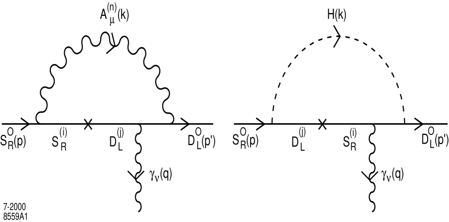
Figure 1: Typical Feynman diagrams for the gauge and Higgs boson contribution to $(g-2)_{\mu}$. The mass insertion is denoted by the cross.

Helicity flips play an important role in evaluating the contributions to $(g-2)_{\mu}$ since muon KK excitations are now propagating inside the loop. As is well-known, for non-chiral couplings the contribution to the anomalous magnetic moment of a light fermion can be enhanced when a heavy fermion of mass $m_{h}$ participates inside the loop[10]. There are a number of diagrams that can contribute to $(g-2)_{\mu}$ at one loop of which two are shown in Fig. 1. The diagram on the left corresponds to the exchange of a tower of the 4-d neutral gauge bosons, $\gamma^{(n)}$ and/or $Z^{(n)}$, which we will now discuss in detail. Due to gauge invariance we are free to choose a particular gauge in order to simplify the calculation. Here, we make use of the $\xi=1$ unitary gauge where the numerator of the 4-d propagator is just the negative of the flat space metric tensor[11]. Hence, in this gauge, the loops with the 4-d components of the gauge fields and the ones with the fifth component need to be considered separately. In this example, the mass insertion takes place inside the loop before the photon is emitted. Clearly there are three other diagrams of this class: two with the mass insertion on an external leg and the third with the mass insertion inside the loop but after the photon is emitted. The amplitude arising from this vector exchange graph is given by

$${\cal M}_{V} = g_{L}g_{R}~{}\bar{u}(p^{\prime})\ (ie\gamma_{\mu})P_{L}~{}i{{\hat{\not\!p^{\prime}}+m_{n}}\over{\hat{p}^{\prime 2}-m_{n}^{2}}}\ (-ie\gamma_{\nu})P_{L}\,$$ (3)

$$\times i{{\hat{\not\!p}+m_{n}}\over{\hat{p}^{2}-m_{n}^{2}}}\ (im_{\mu}P_{R})\ ~{}i{{\hat{\not\!p}+m_{n}}\over{\hat{p}^{2}-m_{n}^{2}}}\ (ie\gamma^{\mu})P_{R}\ u(p)\ {-i\over{k^{2}-m_{A}^{(n)~{}2}}}+h.c.\,,$$

where $g_{L,R}$ are the corresponding couplings of the SM gauge boson to the $\mu$ in units of $e$ and $\hat{p}(\hat{p}^{\prime})=p(p^{\prime})-k$. Here (in the limit that we can neglect the muon mass) $m_{n}=nM_{c}$ are the masses of the $D$ or $S$ muonic KK states and $m_{A}^{(n)}$ are the corresponding masses of the KK gauge tower states, $[m_{A}^{(0)2}+(nM_{c})^{2}]^{1/2}$, with $M_{c}$ being the compactification scale. Note that the mass insertion, $m_{\mu}$, comes with a chirality factor that can be determined from the action $S_{fH}$. The amplitude where the mass insertion comes after the photon emission can be easily obtained by interchanging the ordering in the resulting final amplitude expression.

What happens when the mass insertion occurs on the external legs? With some algebra it is straightforward to show that the corresponding amplitudes obtained in these two cases are suppressed in comparison to the case of internal insertion by at least a factor of order $\sim m_{\mu}/M_{KK}$, where $M_{KK}$ is a typical large KK mass. In the case of the $W$ gauge boson tower graphs, since the $W$ couples only to the $D$’s, the mass insertion must occur on the incoming leg of the graph and the photon is then emitted from the $W$; this graph can also be shown to produce a sub-leading contribution by at least a factor of order $\sim m_{\mu}/M_{KK}$. Thus, $W$ tower graphs can be safely ignored in comparison to those arising from the $Z$ and $\gamma$ towers. (Note that the suppressions that we obtain here in the case of heavy internal KK states are absent in the SM calculation of $g-2$ since the muon or its neutrino are now the internal loop fermion). In a similar fashion it is clear that the graphs containing Goldstone bosons will also be suppressed since their couplings are of order $m_{\mu}/M_{W}$.

The next class of graphs is similar to the 4-d vector exchange, but in the $\xi=1$ gauge, now involves the fifth component of the original 5-d field. Here it is important to recall that these fifth components are $Z_{2}$ odd fields thus connecting $S_{L}(D_{L})$ with $S_{R}(D_{R})$. Let us first consider the case where the neutral 4-d vector field is replaced by the 5-d scalar field; in analogy with Fig.1 we obtain:

$${\cal M}_{5} = g_{L}g_{R}~{}\bar{u}(p^{\prime})\ ieP_{R}~{}i{{\hat{\not\!p^{\prime}}+m_{n}}\over{\hat{p}^{\prime 2}-m_{n}^{2}}}\ (-ie\gamma_{\nu})P_{R}\,$$ (4)

$$\times i{{\hat{\not\!p}+m_{n}}\over{\hat{p}^{2}-m_{n}^{2}}}\ (im_{\mu}P_{L})\ ~{}i{{\hat{\not\!p}+m_{n}}\over{\hat{p}^{2}-m_{n}^{2}}}\ ieP_{R}\ u(p)\ {1\over{k^{2}-m_{A}^{(n)~{}2}}}+h.c.\,,$$

As before, the amplitude where the mass insertion comes after the photon emission can be easily obtained by interchanging the ordering in the resulting final amplitude expression. Also, as before, a short analysis shows that graphs with external insertions or those involving a $W_{5}$ or a Higgs field lead to terms which are subleading in $m_{\mu}/M_{KK}$ or $m_{\mu}/M_{W}$. We thus obtain the total contribution to $g-2$ from a given KK level of a neutral gauge boson by adding the two expressions above and performing the momentum integrations; we find

$$(g-2)_{n}={-3e^{2}g_{L}g_{R}m_{\mu}^{2}\over{16\pi^{2}m_{n}^{2}}}\int^{1}_{0}dx\int^{1-x}_{0}dy{6x^{2}+12xy-11x\over{1+\epsilon_{n}(x+y)}}\,,$$ (5)

where we have defined $m_{A}^{(n)2}=m_{n}^{2}(1+\epsilon_{n})$; note that $\epsilon_{n}=0$ in the case of photons. To go further we must sum over both the the photon and Z towers; using $\sum_{1}^{\infty}{1\over{n^{2}}}={\pi^{2}\over{6}}$ and $\sum_{1}^{\infty}{1\over{n^{4}}}={\pi^{4}\over{90}}$ we obtain the final numerical result

$$(g-2)_{UED}=-439\cdot 10^{-11}(M_{Z}^{2}/M_{c}^{2})[1-0.23(M_{Z}^{2}/M_{c}^{2})+...]\,$$ (6)

where we have neglected higher order terms in the ratio $M_{Z}^{2}/M_{c}^{2}$. For $M_{c}=300$ GeV, the smallest possible value, this gives $(g-2)_{UED}\simeq-40\cdot 10^{-11}$ which is only one quarter as large as the SM electroweak contribution. This is too small to make much of an impact on the potential difference between the experimental data and the SM prediction[12, 13]. Thus we conclude that $g-2$ does not yet provide any useful constraint on the UED scenario[14].

4 Collider Production

Due to the conservation of KK number at tree-level, KK excitations of the SM fields must be pair-produced at colliders. At $\gamma\gamma$ and lepton colliders the production cross sections for all the kinematically accessible KK states will very roughly be of order 100 fb $(1~{}TeV/\sqrt{s})^{2}$ which yields respectable event rates for luminosities in the $100-500~{}fb^{-1}$ range. A sample of relevant cross sections at both $\gamma\gamma$ and $e^{+}e^{-}$ colliders are shown in Fig. 2. In the case of $\gamma\gamma$ collisions we have chosen the process $\gamma\gamma\rightarrow W^{+(1)}W^{-(1)}$ as it the process which has the largest cross section for the production of the first KK state. Similarly, gauge boson pair production in $e^{+}e^{-}$ collisions naturally leads to a large cross section. Clearly, such states once produced would not be easily missed for masses up to close the kinematic limit of the machine independently of how they decayed or if they were stable. To directly probe heavier masses we must turn to hadron colliders.

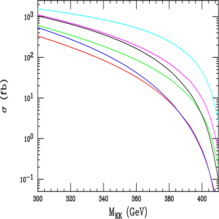
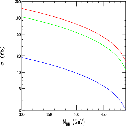
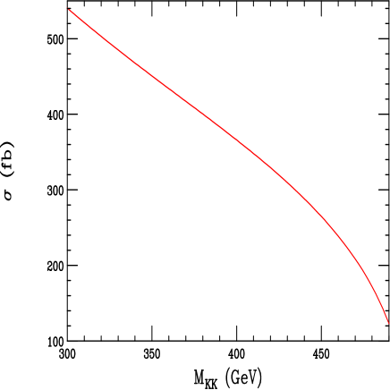
Figure 2: Cross section for $\gamma\gamma\rightarrow W^{(1)+}W^{(1)-}$ (top panel) for different electron and laser polarizations for $\sqrt{s}_{ee}=1$ TeV. Cross section for $e^{+}e^{-}\rightarrow W^{(1)}W^{(1)}$ (lower right panel) for $\sqrt{s}=1$ TeV. Cross sections for (top to bottom, lower left panel) $e^{+}e^{-}\rightarrow 2\gamma^{(1)}$, $Z^{(1)}\gamma^{(1)}$ and $2Z^{(1)}$ for $\sqrt{s}=1$ TeV.

Since both QCD and electroweak exchanges can lead to KK pair production at hadron colliders there are three classes of basic processes to consider. Clearly the states with color quantum numbers will have the largest cross sections at hadron machines and there are a number of processes which can contribute to their production at order $\alpha_{s}^{2}$[15] several of which we list below:

$$(i)~{}~{}gg \rightarrow g^{(1)}g^{(1)}\,$$

$$(ii)~{}~{}qq^{\prime} \rightarrow q^{(1)}q^{\prime(1)}\,$$

$$(iii)~{}~{}gg+q\bar{q} \rightarrow q^{\prime(1)}\bar{q}^{\prime(1)}\,$$

$$(iv)~{}~{}qq \rightarrow q^{(1)}q^{(1)}\,$$

$$(v)~{}~{}q\bar{q} \rightarrow q^{(1)}q^{(1)}\,,$$ (7)

where the primes are present to denote flavor differences. Fig. 3 shows the cross sections for these five processes at both the $\sqrt{s}=2$ TeV Tevatron and the LHC summed over flavors. It is clear that the during the Tevatron Run II we should expect a reasonable yield of these KK particles for masses below $\simeq 600$ GeV if integrated luminosities in the range of 10-20 $fb^{-1}$ are obtained. Other processes that we have not considered may be able to slightly increase this reach. For larger masses we must turn to the LHC where we see that significant event rates should be obtainable for KK masses up to $\simeq 3$ TeV or so for an integrated luminosity of 100 $fb^{-1}$. As one might expect we see that the most important QCD processes for the production of KK states are different at the two colliders.

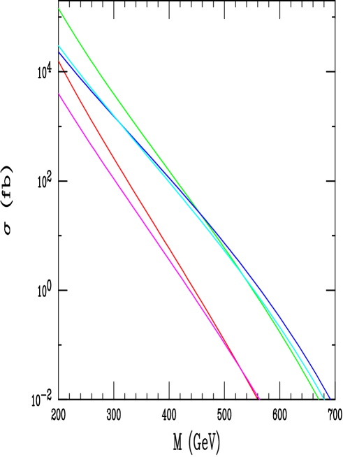
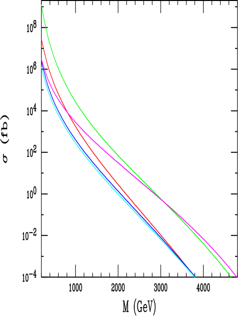
Figure 3: Cross section for the pair production of the lightest colored KK states at the $\sqrt{s}=2$ TeV Tevatron(top) and the LHC(bottom). In the top panel, from top to bottom on the left-hand side, the curves correspond to the processes $ii,v,iii,i$ and $iv$, respectively. In the bottom panel, from top to bottom on the left-hand side, the curves correspond to the processes $ii,i,iv,iii$ and $v$, respectively. Antiquark contributions are included in reactions $ii$ and $iv$.

The real signature of the UED scenario is that all of the SM fields have KK excitations. Thus we will also want to observe the production of the SM color singlet states. Of course color singlet states can also be produced with the largest cross sections being for associated production with a colored state at order $\alpha\alpha_{s}$; these rates are of course smaller than for pairs of colored particles as can be seen in Fig. 4. Here we see reasonable rates are obtained for KK masses in excess of $\simeq 1.8$ TeV or so.

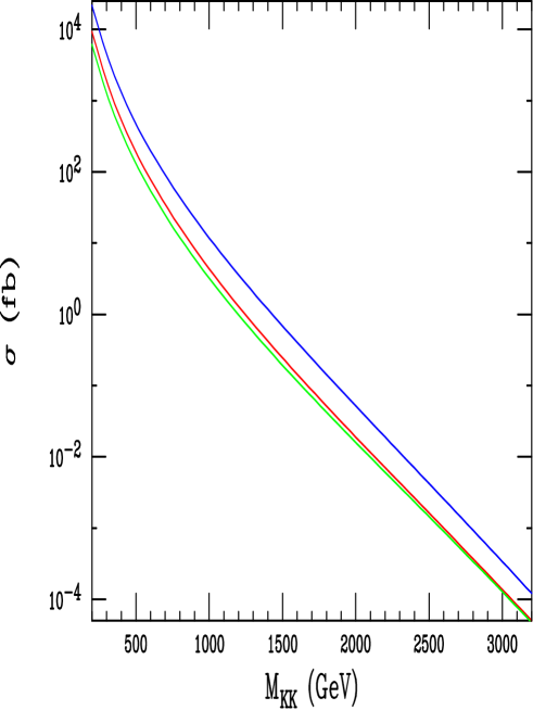
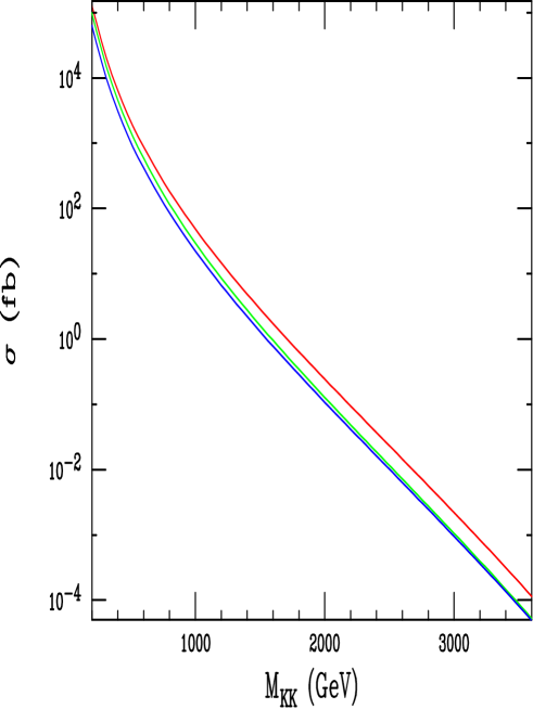
Figure 4: Cross sections for the associated production of the lightest color singlet KK states at the LHC: in the top panel, from top to bottom, for $g^{(1)}W^{(1)\pm},g^{(1)}Z^{(1)}$ and $g^{(1)}\gamma^{(1)}$ final states; in the lower panel, from top to bottom, for $q^{(1)}W^{(1)\pm},q^{(1)}Z^{(1)}$ and $q^{(1)}\gamma^{(1)}$ final states. Anti-quark and contributions are included.

Lastly, it is possible to pair produce color singlets via electroweak interactions which thus lead to cross sections of order $\alpha^{2}$. Due to the large center of mass energy of the LHC these cross sections can also lead to respectable production rates for KK masses as great as $\simeq 1.5$ TeV as can be seen from Fig. 5.

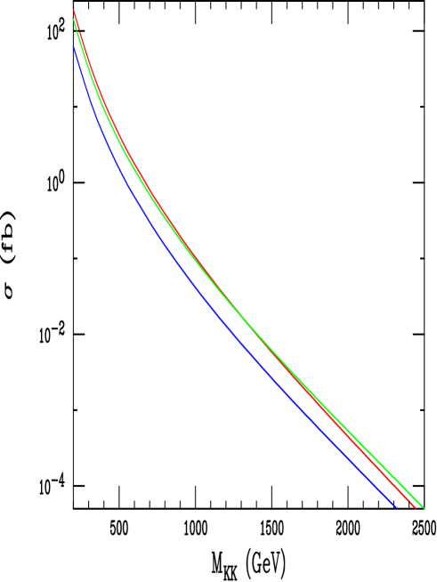
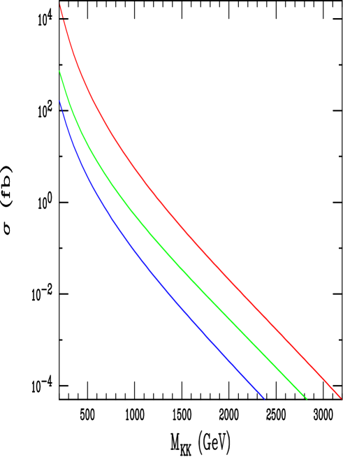
Figure 5: Cross sections for the production of the lightest color singlet KK states at the LHC: in the top panel, from top to bottom, for $2Z^{1)},\gamma^{(1)}Z^{(1)}$ and $2\gamma^{(1)}$ final states; in the bottom panel, from top to bottom, for $W^{(1)+}W^{(1)-},W^{(1)\pm}Z^{(1)}$ and $W^{(1)\pm}\gamma^{(1)}$ final states.

It is clear from this analysis that the LHC will have a significant search reach for both colored and non-colored KK states provided that the production signatures are reasonably distinct. This is the subject for the next section.

5 Collider Signatures

When examining collider signatures for KK pair production in the UED there are two important questions to ask: ($i$) Are the lightest KK modes stable and ($ii$) if they are unstable what are their decay modes? From the discussion above it is clear that without introducing any new physics the $n=1$ KK states are stable so we must consider this possibility when looking at production signatures.

In their paper ACD[5] argue that cosmological constraints possibly suggest that KK states in the TeV mass range must be unstable on cosmological time scales. (Of course this does not mean that they would appear unstable on the time scale of a collider experiment in which case our discussion is the same as that above.) This would require the introduction of new physics beyond that contained in the original UED model. There are several possible scenarios for such new physics. Here we will discuss three possibilities in what follows, the first two of which were briefly mentioned by ACD[5].

Scenario I: The TeV^-1-scale UED model is embedded inside a thick brane in a higher $(\delta+4)$-dimensional space, with a compactification scale $R_{G}>>R_{c}$, in which gravity is allowed to propagate in a manner similar to the model of Arkani-Hamed, Dimopoulos and Dvali[16]. Since the graviton wave functions are normalized on a torus of volume $(2\pi R_{G})^{\delta}$ while the KK states are normalized over $2\pi R_{c}$ the overlap of a KK zero mode with any even or odd KK tower state $n$ and a graviton will be non-zero. In a sense, the brane develops a transition form-factor analogous to that described in [17]. This induces transitions of the form $KK(n=1)\rightarrow KK(n=0)+G$ where $G$ represents the graviton field and appears as missing energy in the collider detector. This means that production of a pair of KK excitations of, e.g., quarks or gluons would appear as two jets plus missing energy in the detector; the corresponding production of a KK excited pair of gauge bosons would appear as the pair production of the corresponding zero modes together with missing energy. We can express this form-factor simply as

$${\cal F}={\sqrt{2}\over{\pi R_{c}}}\int_{0}^{\pi R_{c}}dye^{im_{g}y}(\cos ny/R_{c},\sin ny/R_{c})\,,$$ (8)

for even and odd KK states, respectively, where $m_{g}$ is the graviton mass. Here we have assumed that the thick brane resides at $y_{i}=0$ for all $i\neq 1$. These integrals can be performed directly and we obtain the following expressions for the transition form-factors in the case where $n=1$:

$${\cal F}^{2}_{even}(n=1)={4\over{\pi^{2}}}~{}{x^{2}\over{(1-x^{2})^{2}}}~{}(1-\cos(\pi x))\,,$$ (9)

with ${\cal F}^{2}_{odd}(n=1)={\cal F}^{2}_{even}(n=1)/x^{2}$ where $x=m_{g}R_{c}$. Given these form-factors we can calculate the actual decay rate for $KK(n=1)\rightarrow KK(n=0)+G$, where we now must sum up the graviton towers by following the analyses in Ref.[18]; this result should be relatively independent of the spin of the original KK state. We find the total with to be given by

$$\Gamma={(2\pi)^{\delta/2}~{}\overline{M}_{Pl}^{2}\over{\Gamma(\delta/2)~{}M_{D}^{2+\delta}}}\int^{M_{KK}}_{R_{G}^{-1}}dm_{g}~{}m_{g}^{\delta-1}~{}\Gamma(m_{g})~{}[{\cal F}(m_{g}R_{c})]^{2}(n=1)\,,$$ (10)

where $\Gamma(m_{g})$ is the width for the decay into a graviton of mass $m_{g}$, $M_{D}$ is the $\delta+4$-dimensional Planck scale, $\overline{M}_{Pl}$ is the conventional 4-d reduced Planck scale, and $M_{KK}$ is the mass of the relevant decaying KK state. Performing the integration numerically we obtain the results shown in Fig.6. This figure shows that this mechanism provides for a very rapid decay over almost all of the parameter space. For light KK states with both $\delta$ and $M_{D}$ large the decay rate is suppressed and may lead to finite length charged tracks in the detector. (In particular the production of a charged KK state with a long lifetime would yield a kink-like track structure due to the decay to the graviton tower.) Although not a true two-body decay, Fig.6 also shows that the typical missing energy in the gravitational decay of a KK state will be close to half its mass, which is quite significant for such heavy objects. It is clear that events with such a large fraction of missing energy should be observable above background given sufficient event rates. These events will not be confused with SUSY signals since they occur in every possible channel.

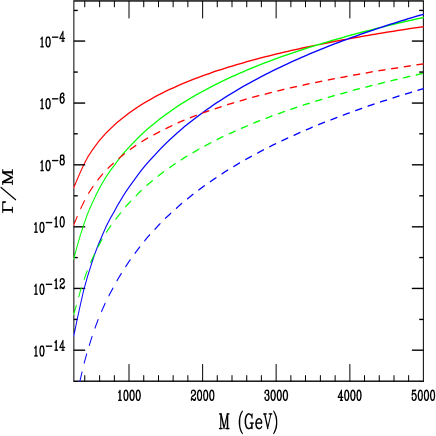
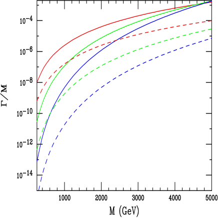
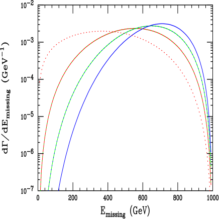
Figure 6: Width for the decay of the first excited KK state (even-top left panel, odd-top right panel) into the corresponding zero mode and a graviton tower as a function of the mass of the KK state. The solid(dashed) lines are for $M_{D}=5(10)$ TeV and from top to bottom in each case the curves correspond to $\delta=2,4,6$, respectively. The lower panel shows the missing energy distribution for these decays for these same cases assuming a KK mass of 1 TeV.

Scenario II: KK decays can be induced in the UED model by adding a ‘benign’ brane at some $y=y_{0}$ which induces new interactions. By ‘benign’ we mean that these new interactions only do what we need them to do and do not alter the basic properties of the UED model. The simplest form of such interactions are just the four dimensional variants of the terms in the the 5-d UED action. For example, one might add a term such as

$$\int d^{4}x\int dy~{}\delta(y-y_{0})~{}{\lambda\over{M_{s}}}\bar{\psi}\gamma^{A}{\cal D}_{A}\psi\,,$$ (11)

where $\lambda$ is some Yukawa-like coupling and $M_{s}$ is some large scale. Note that the brane is placed at some arbitrary position $y=y_{0}$ and not at the fixed points where only even KK modes would be effected. These new interactions result in a mixing of all KK states both even and odd and, in particular, with the zero mode. Thus we end up inducing decays of the form KK${}^{(1)}\rightarrow$ KK⁽⁰⁾ KK⁽⁰⁾. For KK fermions the decay into a fermion plus gauge boson zero mode is found to be given by

$$\Gamma(f^{(1)}\rightarrow f^{(0)}V^{(0)})={g_{V}^{2}\over{8\pi}}s_{\phi}^{2}M_{c}\cdot N_{c}\cdot PS\,,$$ (12)

where $s_{\phi}$ is the induced mixing angle, $N_{c}$ is a color factor, $g_{V}$, the relevant gauge coupling and PS is the phase space for the decay. It is assumed that the mixing angle is sufficiently small that single production of KK states at colliders remains highly suppressed but is large enough for the KK state to decay in the detector. For $\lambda\simeq 0.1$ and $M_{s}\simeq$ a few $M_{c}$ this level of suppression is quite natural. (Numerically, it is clear that the KK state will decay inside the detector unless the mixing angle is very highly suppressed.) The resulting branching fractions can be found in Table 1 where we see numbers that are not too different than those for excited fermions in composite models with similar decay signatures. However, unlike excited SM fields, single production modes are highly suppressed. For KK excitations of the gauge bosons, their branching fractions into zero mode fermions will be identical to those of the corresponding SM fields apart from corrections due to phase space, i.e., the first excited $Z$ KK state can decay to $t\bar{t}$ while the SM $Z$ cannot.

	$g$	$\gamma$	$Z$	$W$
$e^{(1)}$	0	41.0	14.4	44.6
$\nu^{(1)}$	0	0	39.1	60.9
$u^{(1)}$	89.8	2.3	2.1	5.7
$d^{(1)}$	90.9	0.6	2.7	5.8

Table 1: Individual branching fractions in per cent for the first excited fermion KK modes when KK level mixing occurs as in Scenario II.

Scenario III: We can add a common bulk mass term to the fermion action, i.e., a term of the form $m(\bar{D}D+\bar{S}S)$; we chose a common mass for both simplicity and to avoid potentially dangerous flavor changing neutral currents. The largest influence of this new term is to modify the zero mode fermion wavefunction which is now no longer flat and takes the form $\sim e^{-m|y|}$ and thus remains $Z_{2}$-even. Clearly there is now a significant overlap in the 5-d wavefunctions between pairs of fermion zero modes and any $Z_{2}$-even gauge KK mode which can be represented as another form-factor:

$${\cal G}(x)={4x^{2}\over{4x^{2}+n^{2}}}~{}{1-(-1)^{n}e^{-2\pi x}\over{(1-e^{-2\pi x})}}\,,$$ (13)

where $x=mR_{c}$ and $n$ is the KK mode number. This form factor then describes the decay $G^{(n)}\rightarrow\bar{f}^{(0)}f^{(0)}$ where $G$ represents a generic KK gauge field. Similarly we can obtain a form-factor that describes the corresponding decay $f^{(n)}\rightarrow G^{(0)}f^{(0)}$ given by

$${\cal G}^{\prime}(x)={2\over{\sqrt{\pi x}}}~{}{x^{2}\over{x^{2}+n^{2}}}~{}{1-(-1)^{n}e^{-\pi x}\over{(1-e^{-2\pi x})^{1/2}}}\,,$$ (14)

where $x$ is as above. It is clear that the decays of KK states in this scenario will be essentially identical to Scenario II above although they are generated by a completely different kind of physics. Fig. 7 shows the shape of these two form-factors as a function of the parameter $x$. The natural question to ask at this point is ‘what is the value of $m$ relative to $M_{c}$?’. It seems natural to imagine that the bulk mass would be of order the compactification scale, the only natural scale in the action, which would imply that $x\sim 1$ so that large form-factors would be obtained. While this scenario works extremely well for the decay of $Z_{2}$-even states it does not work at all for the case of $Z_{2}$-odd states.

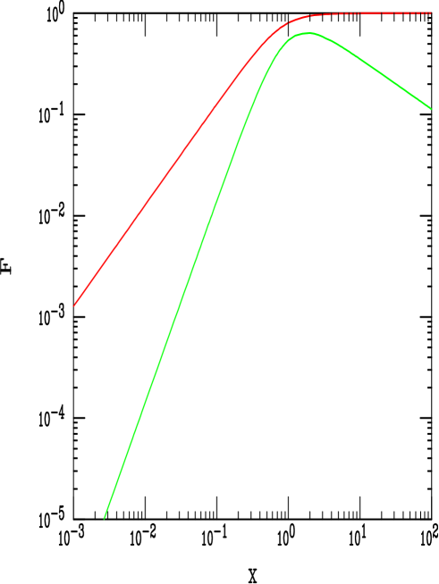
Figure 7: The form factors ${\cal G}$(upper curve) and ${\cal G}$’(lower curve) as discussed in the text for the case $n=1$.

6 Summary and Conclusions

In this paper we have begun a detailed examination of the predictions of the Universal Extra Dimensions model for future colliders. Since it is known from the detailed analysis of Appelquist, Cheng and Dobrescu and the subsequent work by Agashe, Deshpande and Wu that the compactification scale, $M_{c}$ in this model can be as low as 350 GeV, we first examined the contribution to $g-2$ in this model arising from loops of KK states. Although this contribution, of order $-40\times 10^{-11}$, may eventually be probed by the Brookhaven $g-2$ experiment, no new bounds on $M_{c}$ are at present obtainable. Next we turned to the production of the lightest KK states at lepton, $\gamma\gamma$ and hadron colliders. Here it was necessary to be reminded that due to tree-level conservation of KK number in the UED model it is necessary to pair-produce KK states. Since indirect searches for such states give rather poor reaches direct searches are of greater importance in this model than in the other cases discussed in the introduction. Thus to obtain interesting search reaches requires a hadron collider such as the Tevatron or LHC. Based on counting events we expect the reach st the Tevatron Run II (LHC) for KK states to be $\simeq 600(3000)$ GeV. Within the UED model itself these lightest KK states are stable even when loop corrections are included unless new interactions are introduced from elsewhere. If these states are indeed stable, the production of a large number of heavy stable charged particles would not be missed at either collider. It is more likely, however, that new physics does indeed enter rendering the KK modes unstable. In this paper we have examined three new physics scenarios that induce finite KK lifetimes and compared their decay signatures.

In the first case the UED model was embedded in a thick brane in a larger n-dimensional space in which gravity was free to propagate. Due to the difference in sizes over which the various fields are normalized, excited KK states can now decay to zero mode SM fields through the emission of gravitons whose rate is controlled by a geometric form-factor like function. At colliders this would appear as the production of pairs of SM states in association with a large amount of missing energy from the two towers of gravitons. In a second scenario, a ‘benign’ brane is introduced somewhere between the fixed points on which a set of non-renormalizable interactions occur. These interactions then induce mixing amongst the various KK levels violating KK number conservation and allowing excited KK modes to decay to SM fields. The branching fractions of all of the fermionic KK states were calculated while those of the gauge KK states are found to be essentially the same as the corresponding SM fields apart from phase space effects. In the last scenario we consider the possibility that the 5-dimensional fermion fields obtain a common bulk mass; a common bulk mass was assumed both on the basis of simplicity and to avoid any potentially dangerous FCNC. This modifies the wave-function of the zero modes so that a finite overlap exists with higher modes. This then allows the decay of KK states through another set of form-factors that arise from these wave function overlaps. Unfortunately these form-factors vanish for $Z_{2}$-odd KK excited states due to $Z_{2}$ parity conservation and thus these states will remain stable. In this scenario the decay signatures are found to be similar to those of the previous case.

Clearly, independent of whether the first excited KK modes are stable or decay through one of the above mechanisms, if the UED framework is at all correct future colliders will yield exciting signals of new physics associated with extra dimensions.

Acknowledgements

The author would like to thank H.-C Cheng and B. Dobrescu for discussions during the early stages of this work and the CERN Theory Division for its hospitality. The author would also like to thank H. Davoudiasl and J.L. Hewett for general discussions on models with extra dimensions.

References

- [1] See, for example, I. Antoniadis, Phys. Lett. B246, 377 (1990); I. Antoniadis, C. Munoz and M. Quiros, Nucl. Phys. B397, 515 (1993); I. Antoniadis and K. Benalki, Phys. Lett. B326, 69 (1994)and Int. J. Mod. Phys. A15, 4237 (2000); I. Antoniadis, K. Benalki and M. Quiros, Phys. Lett. B331, 313 (1994); K. Benalki, Phys. Lett. B386, 106 (1996); E. Accomando, I. Antoniadis and K. Benalki, Nucl. Phys. B579, 3 (2000).
- [2] See, for example, T.G. Rizzo and J.D. Wells, Phys. Rev. D61, 016007 (2000); P. Nath and M. Yamaguchi, Phys. Rev. D60, 116006 (1999); M. Masip and A. Pomarol, Phys. Rev. D60, 096005 (1999); W.J. Marciano, Phys. Rev. D60, 093006 (1999); L. Hall and C. Kolda, Phys. Lett. B459, 213 (1999); R. Casalbuoni, S. DeCurtis and D. Dominici, Phys. Lett. B460, 135 (1999); R. Casalbuoni, S. DeCurtis, D. Dominici and R. Gatto, Phys. Lett. B462, 48 (1999); A. Strumia, Phys. Lett. B466, 107 (1999); F. Cornet, M. Relano and J. Rico, Phys. Rev. D61, 037701 (2000); C.D. Carone, Phys. Rev. D61, 015008 (2000); A. Delgado, A. Pomarol and M. Quiros, J. High En. Phys. 0001, 030 (2000.)
- [3] N. Arkani-Hamed and M. Schmaltz, Phys. Rev. D61, 033005 (2000).
- [4] N. Arkani-Hamed, Y. Grossman and M. Schmaltz, Phys. Rev. D61, 115004 (2000); E.A. Mirabelli and M. Schmaltz, Phys. Rev. D61, 113001 (2000); G.C. Branco, A. De Gouvea and M.N. Rebolo, hep-ph/0012289.
- [5] T. Appelquist, H.-C. Cheng and B.A. Dobrescu, hep-ph/0012100. See also R. Barbieri, L.J. Hall and Y. Nomura, hep-ph/0011311.
- [6] The author would like to thank A. Strumia for this important observation.
- [7] K. Agashe, N.G. Deshpande and G.-H.Wu, hep-ph/0105084.
- [8] H. Davoudiasl, J.L. Hewett and T.G. Rizzo, Phys. Lett. B493, 135 (2000).
- [9] The magnitude of the contribution to in the UED model was briefly discussed in K. Agashe, N.G. Deshpande and G.-H.Wu, hep-ph/0103235.
- [10] S.J. Brodsky and J.D. Sullivan, Phys. Rev. 156, 1644 (1967) ; S.J. Brodsky and S. Drell, Phys. Rev. D22, 2236 (1980).
- [11] See, for example, A. Delgado, A. Pomarol and M. Quiros, Phys. Rev. D60, 095008 (1999).
- [12] H.N. Brown et al., Muon Collaboration, Phys. Rev. Lett. 86, 2227 (2001).
- [13] W.J. Marciano and B.L Roberts, hep-ph/0105056 and references therein.
- [14] As this paper was being completed a paper by T. Appelquist and B.A. Dobrescu, hep-ph/0106140, appeared which also has examined the of the muon in the UED model. While we agree on the sign and magnitude of their result, we differ by approximately a factor of 3. In either case, no new constraint on the UED model is obtained.
- [15] D.A. Dicus, C.D. McMullen and S. Nandi, hep-ph/0012259.
- [16] N. Arkani-Hamed, S. Dimopoulos, and G. Dvali, Phys. Lett. B429, 263 (1998), and Phys. Rev. D59, 086004 (1999); I. Antoniadis, N. Arkani-Hamed, S. Dimopoulos, and G. Dvali, Phys. Lett. B436, 257 (1998).
- [17] For a discussion of brane form factors, see A. DeRujula, A. Donini, M.B. Gavela and S. Rigolin, Phys. Lett. B482, 195 (2000).
- [18] G.F. Giudice, R. Rattazzi, and J.D. Wells, Nucl. Phys. B544, 3 (1999); T. Han, J.D. Lykken, and R.-J. Zhang, Phys. Rev. D59, 105006 (1999).