29 June 2001

JYFL-7/01

HIP-2001-26/TH

hep-ph/0106330

HEAVY ION COLLISION MULTIPLICITIES AND GLUON DISTRIBUTION FUNCTIONS

K.J. Eskola,^a,c, K. Kajantie^b, and K. Tuominen^a,

^a Department of Physics, University of Jyväskylä,
P.O.Box 35, FIN-40351 Jyväskylä, Finland
^b Department of Physics, University of Helsinki
P.O.Box 64, FIN-00014 University of Helsinki, Finland
^c Helsinki Institute of Physics,
P.O.Box 64, FIN-00014 University of Helsinki, Finland

Abstract

Atomic number ($A$) and energy ($\sqrt{s}$) scaling exponents of multiplicity and transverse energy in heavy ion collisions are analytically derived in the perturbative QCD + saturation model. The exponents depend on the small-$x$ behaviour of gluon distribution functions at an $x$-dependent scale. The relation between initial state and final state saturation is also discussed.

1 Introduction

New RHIC data on the multiplicity in Au+Au collisions [1] and its centrality dependence [2, 3] has given us new insight into the dynamics of ultrarelativistic heavy ion collisions. The data from central and nearly central collisions can be understood [4, 5] in terms of a conventional soft + hard two-component picture [6], but also in a dynamically more unified perturbative QCD + saturation model [7, 8].

The results of [7] are formulated in the form of scaling rules: quantity $\sim CA^{a}(\sqrt{s})^{b}$, where the constants $C,a,b$ are determined numerically for central A+A collisions using independently determined parton distribution functions [9] with shadowing [10]. For example, for the dominant saturation scale $p_{{\mbox{\scriptsize sat}}}$ and for the multiplicity $N$ per unit rapidity one finds:

$$p_{{\mbox{\scriptsize sat}}} = 0.208\,A^{0.128}\,\sqrt{s}^{\,0.191},$$ (1)

$$N(p_{{\mbox{\scriptsize sat}}}) = 1.383\,A^{0.922}\sqrt{s}^{\,0.383},$$ (2)

where $p_{{\mbox{\scriptsize sat}}}$ and $\sqrt{s}$ are in units of GeV. Thus the multiplicity $N\sim A^{0.922}$ instead of the exponent $N\sim A^{4/3}$ appropriate for hard collisions or $N\sim A$ appropriate for the saturation model if $xg(x)\sim$ const and $\alpha_{s}\sim$ const. Even more striking is the rather fast powerlike dependence $N\sim\sqrt{s}^{0.383}$, much faster than the $\sim\log(s)$ or $\sim\log^{2}(s)$ behaviour observed for pp collisions.

The results in (1)-(2) lead to rather definite and easily testable predictions for the overall magnitude and the $A$ and $\sqrt{s}$ dependencies of heavy ion experimental results. Agreement with the first RHIC results for the charged multiplicity and $\sqrt{s}$ dependence is good [1]. It would thus be of some value to derive the numerically computed scaling parameters analytically and to understand the underlying physics. It is the purpose of this note to carry out this derivation.

The dominant part of the analytic estimate is a derivation of an accurate approximation for hard production of minijets in pp collisions. This, of course, is a most standard problem, but with one important difference: as we are interested in the physics of heavy ion collisions in the RHIC-LHC energy range, $\sqrt{s}\,\raise 1.29167pt\hbox{$>$\kern-7.5pt\raise-4.73611pt\hbox{$\sim$}}\,100$ GeV, and for $A\sim 200$, we know the magnitudes of the dominant scales of the problem, $Q\sim p_{{\mbox{\scriptsize sat}}}$ and $x\sim p_{{\mbox{\scriptsize sat}}}/\sqrt{s}$. It is thus sufficient to find out an approximation for the gluon distribution functions in this range. In fact, we shall find that the very simple estimate $xg(x,Q^{2})\sim(Q/x)^{\delta}$ with $\delta\approx 0.5$ is quite accurate in the vicinity of the dominant scale $Q$, which depends on $x$. After obtaining an analytic approximation for the perturbative minijet cross section $d\sigma/dy(y=0,p_{T}\geq p_{0})$ (Section 2) it is straightforward to find the scaling exponents (Section 3).

The idea of saturation originates from [11, 12, 13] and is usually discussed in connection with small-$x$ behaviour of gluon distribution functions (“initial state saturation”). Here we have in mind rather a picture with the saturation of produced gluons (“final state saturation”). Using the analytic approximation we can show the close phenomenological relation of initial and final state saturation (Section 4). This close relation also follows from the fact that $N(p_{{\mbox{\scriptsize sat}}})$ is proportional to the initial state gluon distribution probed at the final state saturation scale. The analytic approximation can also be extended to models of local saturation (Section 5).

2 Analytic estimates of the minijet cross section

Consider first inclusive gluon production from the subprocess gg$\to$gg in pp collisions:

$${d\sigma\over dyd^{2}p_{T}}=K\int dy_{2}\,x_{1}g(x_{1},p_{T}^{2})\,x_{2}g(x_{2},p_{T}^{2}){9\alpha_{s}^{2}\over 2p_{T}^{4}}\left(1-{x_{T}^{2}\over 4x_{1}x_{2}}\right)^{3}.$$ (3)

Here $K$ describes the effect of higher order corrections [14] and the fractional momenta are $x_{1}={\frac{1}{2}}x_{T}(e^{y}+e^{y_{2}}),\,x_{2}={\frac{1}{2}}x_{T}(e^{-y}+e^{-y_{2}})$ with $x_{T}=2p_{T}/\sqrt{s}$. The integral is over $-\log(2/x_{T}-e^{-y})\leq y_{2}\leq\log(2/x_{T}-e^{y})$. The last factor in (3) is equal to $(1+2\cosh Y)^{3}/(2+2\cosh Y)^{3},\,\,Y=y-y_{2}$.

For the analytic estimates, we need to approximate the gluon distribution $xg(x,Q^{2})$ in a region which dominates the $p_{T}$- and $y_{2}$-integrations. From (2), we see that $p_{{\mbox{\scriptsize sat}}}\sim 1$ GeV at $\sqrt{s}=200$ GeV, and $p_{{\mbox{\scriptsize sat}}}\sim 2$ GeV at $\sqrt{s}=5500$ GeV for $A\sim 200$. In addition, as shown in Fig. 1 of [7], we know that about 90% of all the minijets produced above the saturation scale have transverse momenta $p_{{\mbox{\scriptsize sat}}}\leq p_{T}\,\,\raise 1.29167pt\hbox{$<$\kern-7.5pt\raise-4.73611pt\hbox{$\sim$}}\,\,2p_{{\mbox{\scriptsize sat}}}$. The scale in (3) is chosen as $Q=p_{T}$, so the relevant region in $Q$ thus is $1\dots 2$ GeV for $\sqrt{s}=200$ GeV and $2\dots 4$ GeV for $\sqrt{s}=5500$ GeV. In what follows, we shall fix $y=0$ in (3). This makes the integral even and it suffices to consider only the integration region $0\leq y_{2}\leq\log(2/x_{T}-1)$. The fractional momenta are now limited to $x_{T}/2\leq x_{1}\leq 1$ and $x_{T}/2\approx(2/x_{T}-1)^{-1}\leq x_{2}\leq x_{T}/2$. From the numerical computation of (3), we have checked that the dominant ($\geq 70$%) contribution comes from $y_{2}\,\raise 1.29167pt\hbox{$<$\kern-7.5pt\raise-4.73611pt\hbox{$\sim$}}\,4$ for $\sqrt{s}=5500$ GeV ($p_{T}\geq 2$ GeV), and from $y_{2}\,\raise 1.29167pt\hbox{$<$\kern-7.5pt\raise-4.73611pt\hbox{$\sim$}}\,3$ for $\sqrt{s}=200$ GeV ($p_{T}\geq 1$ GeV). In the analytic estimates we thus need to describe $xg(x,Q^{2})$ at $Q/\sqrt{s}\,\raise 1.29167pt\hbox{$<$\kern-7.5pt\raise-4.73611pt\hbox{$\sim$}}\,x\,\raise 1.29167pt\hbox{$<$\kern-7.5pt\raise-4.73611pt\hbox{$\sim$}}\,50Q/\sqrt{s}$ in the vicinity of $Q=2$ GeV for $\sqrt{s}=5500$ GeV and at $Q/\sqrt{s}\,\raise 1.29167pt\hbox{$<$\kern-7.5pt\raise-4.73611pt\hbox{$\sim$}}\,x\,\raise 1.29167pt\hbox{$<$\kern-7.5pt\raise-4.73611pt\hbox{$\sim$}}\,20Q/\sqrt{s}$ in the vicinity of $Q=1$ GeV for $\sqrt{s}=200$ GeV.

         

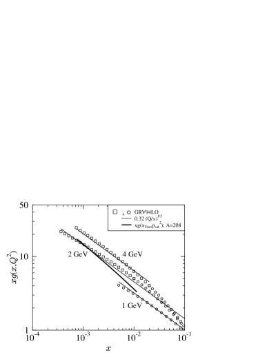
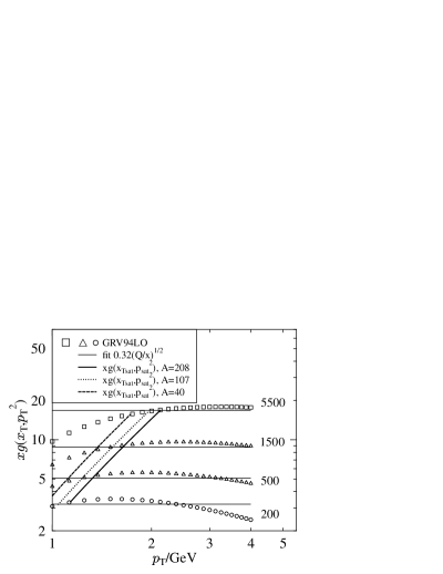
Figure 1: (a) The gluon distribution $xg(x,Q^{2})$ as a function of $x$ at fixed scales $Q$, plotted in the region which dominates minijet production at saturation at $\sqrt{s}=200...5500$ GeV, i.e. at $x\,\raise 1.1625pt\hbox{$>$\kern-6.75pt\raise-4.2625pt\hbox{$\sim$}}\,Q/\sqrt{s}$ with $Q=1$, 2 and 4 GeV (see the text for details). The squares and circles show the GRV94-LO distributions [9], the solid lines are the fit $xg(x,Q^{2})=0.32(Q/{\rm GeV}/x)^{0.5}$. The solid thick line shows the gluon density probed at saturation, $xg(x_{T{\rm sat}},p_{{\mbox{\scriptsize sat}}}^{2})$ with $A=208$ at $\sqrt{s}=200\dots 5500$ GeV. (b) The gluon distribution $xg(x_{T},p_{T}^{2})$ as a function of the scale $p_{T}$ for $\sqrt{s}=200$, 500, 1500 and 5500 GeV. The symbols are the GRV distributions and the thin solid lines are the fit. The thick curves (solid, dotted, dashed) are the gluon densities probed at saturation, $xg(x_{T{\rm sat}},p_{{\mbox{\scriptsize sat}}}^{2})$, at different $\sqrt{s}$ for $A=208$, 107 and 40, correspondingly. The region relevant for our problem is to the right of the thick curves.

The gluon distribution $xg(x,Q^{2})$ as obtained from the set GRV94-LO [9] in the $x,Q$ region discussed above is shown in Fig.1a. The symbols are for $\sqrt{s}=200$ GeV (circles) and for $\sqrt{s}=5500$ GeV (squares). For our purposes, and as the kinematic region is now limited, a simple power law $x^{-0.5}$, shown by the solid lines in Fig.1a, reproduces $xg$ adequately. To simulate the effect of pQCD scale evolution, we note from Fig.1b that in the dominant region (to the right of the thick tilted lines), $xg(x\sim p_{T}/\sqrt{s},p_{T}^{2})$ is approximately constant. This suggests a simple fit

$$xg(x,Q^{2})=C_{0}(\frac{Q/{\rm GeV}}{x})^{\delta},$$ (4)

with $\delta=0.5$ and $C_{0}=0.32$, as shown by the solid lines in Fig.1. Below we shall see that $N(p_{{\mbox{\scriptsize sat}}})\sim xg(x_{T{\rm sat}},p_{{\mbox{\scriptsize sat}}}^{2})$, with $x_{T{\rm sat}}=2p_{{\mbox{\scriptsize sat}}}/\sqrt{s}=0.416A^{0.128}(\sqrt{s}/{\rm GeV})^{-0.809}$, where the relation (1) is used. The gluon density probed at final saturation, $xg(x_{T{\rm sat}},p_{{\mbox{\scriptsize sat}}}^{2})$ is shown by the thick line in Fig. 1a for $A=208$ from $\sqrt{s}=200$ GeV to 5500 GeV. Note that on this curve each point in $x$ now corresponds to one $\sqrt{s}$ and one $p_{{\mbox{\scriptsize sat}}}$.

If a similar procedure is carried out for the CTEQ5 set of parton distribution functions [15], effectively the same result is obtained, the value of $C_{0}$ is decreased by less than 10% and $\delta\approx 0.47$ is somewhat smaller.

With the fit $xg(x,p_{T}^{2})=C_{0}(p_{T}/{\rm GeV}/x)^{\delta}$, ($\delta=0.5$, $C_{0}$=0.32), Eq. (3) can now be expressed as

$$\frac{d\sigma}{dyd^{2}p_{T}}=2\cdot K\frac{9\alpha_{\rm s}^{2}(p_{T}^{2})}{2p_{T}^{4}}[C_{0}(\frac{\sqrt{s}}{{\rm GeV}})^{\delta}]^{2}\sum_{n=0}^{3}(-1)^{n}\Big{(}{3\atop n}\Big{)}(\frac{1}{4})^{n+\delta}\int_{0}^{{{\scriptstyle\log(\sqrt{s}/p_{T}-1)}\atop~{}}\atop}dy_{2}\,\,[\cosh\frac{y_{2}}{2}]^{-2(n+\delta)}.$$ (5)

As our focus is at a region where $x_{T}\ll 1$, we write

$$\int_{0}^{{{\scriptstyle\log(\sqrt{s}/p_{T}-1)}\atop~{}}\atop}dy_{2}\,\,[\cosh\frac{y_{2}}{2}]^{-2\Delta} = \int_{0}^{\infty}\,dy_{2}\,[\cosh\frac{y_{2}}{2}]^{-2\Delta}-\int_{\atop{\atop{\scriptstyle\log(\sqrt{s}/p_{T}-1)}}}^{\infty}dy_{2}\,[\cosh\frac{y_{2}}{2}]^{-2\Delta}$$ (6)

$$= B(\Delta,\frac{1}{2})-2^{\Delta}\int_{0}^{x_{T}}dzz^{\Delta-1}(1-\frac{z}{2})^{\Delta-1}$$ (7)

$$= B(\Delta,\frac{1}{2})+(\frac{x_{T}}{2})^{\Delta}\sum_{k=0}^{\infty}\bigg{(}{\Delta-1\atop k}\bigg{)}\frac{1}{k+\Delta}(-\frac{x_{T}}{2})^{k},$$ (8)

where $B(\Delta,\frac{1}{2})$ is the beta function, $\Delta=n+\delta$, and in the second integral a change of integration variable from $y_{2}$ to $z=x_{T}/x_{1}$ has been made. In the limit of small $x_{T}$, the leading term for each $n$ is given by the first term with the beta function. The $p_{T}$ distribution thus becomes

$$\frac{d\sigma}{dyd^{2}p_{T}}=2\cdot K\frac{9\alpha_{\rm s}^{2}(p_{T}^{2})}{2p_{T}^{4}}[C_{0}(\frac{\sqrt{s}/{\rm GeV}}{2})^{\delta}]^{2}B(\delta,\frac{1}{2})a(\delta)+{\cal O}(x_{T}^{\delta})$$ (9)

where

$$a(\delta)=1-\frac{3}{4}\frac{\delta}{\frac{1}{2}+\delta}+\frac{3}{4^{2}}\frac{\delta(\delta+1)}{(\frac{1}{2}+\delta)(\frac{3}{2}+\delta)}-\frac{1}{4^{3}}\frac{\delta(\delta+1)(\delta+2)}{(\frac{1}{2}+\delta)(\frac{3}{2}+\delta)(\frac{5}{2}+\delta)}\stackrel{{\scriptstyle\scriptstyle\delta=0.5}}{{\approx}}0.6904$$ (10)

and

$$B(\delta,\frac{1}{2})=\frac{\sqrt{\pi}\Gamma(\delta)}{\Gamma(\frac{1}{2}+\delta)}\stackrel{{\scriptstyle\scriptstyle\delta=0.5}}{{=}}\pi$$ (11)

Notice that now, in (9), $[C_{0}(\frac{\sqrt{s}/{\rm GeV}}{2})^{\delta}]^{2}=[xg(x_{T},p_{T}^{2})]^{2}$ appears.

Integration over $p_{T}$ then gives the minijet cross section

$$2\sigma_{\mbox{\scriptsize pQCD}}(p_{0})\approx{d\sigma\over dy}\bigg{|}_{y=0\atop p_{0}} \approx \int_{p_{0}}^{\infty}2\pi p_{T}dp_{T}{d\sigma\over dyd^{2}p_{T}}$$ (12)

$$\approx 2\cdot K\frac{9\pi}{2}B(\delta,\frac{1}{2})a(\delta)[xg(x_{T0},p_{0}^{2})]^{2}{\cal I}(p_{0}^{2}),$$ (13)

where

$${\cal I}(p_{0}^{2})\equiv\int_{p_{0}^{2}}^{\infty}dp_{T}^{2}\frac{\alpha_{s}^{2}(p_{T}^{2})}{(p_{T}^{2})^{2}}=\frac{\alpha_{s}^{2}(p_{0}^{2})}{p_{0}^{2}}\log\frac{p_{0}^{2}}{\Lambda_{\rm QCD}^{2}}\bigg{[}1-\frac{p_{0}^{2}}{\Lambda_{\rm QCD}^{2}}\log\frac{p_{0}^{2}}{\Lambda_{\rm QCD}^{2}}E_{1}(\log\frac{p_{0}^{2}}{\Lambda_{\rm QCD}^{2}})\bigg{]}$$ (14)

where $E_{1}(z)$ is the exponential integral and the running coupling $\alpha_{s}(Q^{2})$ is that to one loop. Denoting $z=\log(p_{0}^{2}/\Lambda_{\rm QCD}^{2})$ and using the approximation [16]

$$z{\rm e}^{z}E_{1}(z)=\frac{z^{2}+a_{1}z+a_{2}}{z^{2}+b_{1}z+b_{2}}+\epsilon(z)$$ (15)

where $|\epsilon(z)|<5\cdot 10^{-5}$, $a_{1}=2.334733$, $a_{2}=0.250621$, $b_{1}=3.330657$ and $b_{2}=1.681534$, we arrive at the following expression for the hard cross section at central rapidity:

$$\frac{d\sigma}{dy}\bigg{|}_{y=0\atop p_{0}}\approx 2K\frac{9\pi}{2}B(\delta,\frac{1}{2})a(\delta)\cdot f(\log\frac{p_{0}^{2}}{\Lambda_{\rm QCD}^{2}})\frac{\alpha_{s}^{2}(p_{0}^{2})}{p_{0}^{2}}[xg(x_{T0},p_{0}^{2})]^{2},$$ (16)

where $f(z)=({0.995924z+1.430913})/({z+3.330657+1.681534/z})$, $x_{T0}=2p_{0}/\sqrt{s}$ and $xg(x_{T0},p_{0}^{2})=C_{0}(\frac{\sqrt{s}/{\rm GeV}}{2})^{\delta}$. Setting $f(z)=1$ would correspond to the approximation $\alpha_{s}(p_{T}^{2})=\alpha(p_{0}^{2})$ in the integral in Eq. (14).

As anticipated based on the precision of the rough fit to $xg$, our analytic estimate (16) reproduces the “exact” numerical result (with gluons only, no shadowing) to about 10% accuracy near $p_{0}=2$ GeV at $\sqrt{s}=5500$ GeV. An improved accuracy would require a better fit to $xg(x,Q^{2})$ in the regions of large $y_{2}$(large $x_{1}$). The terms ${\cal O}(\sqrt{x_{T0}/2})$, now neglected, contribute only at the level of a few percent at $\sqrt{s}=5500$ GeV, $p_{0}=2$ GeV, and at a level of 10% at $\sqrt{s}=200$ GeV, $p_{0}=1$ GeV. Since the main emphasis here is to understand the origin of the scaling exponents, we leave the overall normalization as a rough estimate.

To extract the $A$ and $\sqrt{s}$ scaling exponents for the saturation scale analytically, we introduce a second parameter $\xi$ by noting that the complicated $p_{0}$ dependence of the product $\alpha_{s}^{2}f$ in (16) can, in the relevant range, to good accuracy be represented by a power:

$$\alpha_{s}(p_{0}^{2})\sqrt{f(\log(p_{0}^{2}/\Lambda_{\rm QCD}^{2}))}\approx D(\Lambda_{\rm QCD}/p_{0})^{\xi},$$ (17)

where $D=0.775$ and $\xi=0.444$ (with $\Lambda_{\rm QCD}=0.2$ GeV and $N_{f}=4$). The accuracy of this approximation is within 1.5 % in the region $p_{0}=1\dots 2$ GeV.

Also the first $p_{T}$-moment of the $p_{T}$-distribution can be computed by using the same sequence of approximations as above. The result is

$$\sigma_{\rm pQCD}\langle E_{T}\rangle \approx {d\sigma\over dy}\langle p_{T}\rangle\bigg{|}_{y=0\atop p_{0}}\approx\int_{p_{0}}^{\infty}2\pi p_{T}dp_{T}{d\sigma\over dyd^{2}p_{T}}\cdot p_{T}$$ (18)

$$\approx 2K\frac{9\pi}{2}B(\delta,\frac{1}{2})a(\delta)\cdot 2f(\log\frac{p_{0}}{\Lambda_{\rm QCD}})\frac{\alpha_{s}^{2}(p_{0})}{p_{0}}[xg(x_{T0},p_{0}^{2})]^{2},$$ (19)

where now the same function $f$ appears as in Eq. (16) but with a different argument. For the average $p_{T}$, we thus get

$$\langle p_{T}\rangle\bigg{|}_{y=0\atop p_{0}}\approx\frac{2f(\log(p_{0}/\Lambda_{\rm QCD}))}{f(\log(p_{0}^{2}/\Lambda_{\rm QCD}^{2}))}\cdot p_{0}\approx F\cdot\bigg{(}\frac{p_{0}}{\Lambda_{\rm QCD}}\bigg{)}^{\eta}\cdot p_{0}$$ (20)

where in the last step the power law approximation again holds in the region $p_{0}=1\dots 2$ GeV and $\eta=0.0624$ and $F=1.399$.

3 The scaling exponents

We can now apply the analytic approximations (16) and (17) to the minijet cross section (13) in the final state saturation condition [7] for central $A$+$A$ collisions:

$$N(p_{0})=T_{AA}(\mbox{\bf b}=0)\,2\sigma_{\mbox{\scriptsize pQCD}}(p_{0})=p_{0}^{2}R_{A}^{2}.$$ (21)

Saturation is a dynamic phenomenon and, in the weak coupling limit, there would be powers of $\alpha_{s}$ together with various numerical constants in (21). Taking a constant value $\approx 0.3$ for $\alpha_{s}$ the net effect in (21) is an overall constant of about 1. Even at the LHC one is most likely far from the weak coupling region and we shall not keep the coupling constant dependence in the right hand side of (21) explicitly. This approximation is in agreement with RHIC data. Note, however, that $\alpha_{s}$ is kept in (16).

Using $T_{AA}(0)=A^{2}/(\pi R_{A}^{2})$ with $R_{A}\approx 1.12A^{1/3}$ and Eq. (16) in the power-law approximation (17), one finds that the solution of (21) is

$$p_{{\mbox{\scriptsize sat}}}\approx\bigg{[}\frac{3\sqrt{B(\delta,\frac{1}{2})a(\delta)}}{1.12^{2}\cdot({\rm fm}\cdot{\rm GeV})^{2}}\cdot C_{0}(\frac{1}{2})^{\delta}\cdot D\cdot\Lambda_{\rm QCD}^{\xi}\bigg{]}^{1/(2+\xi)}K^{1/(4+2\xi)}A^{1/(6+3\xi)}{\sqrt{s}}^{\delta/(2+\xi)},$$ (22)

where now the origin of each factor can be easily traced down. The exponent $\delta$ comes from the behaviour of the gluon structure function in Eq. (4) whereas the exponent $\xi$ originates from the running of the strong coupling constant in Eq. (17). The numerical value of the constant in front of the $K$-factor is 0.1625. It is also understood that $p_{{\mbox{\scriptsize sat}}}$, $\Lambda_{\rm QCD}$ and $\sqrt{s}$ are in units of GeV. We have also kept $K$ separate to show how $p_{{\mbox{\scriptsize sat}}}$ and, especially, $N(p_{{\mbox{\scriptsize sat}}})$ depend on it. The initial multiplicity of produced gluons at saturation, $N(p_{{\mbox{\scriptsize sat}}})=p_{{\mbox{\scriptsize sat}}}^{2}R_{A}^{2}$, then is

$$N(p_{{\mbox{\scriptsize sat}}})\approx 0.850\cdot K^{1/(2+\xi)}A^{(6+2\xi)/(6+3\xi)}{\sqrt{s}}^{2\delta/(2+\xi)}$$ (23)

Note that the dependence on the $K$ factor is rather weak, $N(p_{{\mbox{\scriptsize sat}}})\sim K^{0.41}$ – instead of $\sim K$. Substituting the numerical values for the coefficients $C_{0}$ and $D$, and for the exponents $\delta$ and $\xi$ as discussed above, and $K=2$ as in [7], we obtain the following scaling laws:

$$p_{{\mbox{\scriptsize sat}}} \approx 0.187A^{0.136}\sqrt{s}^{\,0.205},$$ (24)

$$N(p_{{\mbox{\scriptsize sat}}}) \approx 1.13A^{0.939}\sqrt{s}^{\,0.409}.$$ (25)

Since the numerical results in Eqs. (1) and (2) contain shadowing, which is not included in the analytic estimates above, we should compare the scaling laws obtained above with the ones obtained numerically without shadowing (all parton flavours included):

$$p_{{\mbox{\scriptsize sat}}} = 0.193\,A^{0.137}\,\sqrt{s}^{\,0.204},$$ (26)

$$N(p_{{\mbox{\scriptsize sat}}}) = 1.20\,A^{0.941}\sqrt{s}^{\,0.408}.$$ (27)

The agreement is good and we have thus analytically understood how these scaling laws arise.

The numerical result for the CTEQ5 set [15] (no shadowing) is $p_{{\mbox{\scriptsize sat}}}=0.208\,A^{0.141}\,\sqrt{s}^{\,0.192}$, $N(p_{{\mbox{\scriptsize sat}}})=1.37\,A^{0.952}\sqrt{s}^{\,0.384}$. The somewhat slower $\sqrt{s}$ dependence follows from a somewhat slower evolution in this set, $\delta\approx 0.47$.

Based on Eqs. (21) and (16) the multiplicity of produced gluons at saturation can also be cast in the form

$$N(p_{{\mbox{\scriptsize sat}}})\approx\sqrt{K9B(\delta,{\scriptstyle\frac{1}{2}})a(\delta)}\sqrt{f(\log{(p_{{\mbox{\scriptsize sat}}}^{2}/\Lambda_{\rm QCD}^{2})})}\,\alpha_{s}(p_{{\mbox{\scriptsize sat}}}^{2})\,A\,xg(x_{\rm Tsat},p_{{\mbox{\scriptsize sat}}}^{2})$$ (28)

Thus we see that the initial multiplicity of produced gluons directly probes the gluon distribution at the saturation scale, as derived in [13] for initial state saturation. The powers of $\alpha_{s}$ are not the same because they differ already in the saturation condition (21).

Nuclear shadowing effects can also be discussed in the analytic approximation. Overall they are a fairly small correction to the results above: the numerical evaluation of $N(p_{{\mbox{\scriptsize sat}}})$ with the EKS98 shadowing [10] shows a 16 % reduction at $\sqrt{s}=5500$ GeV and a 7 % reduction at $\sqrt{s}=200$ GeV for $A=208$. For smaller nuclei the effects are smaller. Shadowing obviously slightly decreases the effective exponent $\delta$ in an $A$-dependent way. The dependence of the factor $\sqrt{B(\delta,{\scriptstyle\frac{1}{2}})a(\delta)}$ on $A$ remains, however, small. Disregarding the few percent effects from the factor $\sqrt{f(\log{(p_{{\mbox{\scriptsize sat}}}^{2}/\Lambda_{\rm QCD}^{2})})}$, we arrive at the following simple scaling for the multiplicity of produced gluons at saturation

$$N(p_{{\mbox{\scriptsize sat}}})\sim A\alpha_{s}(p_{{\mbox{\scriptsize sat}}}^{2})xg_{A}(x_{\rm Tsat},p_{{\mbox{\scriptsize sat}}}^{2}),$$ (29)

where now $p_{{\mbox{\scriptsize sat}}}$ is from Eq. (1) and $xg_{A}$ is the shadowed gluon distribution per nucleon. This result is tested against a full calculation of Eq. (2) in Fig. 3. The agreement with the numerically obtained results is good in the scalings with both $\sqrt{s}$ and $A$, especially at large $\sqrt{s}$ and large $A$. If the initial state multiplicity is directly proportional to the final state multiplicity, the measured charged particle multiplicity then directly probes the nuclear gluon distributions at the (final state) saturation scale.

Figure 2: The initial multiplicity of produced gluons $N(p_{{\mbox{\scriptsize sat}}})$ at saturation as a function of $\sqrt{s}$. The symbols are the numerically obtained fits, Eq. (2) with shadowing included (filled symbols), and Eq. (27) with no shadowing (open symbols). Circles, boxes and diamonds stand for $A=208$, 107 and 40, correspondingly. The solid curves are the prediction of Eq. (29), with $p_{{\mbox{\scriptsize sat}}}$ computed from the numerical fits, Eqs. (1) and (26) and with GRV94LO gluon densities with and without shadowing. The solid curves are normalised to the numerically obtained result for $A=208$ at $\sqrt{s}=5500$ GeV. The dashed curve shows the small effect of the term $f(\log(p_{{\mbox{\scriptsize sat}}}^{2}/\Lambda_{\rm QCD}^{2}))$.

Using the power-law approximation of Eq. (20), we obtain the average initial transverse energy per produced particle

$$\frac{E_{T}(p_{{\mbox{\scriptsize sat}}})}{N(p_{{\mbox{\scriptsize sat}}})} = \frac{T_{AA}(0)\sigma_{\rm pQCD}\langle E_{T}\rangle}{T_{AA}(0)2\sigma_{\rm pQCD}}\approx\langle p_{T}\rangle\bigg{|}_{y=0,p_{{\mbox{\scriptsize sat}}}}\approx 1.546\bigg{(}\frac{p_{{\mbox{\scriptsize sat}}}}{{\rm GeV}}\bigg{)}^{\eta}\cdot p_{{\mbox{\scriptsize sat}}}.$$ (30)

From here, using the analytic approximation for $p_{{\mbox{\scriptsize sat}}}$ from Eq. (22) and $N(p_{{\mbox{\scriptsize sat}}})=p_{{\mbox{\scriptsize sat}}}^{2}R_{A}^{2}$, we get

$$E_{T}(p_{{\mbox{\scriptsize sat}}}) = 0.191K^{(3+\eta)/(4+2\xi)}A^{2/3+(3+\eta)/(6+3\xi)}\sqrt{s}^{\delta(3+\eta)/(2+\xi)}$$ (31)

$$= 0.191K^{0.627}A^{1.08}\sqrt{s}^{0.626}.$$ (32)

At saturation, the initial number and energy densities become

$$n_{i}={N(p_{{\mbox{\scriptsize sat}}})\over V(p_{{\mbox{\scriptsize sat}}})}={1\over\pi}p_{{\mbox{\scriptsize sat}}}^{3},\quad\epsilon_{i}={E_{T}(p_{{\mbox{\scriptsize sat}}})\over V(p_{{\mbox{\scriptsize sat}}})}=p_{{\mbox{\scriptsize sat}}}^{4}{1.546\over\pi}\bigg{(}\frac{p_{{\mbox{\scriptsize sat}}}}{{\rm GeV}}\bigg{)}^{0.0624},\,\,\,V(p_{{\mbox{\scriptsize sat}}})=\pi R_{A}^{2}/p_{{\mbox{\scriptsize sat}}}.$$ (33)

For a thermalised system of massless bosons at an energy density $\epsilon_{\rm th}=\epsilon_{i}$, the ratio initial energy per particle can be written as

$$\frac{\epsilon_{\rm th}}{n_{\rm th}}=2.7T=2.7\bigg{(}\frac{30\epsilon_{i}}{16\pi^{2}}\bigg{)}^{1/4}\approx\frac{E_{T}(p_{{\mbox{\scriptsize sat}}})}{N(p_{{\mbox{\scriptsize sat}}})}\cdot 0.97\bigg{(}\frac{p_{{\mbox{\scriptsize sat}}}}{{\rm GeV}}\bigg{)}^{-0.047},$$ (34)

which is indeed very close to the computed ratio $E_{T}(p_{{\mbox{\scriptsize sat}}})/N(p_{{\mbox{\scriptsize sat}}})=\epsilon_{i}/n_{i}$, independent of $A$ and $\sqrt{s}$ [7]. Since the system looks thermal from the point of view of the average quantities, rapid thermalisation is plausible. This is to be contrasted with the classical field approach [17] where it is found [18, 19] that the ratio $E_{T}/N$ is approximately three times larger, and therefore one might expect that thermalisation takes longer to achieve. On the other hand, from the analytic classical field calculation of Kovchegov [20] one infers that the $\epsilon/n$ ratio is very close to the thermal one [21] and, again, rapid thermalisation would be expected.

4 Final vs. initial state saturation

Usually saturation is discussed as a small-$x$ property of parton distribution functions. The above computations have been formulated referring to saturation of final state partons. One clearly has to understand the relation between these two approaches.

An initial state saturation scale $Q_{{\mbox{\scriptsize sat}}}$ can naturally be defined [22] as the gluon transverse area density including all gluons with $x>x_{\mbox{\scriptsize sat}}=2Q_{{\mbox{\scriptsize sat}}}/\sqrt{s}$:

$${N_{g}\over\pi R_{A}^{2}}={A\over\pi R_{A}^{2}}\int_{x_{\mbox{\scriptsize sat}}}^{1}\,dy\,g(y,Q_{{\mbox{\scriptsize sat}}}^{2})={A\over\pi R_{A}^{2}}C_{0}\delta^{-1}(Q_{{\mbox{\scriptsize sat}}}/{\rm{GeV}})^{\delta}x_{\mbox{\scriptsize sat}}^{-\delta}={1\over\pi}Q_{{\mbox{\scriptsize sat}}}^{2},$$ (35)

where the second equality was obtained by approximating $xg(x,Q^{2})=C_{0}(Q/{\rm GeV}/x)^{\delta}$ as before in Eq.(4). This equation is geometric and thus analogous to the saturation condition (21). In the parametric weak coupling limit also this equation would contain various group theory factors and powers of the coupling constant. As already discussed, we set them equal to unity in this work. As noted below Eq. (28), the powers of $\alpha_{s}$ in the saturation condition will affect the parametric dependence of e.g. multiplicity on $\alpha_{s}$.

Approximating the gluon distribution as earlier and solving $Q_{{\mbox{\scriptsize sat}}}$ from Eq. (35) gives almost the same A- and $\sqrt{s}$-scaling exponents as in (22) for $p_{{\mbox{\scriptsize sat}}}$, only the constant is somewhat different and the $K$-factor is absent:

$$Q_{{\mbox{\scriptsize sat}}} = \frac{1}{{\rm{fm\cdot GeV}}}(\frac{C_{0}}{2^{\delta}\delta})^{1/2}(\frac{A}{R_{A}^{2}})^{1/2}\sqrt{s}^{\delta/2}\sim A^{1/3}\sqrt{s}^{\delta/2},$$ (36)

where $Q_{{\mbox{\scriptsize sat}}}$ and $\sqrt{s}$ are in units of GeV and $R_{A}$ in fm. Note that it is essential that $Q_{{\mbox{\scriptsize sat}}}$ be both in the lower limit and on the right hand side of Eq.(35). The constant anyway is not uniquely defined, since the lower limit in (35) is not unique. Thus

$$p_{{\mbox{\scriptsize sat}}}\approx Q_{{\mbox{\scriptsize sat}}}.$$ (37)

In fig. (3) we plot the determination of the saturation scale using both final multiplicity and initial gluon distribution. From this figure we can see the small difference between the $\sqrt{s}$-scaling in $p_{{\mbox{\scriptsize sat}}}$ and $Q_{{\mbox{\scriptsize sat}}}$.

In the initial state saturation -picture the multiplicity $N$ of produced gluons is expected to be proportional to $N_{g}$ in Eq. (35), i.e.

$$N\sim N_{g}\sim Q_{{\mbox{\scriptsize sat}}}^{2}R_{A}^{2}$$ (38)

This relation is described in terms of the “parton liberation” constant in [23], and has been confirmed in the lattice simulations of the classical fields [19].

These results suggest that finding dynamical saturation of gluon distribution functions in a nucleus, one should also find saturation of produced gluons, the two phenomena are intimately related.

         

Figure 3: Solution of the saturation scale obtained by using the final multiplicity (solid lines) and Eq. (21), or the initial gluon multiplicity (dashed lines) and Eq. (35). The saturation scale is given by the intersection of these curves with the dotted line ’saturation’ corresponding to $p_{0}^{2}R_{A}^{2}$. Upper two curves correspond to LHC energy while the lower two correspond to the full RHIC energy. Neither multiplicity contains shadowing and $A=197$ on all curves. The dashed curves could be compared with those in Fig.2 of [22].

5 Local saturation

In [8] the criterion (21) was generalized to a local condition for transverse saturation of produced gluons in a collision with impact parameter b:

$$\frac{dN}{d\mbox{\bf s}}=T_{A}(\mbox{\bf s})T_{A}(\mbox{\bf b}-\mbox{\bf s})2\sigma_{\mbox{\scriptsize pQCD}}(p_{{\mbox{\scriptsize sat}}})=\frac{1}{\pi}p_{{\mbox{\scriptsize sat}}}^{2}(\mbox{\bf b},\mbox{\bf s}),$$ (39)

where s is the transverse coordinate; see also [24]. Using Eq.(16) in (39) one finds that exactly the same $A$ and $\sqrt{s}$ scaling exponents are obtained as from Eq.(21), and that the dependence on impact parameter and transverse coordinates is isolated into a product of nuclear density functions with a $\xi$-dependent exponent:

$$p_{{\mbox{\scriptsize sat}}}^{2}(\mbox{\bf b},\mbox{\bf s})\sim K^{1/(2+\xi)}\sqrt{s}^{2\delta/(2+\xi)}[T_{A}(\mbox{\bf s})T_{A}(\mbox{\bf b}-\mbox{\bf s})]^{1/(2+\xi)}$$ (40)

and

$$N(\mbox{\bf b})\sim\frac{1}{\pi}K^{1/(2+\xi)}\sqrt{s}^{2\delta/(2+\xi)}\int d^{2}\mbox{\bf s}[T_{A}(\mbox{\bf s})T_{A}(\mbox{\bf b}-\mbox{\bf s})]^{1/(2+\xi)}.$$ (41)

Again, $\delta=0.5$ and the parameter $\xi$ as given by Eq.(17) reproduce the behaviour of $N(\mbox{\bf b})$ obtained in the numerical computation in [8].

With our ansatz (4) for $xg(x,Q^{2})$, and neglecting the $p_{0}$-dependence of $f(\log p_{0}^{2}/\Lambda_{\rm QCD}^{2})$ in Eq. (16), Eq. (39) can also be cast into the form

$$p_{\mbox{\scriptsize sat}}^{2}(\mbox{\bf b},\mbox{\bf s})\sim K^{1/2}[T_{A}(\mbox{\bf s})T_{A}(\mbox{\bf b}-\mbox{\bf s})]^{1/2}\alpha_{s}xg(x,p_{{\mbox{\scriptsize sat}}}^{2}(\mbox{\bf b},\mbox{\bf s}))$$ (42)

and, consequently,

$$N(\mbox{\bf b})\sim K^{1/2}\int d^{2}\mbox{\bf s}[T_{A}(\mbox{\bf s})T_{A}(\mbox{\bf b}-\mbox{\bf s})]^{1/2}\alpha_{s}xg(x,p_{{\mbox{\scriptsize sat}}}^{2}(\mbox{\bf b},\mbox{\bf s})),$$ (43)

where $x=2p_{{\mbox{\scriptsize sat}}}(\mbox{\bf b},\mbox{\bf s})/\sqrt{s}$.

Eqs.(42) and (43) permit us to comment on the relation to [5], where it was postulated that the average (over s) saturation scale $Q_{\mbox{\scriptsize s}}^{2}$ (at fixed $b$) be proportional to the average (over s) transverse density of participating nucleons,

$$Q_{\mbox{\scriptsize s}}^{2}=\frac{8\pi^{2}\alpha_{s}N_{\mbox{\scriptsize c}}}{N^{2}_{\mbox{\scriptsize c}}-1}xg(x,Q_{\mbox{\scriptsize s}}^{2})\frac{\rho_{\mbox{\scriptsize part}}}{2}.$$ (44)

This leads to a total multiplicity, at fixed $b$,

$$\frac{dN}{d\eta}=cN_{\mbox{\scriptsize part}}xg(x,Q_{\mbox{\scriptsize s}}^{2}),$$ (45)

with $c\,\raise 1.29167pt\hbox{$>$\kern-7.5pt\raise-4.73611pt\hbox{$\sim$}}\,1,\,x=2Q_{\mbox{\scriptsize s}}/\sqrt{s}$. Also, the quantity $N/N_{\mbox{\scriptsize part}}$ is a slightly increasing function of $N{\mbox{\scriptsize part}}$ due to assumed scale evolution of the gluon structure function of the type $xg(x,Q^{2}_{\mbox{\scriptsize s}})\sim\ln(Q_{\mbox{\scriptsize s}}/\Lambda_{\rm QCD})$. The difference between [5] and [8] can be traced down to two points: First, to a slightly different dependence of the saturation scale on the transverse coordinate originating from $\rho_{\mbox{\scriptsize part}}\leftrightarrow[T_{A}(\mbox{\bf s})T_{A}(\mbox{\bf b}-\mbox{\bf s})]^{1/2}$. Second, to a different order of averaging to obtain $N(\mbox{\bf b})$, namely $N_{\mbox{\scriptsize part}}xg(x,Q_{\mbox{\scriptsize s}}^{2})\leftrightarrow\int d^{2}\mbox{\bf s}[T_{A}(\mbox{\bf s})T_{A}(\mbox{\bf b}-\mbox{\bf s})]^{1/2}\alpha_{s}xg(x,p_{{\mbox{\scriptsize sat}}}^{2}(\mbox{\bf b},\mbox{\bf s}))$.

6 Discussion

We have here shown how the $A$- and $\sqrt{s}$-scaling exponents and the overall magnitude of various global quantities in ultrarelativistic $A+A$ collisions, numerically computed in [7], can be simply related to two parameters, $\delta$ and $\xi$. The former (Eq.(4)) is related to the $x^{-\delta}$ behaviour at small-$x$ of the gluon distribution function at an effectively $x$-dependent saturation scale. Due to the interdependence of $x$ and $Q$ this is not the standard BFKL exponent describing small-$x$ behaviour at fixed scale $Q$. The parameter $\xi$ (Eq.(17)) approximates a complicated function containing $\alpha_{s}$ by a power. All the exponents are accurately reproduced by $\delta\approx 0.5,\,\,\xi=0.44$. The consequences of initial and final state saturation were also shown to be quantitatively similar.

One may note the following:

• The $A$-dependence of $N$ is not that of independent hard scatterings ($\sim A^{4/3}$), nor that of the saturation model with scaling cross section $\sigma_{\mbox{\scriptsize pQCD}}\sim 1/p_{0}^{2}$ ($\sim A$) but, due to powerlike non-scaling of $\sigma_{\mbox{\scriptsize pQCD}}$ even slower, $\sim A^{(6+2\xi)/(6+3\xi)}\sim A^{0.94}$. This is so even without shadowing, which further slightly reduces the exponent. A qualitative effect of this is that in the study of multiplicity per 0.5 times number of participants at some impact parameter b (which is the number to use to compare A+A data at various b with pp collisions) one obtains a curve decreasing very slowly with $N_{\mbox{\scriptsize part}}$ [4]. In fact, using the simple estimate $A_{\mbox{\scriptsize eff}}=0.5N_{\mbox{\scriptsize part}}(\mbox{\bf b})$, Eq.(23) implies that

  $${dN_{\mbox{\scriptsize ch}}/dy\over 0.5N_{\mbox{\scriptsize part}}}={\frac{2}{3}}\cdot 0.9\cdot 0.8503\cdot K^{1/(2+\xi)}(0.5N_{\mbox{\scriptsize part}})^{-\xi/(6+3\xi)}{\sqrt{s}}^{2\delta/(2+\xi)}.$$ (46)

  The decrease is thus very slow, $\sim N_{\mbox{\scriptsize part}}^{-0.06}$ for $\xi=0.444$. A more accurate analysis, using a local saturation condition [8], leads to a virtually constant (b-independent) ratio at RHIC and slightly increasing ratio at LHC, as shown in Fig.4.

  

  Figure 4: Rapidity density of charged particles near $y=0$ per 0.5 times the number of participants at LHC and RHIC energies computed using the local saturation criterion in [8]. RHIC data at $\sqrt{s}$ = 130 GeV [2] (open squares) and p+p rapidity densities (then $N_{\mbox{\scriptsize part}}=2$; arrows) are also shown. Large (small) $N_{\mbox{\scriptsize part}}$ corresponds to central $\mbox{\bf b}=0$ (peripheral, $\mbox{\bf b}\to 2R_{A}$) collisions.

• The energy dependence of $N$ and also of the ratio $N_{\mbox{\scriptsize ch}}/(0.5N_{\mbox{\scriptsize part}})$ is the powerlike $\sqrt{s}^{\,2\delta/(2+\xi)}\approx\sqrt{s}^{\,0.41}$ for $\delta=0.5,\,\xi=0.44$. This simple power behaviour follows from the numerically accurate power approximation (17). This $\sqrt{s}$ dependence is roughly verified at RHIC for $\sqrt{s}=56,130$ GeV and a new check is soon obtained with data at $\sqrt{s}=200$ GeV. At RHIC energies A+A collisions ($A=197$), have $N_{\mbox{\scriptsize ch}}/(0.5N_{\mbox{\scriptsize part}})\approx 3$, clearly but not strikingly larger than the value of $\approx$ 2 for p+p collisions. At LHC the increase would be from 5 for p+p to about 13 for A+A (Fig.4), a really striking effect, which will directly probe the behaviour of the nuclear gluon densities at small values of $x$.

• As noted previously, the powers of $\alpha_{s}$ appearing in the formulae for the multiplicity of produced gluons, Eqs. (28) and (29), will be affected by additional powers of $\alpha_{s}$ in the saturation condition (21), which will appear in the weak coupling limit but which were replaced by constants in this study covering a limited energy range. However, it is interesting to note that the exponent $\delta$ of the structure function appears only (at least when shadowing is neglected) in the $\sqrt{s}$-scaling. The $A$-scaling of the multiplicity depends only on the exponent $\xi$, which is related to $\alpha_{s}$. Including explicitly additional powers of $\alpha_{s}$ in the saturation condition (21), the $\xi$ dependence of $A$-scaling would change, and therefore the experimental measurement of $A$-scaling of the multiplicity would be a measurement of the actual form of the saturation criterion itself. Inclusion of, say, a factor $1/\alpha_{s}^{2}$, would make the $\alpha_{s}$ dependence of multiplicity of Eq. (28) and that of [13] consistent with each other. It will also be interesting to study the relation to the self-screened parton cascades [25]. We emphasize again, however, that the purpose of this paper was to understand the scaling laws obtained numerically in [7], where no explicit powers of $\alpha_{s}$ were considered in the saturation condition.

Acknowledgements We thank M. Gyulassy, D. Kharzeev, Yu. Kovchegov and X.-N. Wang for discussions. Financial support from the Academy of Finland (grants No. 43989 and 773101) is gratefully acknowledged.

References

[1]
B. B. Back et al. [PHOBOS Collaboration],
Phys. Rev. Lett. 85 (2000) 3100
[hep-ex/0007036].
[2]
K. Adcox et al. [PHENIX Collaboration],
Phys. Rev. Lett. 86 (2001) 3500
[nucl-ex/0012008].
[3]
B. B. Back et al. [PHOBOS Collaboration],
“Centrality dependence of charged particle multiplicity at mid-rapidity in Au + Au collisions at GeV,”
nucl-ex/0105011.
[4]
X.-N. Wang and M. Gyulassy,
Phys. Rev. Lett. 86 (2001) 3496
[nucl-th/0008014].
[5]
D. Kharzeev and M. Nardi,
Phys. Lett. B507 (2001) 121
[nucl-th/0012025].
[6]
K. J. Eskola, K. Kajantie and J. Lindfors,
Nucl. Phys. B323 (1989) 37.
[7]
K. J. Eskola, K. Kajantie, P. V. Ruuskanen and K. Tuominen,
Nucl. Phys. B570 (2000) 379
[hep-ph/9909456].
[8]
K. J. Eskola, K. Kajantie and K. Tuominen,
Phys. Lett. B497 (2001) 39
[hep-ph/0009246].
[9]
M. Glück, E. Reya and A. Vogt,
Z. Phys. C67 (1995) 433;
H. Plothow-Besch, PDFLIB Version 7.09, W5051 PDFLIB, 1997.07.02, CERN-PPE.
[10]
K. J. Eskola, V. J. Kolhinen and P. V. Ruuskanen,
Nucl. Phys. B535 (1998) 351, [hep-ph/9802350];
K.J. Eskola, V.J. Kolhinen and C.A. Salgado,
Eur. Phys. J. C9 (1999) 61 [hep-ph/9807297].