In the context of a brane world and including an induced curvature term in the brane action, we obtain the effective lagrangian for the Goldstone bosons (branons) associated with the spontaneous breaking of the translational invariance in the bulk. In addition to the branons, this effective action has Skyrmion-like solitonic states which can be understood as holes in the brane. We study their main properties such as mass and size, the Skyrmion-branon interaction and their possible fermionic quantization. We also consider states where the brane is wrapped around the extra dimensions and their relation with the brane-skyrmions. Finally, we extend our results to higher-dimensional branes, such as those appearing in M-theory, where brane-skyrmions could also be present.

PACS: 11.25Mj, 11.10Lm, 11.15Ex

1 Introduction

In recent years, the old Kaluza-Klein [1] idea of having extra dimensions has received a lot of attention. The main new idea that triggered this revival was the suggestion that our world could be a brane embedded in large extra dimensions, in such a way that the standard fields are confined to live in the brane, but gravitons are free to move on the whole bulk D-dimensional space [2]. Probably the most appealing property of this scenario is that the true D-dimensional gravitational scale $M_{D}$ could be as small as a few TeV, thus making possible to have gravitational effects reachable in the next generation of colliders. In fact many works have been devoted recently to the study of the phenomenological implications of the brane-world scenario [3]. In addition, some of the old problems of the Standard Model can be reconsidered in a completely new way (see [4] and references therein). Usually one assumes that the new $N$ dimensions are compactified in some N-dimensional manifold $B$ with a typical size $R_{B}$. At low energies, the relevant degrees of freedom are the Standard Model fields on the brane and the gravitons with the corresponding infinite tower of Kaluza-Klein (KK) partners (see for instance [5] for a review of Kaluza-Klein theory and models) and finally the brane own excitations or branons. The interactions of the graviton sector with the Standard Model fields have been analyzed in several papers [6]. However, the presence in the bulk of the brane in its ground state typically breaks spontaneously some of the isometries of the space $B$. The brane configurations obtained from the brane ground state by isometry transformations corresponding to the broken isometries (typically translations) produce equivalent ground states and thus, the parameters describing these transformations can be considered as the Goldstone bosons (GB) fields of the isometry breaking (zero-mode branons). In fact when the brane tension scale $f$ is much smaller than the fundamental one, the non-zero KK modes decouple from the GB modes [7] and then it is possible to make a low-energy effective description of the GB dynamics [8]. The phenomenological effects of these branons have been considered in [9].

On the other hand, in the standard Kaluza-Klein approach, the isometries of the space $B$ are understood as gauge symmetries in the four dimensional space-time. Since the GB are associated to the spontaneous breaking of some of those symmetries, the Higgs mechanism must take place. However the gauge boson (graviphoton) masses produced in this way are very small (typically $M\sim f^{2}/M_{P}$), so that one can advocate the Equivalence Theorem [10] and neglect the graviphoton masses for practical purposes.

In addition to the branons, the brane can support also a new set of topological states. These states are defects that appear due to the non-trivial homotopies of the vacuum manifold [11]. In particular the authors of this reference have considered the case of string and monopole defects on the brane, corresponding to non-trivial first and second homotopy groups.

In this work we are interested in another kind of defects of topological nature related to the Skyrme model [12]. In this model, the baryons are understood as topological solitons that appear in the low-energy pion dynamics described by a chiral lagrangian, the baryon number being identified with the topological charge. This model has provided a very successful description of the baryon properties [13]. In a recent work [14], two of us derived the effective action for the brane GB or zero-mode branons starting from a Dirac-Nambu-Goto-type action for the brane. This effective action is formally similar to the chiral lagrangians used for the low-energy description of the chiral dynamics [15] or even of the symmetry breaking sector of the Standard Model in the strongly coupled case [16] (see [17] for a review of effective lagrangians and their applications to the Standard Model and Gravitation). Therefore it is quite natural to wonder about the possibility of having chiral solitons (Skyrmions) arising from this effective action. As we will show the answer is positive. In the following we will study in detail those brane-skyrmions, their physical and geometrical interpretation, their main properties and their relation to wrapped states.

The plan of the paper goes as follows: In Sec.2 we introduce our set up and extend our previous results for the brane GB effective action starting from a generalized brane action that includes an induced scalar curvature term. This term will be essential in order to determine the brane-skyrmion size. In Sec.3 we use the effective action to obtain the vacuum equations for the brane. We also consider the effects of small deviations from the ideal symmetry breaking pattern which will give rise to small mass terms for the branons. In Sec.4 we give the equations for the brane-skyrmions and compute analytically their size and mass in terms of the different parameters. In Sec.5 we give more general numerical results. In Sec.6 we extend our analysis to higher-dimensional brane-skyrmions. This kind of solutions could have some relevance for pure M-theory beyond the brane-world scenario. Sec.7 is devoted to the interactions between the brane-skyrmions and branons and the possible fermionic quantization. The effect of the possible branon masses on the brane skyrmions is considered in Sec.8. In Sec.9 we consider another set of brane states (wrapped states) and study their relation with the brane-skyrmions. Finally, in Sec.10 we set the main results of our work and the conclusions.

2 The effective action for the branons

Let us start by fixing the notation and the main assumptions used in the work. We consider that the four-dimensional space-time $M_{4}$ is embedded in a $D$-dimensional bulk space that for simplicity we will assume to be of the form $M_{D}=M_{4}\times B$, where $B$ is a given N-dimensional compact manifold so that $D=4+N$. The brane lies along $M_{4}$ and we neglect its contribution to the bulk gravitational field. The coordinates parametrizing the points in $M_{D}$ will be denoted by $(x^{\mu},y^{m})$, where the different indices run as $\mu=0,1,2,3$ and $m=1,2,...,N$. The bulk space $M_{D}$ is endowed with a metric tensor that we will denote by $G_{MN}$, with signature $(+,-,-...-,-)$. For simplicity, we will consider the following ansatz:

$$G_{MN} = \left(\begin{array}[]{cccc}\tilde{g}_{\mu\nu}(x)&0\\ 0&-\tilde{g}^{\prime}_{mn}(y)\end{array}\right).$$ (3)

In the absence of the 3-brane, this metric possesses an isometry group that we will assume to be of the form $G(M_{D})=G(M_{4})\times G(B)$. The presence of the brane spontaneously breaks this symmetry down to some subgroup $G(M_{4})\times H$. Therefore, we can introduce the coset space $K=G(M_{D})/(G(M_{4})\times H)=G(B)/H$, where $H\subset G(B)$ is a suitable subgroup of $G(B)$.

The position of the brane in the bulk can be parametrized as $Y^{M}=(x^{\mu},Y^{m}(x))$, where we have chosen the bulk coordinates so that the first four are identified with the space-time brane coordinates $x^{\mu}$. We assume the brane to be created at a certain point in $B$, i.e. $Y^{m}(x)=Y^{m}_{0}$ which corresponds to its ground state. The induced metric on the brane in such state is given by the four-dimensional components of the bulk space metric, i.e. $g_{\mu\nu}=\tilde{g}_{\mu\nu}=G_{\mu\nu}$. However, when brane excitations (branons) are present, the induced metric is given by

$$g_{\mu\nu}=\partial_{\mu}Y^{M}\partial_{\nu}Y^{N}G_{MN}=\tilde{g}_{\mu\nu}-\partial_{\mu}Y^{m}\partial_{\nu}Y^{n}\tilde{g}^{\prime}_{mn}.$$ (4)

For illustrative purposes we show a toy model in Fig. 1 where we have a 1-brane (string) in a $M_{3}=M_{2}\times S^{1}$ bulk-space (one of the $M_{2}$ coordinates being the time coordinate), both in its ground state (flat brane) and in an excited state (wavy brane).

Since the mechanism responsible for the creation of the brane is in principle unknown, we will assume that the brane dynamics can be described by an effective action. Thus, we will consider the most general expression that is invariant under reparametrizations of the brane coordinates. Following the philosophy of the effective lagrangian technique, we will also organize the action as a series in the number of the derivatives of the induced metric over a dimensional constant, which can be identified with the brane tension scale $f$. Therefore, up to second order in derivatives we find:

$$S_{B}=\int_{M_{4}}d^{4}x\sqrt{g}\left(-f^{4}+\lambda f^{2}R+\dots\right),$$ (5)

where $d^{4}x\sqrt{g}$ is the volume element of the brane, $R$ the induced curvature and $\lambda$ an unknown dimensionless parameter. Notice that the lowest order term is the usual Dirac-Nambu-Goto action that was the only one considered in [14]. The brane-induced curvature terms were first discussed in this context in [18].

                 

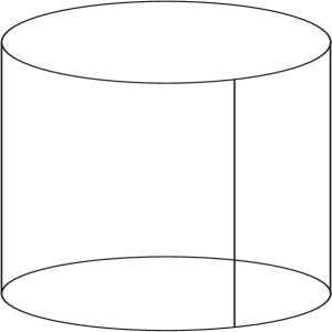
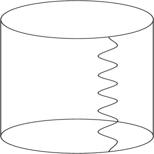
Figure 1: Brane with trivial topology in $M_{3}=M_{2}\times S^{1}$. The ground state of the brane is represented on the left. On the right we plot an excited stated.

As shown in [14], if the brane ground state is $Y^{m}(x)=Y^{m}_{0}$, the presence of the brane will break spontaneously all the $B$ isometries, except those that leave the point $Y_{0}$ unchanged. In other words the group $G(B)$ is spontaneously broken down to the isotropy group $H(Y_{0})$ of the point $Y_{0}$. We will denote $\xi_{\alpha}$ the Killing fields associated with the broken generators of the group $G(B)$. The excitations of the brane along $\xi_{\alpha}$ correspond to the zero modes and they are parametrized by the branon fields $\pi^{\alpha}(x)$ which can be understood as coordinates on the coset manifold $K=G(B)/H$. Thus, for a position-independent ground state $Y^{m}_{0}$, the action of an element of $G(B)$ on $B$ will map $Y_{0}$ into some other point with coordinates:

$$Y^{m}(x)=Y^{m}(Y_{0},\pi^{\alpha}(x))=Y^{m}_{0}+\frac{1}{kf^{2}}\xi^{m}_{\alpha}(Y_{0})\pi^{\alpha}(x)+{\cal O}(\pi^{2}),$$ (6)

where we have set the appropriate normalization of the branon fields and Killing fields with $k^{2}=16\pi/M_{P}^{2}$. When the $B$ space is homogeneous, the isotropy group does not depend on the particular point we choose, i.e, $H(Y_{0})=H$ and it is possible to prove that $B$ is diffeomorphic to $K=G(B)/H$, i.e. the number of GB equals the dimension of $B$. In that case we can choose the coordinates on $B$ and $K$ so that

$$\pi^{\alpha}=\frac{v}{R_{B}}\delta_{m}^{\alpha}y^{m}=f^{2}\delta_{m}^{\alpha}y^{m},$$ (7)

or

$$Y^{m}=\frac{1}{f^{2}}\delta_{\alpha}^{m}\pi^{\alpha},$$ (8)

where

$$v=f^{2}R_{B},$$ (9)

is the typical size of $K$ in energy units (note that the coordinates on $K$ must be scalar fields) and $R_{B}$ is the $B$ typical scale in length units. However, in the general case, $B$ is not homogeneous and the number of GB will be smaller than the dimension of $B$. Notice that since $\pi^{\alpha}$ are properly normalized scalar fields, the $Y^{m}$ coordinates in (8) must be normal and geodesic in a neighborhood of $Y^{m}_{0}$ and, in particular, they cannot be angular coordinates.

According to the previous discussion, we can write the induced metric in terms of branon fields, thus using (6) we get:

$$g_{\mu\nu}=\tilde{g}_{\mu\nu}-\frac{1}{f^{4}}h_{\alpha\beta}(\pi)\partial_{\mu}\pi^{\alpha}\partial_{\nu}\pi^{\beta}$$ (10)

where $h_{\alpha\beta}(\pi)$ is defined as

$$h_{\alpha\beta}(\pi)=f^{4}\tilde{g}^{\prime}_{mn}(Y(\pi))\frac{\partial Y^{m}}{\partial\pi^{\alpha}}\frac{\partial Y^{n}}{\partial\pi^{\beta}}.$$ (11)

Using these results, it is also possible to obtain the expansion of the effective action in (5) in terms of branons (for a detailed discussion see the Appendix).

3 Ground state of the brane and branon masses

In the previous section we assumed that the $G(M_{D})$ symmetry is exact, which implies that the branon fields are massless. However, in a real situation, such symmetry will be only approximately realized. In this case, we will expect the branons to acquire a mass that will measure the breaking of the $G(M_{D})$ symmetry. In order to study these effects and how the symmetry breaking affects the brane ground state, we will relax the conditions imposed in the previous section and let $\tilde{g}_{\mu\nu}$ depend, not only on the $x$ coordinates, but also on the $y$ coordinates. We can consider for simplicity the lowest-order action, given by:

$$S_{eff}^{(0)}[\pi] = \int_{M_{4}}d^{4}x{\mathcal{L}}^{(0)}=-f^{4}\int_{M_{4}}d^{4}x\sqrt{\tilde{g}(x,Y(x))}.$$ (12)

This action has an extremum if

$$\delta S_{eff}^{(0)}[\pi]=0\Rightarrow\delta\sqrt{\tilde{g}}=\frac{1}{2}\sqrt{\tilde{g}}\tilde{g}^{\mu\nu}\delta\tilde{g}_{\mu\nu}=0\Rightarrow\tilde{g}^{\mu\nu}\partial_{m}\tilde{g}_{\mu\nu}=0,\forall y^{m}.$$ (13)

This is a set of equations whose solution $Y^{m}_{0}(x)$ determines the shape of the brane in its ground state for a given background metric $\tilde{g}_{\mu\nu}$. In addition, the condition for the energy to be a minimum requires:

$$\left.\frac{\delta^{2}{\mathcal{L}}^{(0)}}{\delta Y^{m}\delta Y^{n}}\right|_{Y=Y_{0}} = \frac{-f^{4}}{4}\sqrt{\tilde{g}}\tilde{g}^{\mu\nu}(\partial_{n}\partial_{m}\tilde{g}_{\mu\nu}-2\tilde{g}^{\rho\sigma}\partial_{n}\tilde{g}_{\nu\sigma}\partial_{m}\tilde{g}_{\mu\rho})<0.$$ (14)

i.e. the eigenvalues of the above matrix should be negative. This implies that the static action should have a maximum (Dashen condition). If we only focus on the degrees of freedom associated to the branons, the previous conditions take the form:

$$\frac{\delta{\mathcal{L}}^{(0)}}{\delta\pi^{\alpha}} = \frac{-f^{2}}{2k}\sqrt{\tilde{g}}\tilde{g}^{\mu\nu}\partial_{m}\tilde{g}_{\mu\nu}\xi^{m}_{\alpha}=0,$$ (15)

$$\frac{\delta^{2}{\mathcal{L}}^{(0)}}{\delta\pi^{\alpha}\delta\pi^{\beta}} = -\frac{1}{4k^{2}}\sqrt{\tilde{g}}\tilde{g}^{\mu\nu}(\partial_{n}\partial_{m}\tilde{g}_{\mu\nu}-2\tilde{g}^{\rho\sigma}\partial_{n}\tilde{g}_{\nu\sigma}\partial_{m}\tilde{g}_{\mu\rho})\xi^{m}_{\alpha}\xi^{n}_{\beta}<0.$$

In order to obtain the explicit expression for the branon mass matrix, let us consider the following simple case:

$$G_{MN} = \left(\begin{array}[]{cccc}\tilde{g}_{\mu\nu}(x,y)&0\\ 0&-\tilde{g}^{\prime}_{mn}(y)\end{array}\right),$$ (18)

where again $\tilde{g}_{\mu\nu}(x,Y_{0})$ corresponds to the ground state metric in the symmetric case. Expanding this metric around $y^{m}=Y^{m}_{0}$ in terms of the $\pi^{\alpha}$ fields and taking into account the conditions for the ground state of the brane (15), the effective action is then given by

$$S_{B} = -f^{4}\int_{M_{4}}d^{4}x\sqrt{\tilde{g}}$$ (19)

$$+ \frac{1}{2}\int_{M_{4}}d^{4}x\sqrt{\tilde{g}}(\tilde{g}^{\mu\nu}h_{\alpha\beta}(\pi)\partial_{\mu}\pi^{\alpha}\partial_{\nu}\pi^{\beta}-M^{2}_{\alpha\beta}\pi^{\alpha}\pi^{\beta})+...$$

where $\tilde{g}^{\mu\nu}$ in the previous equation denotes $\tilde{g}^{\mu\nu}(x,Y_{0})$ and the mass matrix can be written as

$$M^{2}_{\alpha\beta}=\frac{1}{2}\tilde{g}^{\mu\nu}(\partial_{n}\partial_{m}\tilde{g}_{\mu\nu}-2\tilde{g}^{\rho\sigma}\partial_{n}\tilde{g}_{\nu\sigma}\partial_{m}\tilde{g}_{\mu\rho})\frac{\xi^{m}_{\alpha}\xi^{n}_{\beta}}{k^{2}}>0,$$ (20)

which must be positive definite, otherwise the brane ground state would not be stable. As an example, and for further reference let us consider a background metric given by:

$$\tilde{g}_{\mu\nu}=(1+\sigma(y^{2}))\eta_{\mu\nu},$$ (21)

where $y_{m}$ are normal geodesic coordinates on $B=S^{3}$, $y^{2}=\sum_{m}y_{m}^{2}$ and the function $\sigma(y^{2})$ reaches its minimum value at $y=0$ with $\sigma(0)=0$. The ground state conditions imply:

$$\partial_{m}\sigma\frac{\xi^{m}_{\alpha}}{k}=0$$ (22)

and

$$M^{2}_{\alpha\beta}=2\partial_{n}\partial_{m}\sigma\frac{\xi^{m}_{\alpha}\xi^{n}_{\beta}}{k^{2}}>0.$$ (23)

Since in this case we have $\xi^{m}_{\alpha}=k\delta^{m}_{\alpha}$ we obtain a diagonal mass matrix with all the branons having the same mass $m^{2}=4\sigma^{\prime}(0)$ and then:

$$M^{2}_{\alpha\beta}=m^{2}\delta_{mn}\frac{\xi^{m}_{\alpha}\xi^{n}_{\beta}}{k^{2}}=m^{2}\delta_{\alpha\beta}.$$ (24)

4 Brane-skyrmions

The branon fields introduced in the previous sections describe small oscillations of the brane around its ground state. Thus there is some similarity with the well-known chiral lagrangian approach in which a non-linear sigma model (NLSM) is used to describe the low-energy pion dynamics. Apart from pions, the NLSM can also be used to describe other non-trivial states in the hadron spectrum such as baryons. For that purpose, the non-trivial topological structure of the coset space $K$ plays a fundamental role. In fact, baryons can be identified with certain topologically non-trivial maps between the (compactified) space $S^{3}$ and the coset manifold $K$ known as Skyrmions.

Let us then consider static branon field configurations with finite energy, which accordingly vanish at the spatial infinity. Thus, we can compactify the spatial dimensions to $S^{3}$ and the static configurations will be mappings: $\pi^{\alpha}:S^{3}\rightarrow K$. Therefore, these mappings can be classified according to the third homotopy group of $K$, i.e. $\pi_{3}(K)$. As a consequence, mappings belonging to different non-trivial homotopy classes cannot be deformed in a continuous fashion from one to the other. This implies that such configurations cannot evolve in time classically into the trivial vacuum $\pi=0$ and therefore they are stable states. For the sake of simplicity we will first consider the case in which we have $N=3$ extra dimensions with $B=S^{3}$. In this case, since $B$ is an homogeneous space, we have $K\sim B=S^{3}\sim SU(2)$, i.e the coset manifold is also a 3-sphere. Thus, we will have $\pi_{3}(S^{3})=\bf{Z}$ and the mappings can be classified by an integer number, usually referred to as the winding number $n_{W}$. We will also assume in the following, that the background metric is flat, i.e, $\tilde{g}_{\mu\nu}=\eta_{\mu\nu}$.

For static configurations the brane-skyrmion mass can be obtained directly from the effective lagrangian as:

$$M[\pi]=-\int d^{3}x{\cal L}_{eff}.$$ (25)

In general this expression will be divergent because of the volume contribution coming from the lowest order term $S^{(0)}_{eff}[\pi]$ which reflects the fact that the brane has infinite extension with finite tension. Therefore, in order to obtain a finite skyrmion mass, we will subtract the vacuum energy $M[0]$, i.e.:

$$M_{S}[\pi]=M[\pi]-M[0]=f^{4}\int_{M_{3}}d^{3}x\sqrt{g}-\lambda f^{2}\int_{M_{3}}d^{3}x\sqrt{g}R-M[0].$$ (26)

In other words we are defining the mass of the brane-skyrmion as the mass of the brane with the topological defect minus the mass of the brane in its ground state without topological defect.

In order to simplify the calculations we will introduce spherical coordinates on both spaces, $M_{4}$ and $K$. In $M_{4}$ we denote the coordinates $\{t,r,\theta,\varphi\}$ with $\phi\in[0,2\pi)$, $\theta\in[0,\pi]$ and $r\in[0,\infty)$. In these coordinates the background metric is written as:

$$\tilde{g}_{\mu\nu}=\left(\begin{array}[]{cccc}1&\\ &-1&\\ &&-r^{2}&\\ &&&-r^{2}\sin^{2}(\theta)\end{array}\right).$$ (31)

On the coset manifold $K$, the spherical coordinates are denoted $\{\chi_{K},\theta_{K},\phi_{K}\}$ with $\phi_{K}\in[0,2\pi)$, $\theta_{K}\in[0,\pi]$ and $\chi_{K}\in[0,\pi]$. These coordinates are related to the physical branon fields (local normal geodesic coordinates on $K$) by:

$$\pi_{1} = v\sin\chi_{K}\sin\theta_{K}\cos\phi_{K},$$

$$\pi_{2} = v\sin\chi_{K}\sin\theta_{K}\sin\phi_{K},$$ (32)

$$\pi_{3} = v\sin\chi_{K}\cos\theta_{K}.$$

The coset metric in spherical coordinates is written as

$$h_{\alpha\beta}=\left(\begin{array}[]{ccc}v^{2}&\\ &v^{2}\sin^{2}(\chi_{K})&\\ &&v^{2}\sin^{2}(\chi_{K})\sin^{2}(\theta_{K})\end{array}\right).$$ (36)

In spherical coordinates, the brane-skyrmion with winding number $n_{W}$ is given by the non-trivial mapping $\pi^{\alpha}:S^{3}\longrightarrow S^{3}$ defined from:

$$\phi_{K} = \phi,$$

$$\theta_{K} = \theta,$$

$$\chi_{K} = F(r),$$ (37)

with boundary conditions $F(0)=n_{W}\pi$ and $F(\infty)=0$. This map is usually referred to as the hedgehog ansatz. In Fig. 2 we plot on the right a Skyrmion-like 1-brane configuration in $M_{3}=M_{2}\times S^{1}$. In this particular dimension the brane-skyrmion is not stable (as shown below), but still it is useful for illustrative purposes.

                 

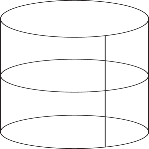
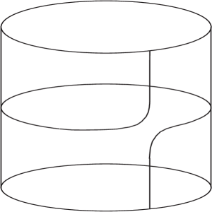
Figure 2: Brane configurations with $n_{W}=1$ in $M_{3}=M_{2}\times S^{1}$. On the right we plot a non-zero size Skyrmion. On the left a zero-size 1-brane-skyrmion is shown. It has the same mass and shape as the state built out of a wrapped soliton and a topologically trivial (world) brane. However the topology is not the same (see section 9).

Notice once again that the spherical coordinates we have introduced on $K$ cannot be directly understood as branon fields, although, thanks to the reparametrization invariance of the action, they are perfectly valid for performing the calculations.

In order to calculate the brane-skyrmion mass from (26), we need explicit expressions for the induced metric determinant and the scalar curvature. In these coordinates the induced metric on the brane is given by the diagonal matrix

$$g_{\mu\nu}=\left(\begin{array}[]{cccc}1\vspace{.1cm}&\\ &-\left(1+\frac{v^{2}}{f^{4}}(F^{\prime}(r))^{2}\right)\vspace{.1cm}&\\ &&-\left(r^{2}+\frac{v^{2}}{f^{4}}\sin^{2}(F(r))\right)\vspace{.1cm}&\\ &&&-\left(r^{2}+\frac{v^{2}}{f^{4}}\sin^{2}(F(r))\right)\sin^{2}(\theta)\end{array}\right),$$ (42)

and the corresponding square root of the determinant can be easily found to be:

$$\sqrt{g}=\sqrt{1+\frac{v^{2}}{f^{4}}(F^{\prime}(r))^{2}}\left(r^{2}+\frac{v^{2}}{f^{4}}\sin^{2}(F(r))\right)\sin(\theta).$$ (43)

The induced scalar curvature can be obtained in a simple way by introducing the isotropic coordinates $\{t,\rho,\theta,\varphi\}$ where $\rho$ is defined as

$$\rho^{2}\equiv r^{2}+\frac{v^{2}}{f^{4}}\sin^{2}(F(r)).$$ (44)

The metric in these new coordinates is written in the isotropic canonical form:

$$g_{\mu\nu}=\left(\begin{array}[]{cccc}1&\\ &-A(r)&\\ &&-\rho^{2}&\\ &&&-\rho^{2}\sin^{2}(\theta)\end{array}\right),$$ (49)

where

$$A(r)=\frac{1+\frac{v^{2}}{f^{4}}(F^{\prime}(r))^{2}}{\rho^{\prime 2}},$$ (50)

and ^′ denotes $r$ derivative. The scalar curvature for this metric turns out to be:

$$R=-\frac{2}{\rho^{2}}\left(1-\frac{1}{A(r)}\right)-\frac{2A^{\prime}(r)}{A^{2}(r)\rho\rho^{\prime}}.$$ (51)

Thus we can write $M_{S}$ as a functional of $F(r)$. The actual mass of the brane-skyrmion with winding number $n_{W}$ will be obtained by minimizing the functional $M_{S}[F]$ (26) in the space of functions $F(r)$ with the appropriate boundary conditions. This problem is in general rather complicated, but we can obtain an upper bound to the mass by using a family of functions parametrized by a single parameter, and minimizing with respect to that parameter. In particular, it is very useful to work with the Atiyah-Manton ansatz [20]:

$$F(r)=n_{W}\pi\left(1-\frac{1}{\sqrt{1+L^{2}/r^{2}}}\right).$$ (52)

By minimizing the brane-skyrmion mass with respect to $L$ we will get: $M_{S}\equiv min_{L}\;M_{S}(L)\equiv M_{S}(L_{m})$ for different values of the parameter $\lambda$. Thus:

• For $\lambda=0$ and using the ansatz above for $n_{W}=1$ we find that $M_{S}(L)$ is minimized for $L_{m}=0$. The corresponding mass is given by

  $$M_{S}=2\pi^{2}f^{4}R_{B}^{3},$$ (53)

  i.e. the brane-skyrmion describes a pointlike particle with a finite mass given by the volume of the extra dimensions times the brane tension $f^{4}$. It can be shown (see next section) that this result is general, i.e. it is valid for any parametrization of the $F(r)$ function and not only for the Atiyah-Manton one.

• For $\lambda>0$, we find that $M_{S}(L)$ is minimized for some $L_{m}>0$ (non-zero size brane-skyrmion). In this case, assuming that the contribution from the curvature term never becomes negative, it is possible to obtain the following lower bound on the mass $M_{S}>M_{S}(\lambda=0)=2\pi^{2}f^{4}R_{B}^{3}$. An upper bound can be obtained by evaluating $M_{S}$ in the limit $L=0$, simply assuming that this limit is well defined so that we can commute the limit with the integration. Thus

  $$M_{S}<M_{S}(L=0)=2\pi^{2}f^{4}R_{B}^{3}\left(1+6\frac{\lambda}{R_{B}^{2}f^{2}}\right).$$ (54)

  These results are general for any monotonic parametrization and, in particular, we have checked numerically that they hold for the Atiyah-Manton case.

• Finally, for $\lambda<0$, we find again that the minimum $M_{S}$ corresponds to zero size brane-Skyrmion and the corresponding mass is

  $$M_{S}=2\pi^{2}f^{4}R_{B}^{3}\left(1+6\frac{\lambda}{R_{B}^{2}f^{2}}\right).$$ (55)

  When $\lambda<-R_{B}^{2}f^{2}/6$ the brane-skyrmion mass becomes negative. In this case, using non-monotonic parametrizations, we have obtained that the mass is actually not bounded from below, since the curvature term can be made arbitrarily large. As a consequence only in this last case, the brane-skyrmion becomes unstable. These results are summarized in Table.1

$\lambda$	Size	Mass
$\lambda=0$	$L_{m}=0$	$M_{S}=2\pi^{2}f^{4}R_{B}^{3}$
$\lambda>0$	$L_{m}>0$	$2\pi^{2}f^{4}R_{B}^{3}<M_{S}<2\pi^{2}f^{4}R_{B}^{3}(1+6\frac{\lambda}{R_{B}^{2}f^{2}})$
$-R_{B}^{2}f^{2}/6<\lambda<0$	$L_{m}=0$	$M_{S}=2\pi^{2}f^{4}R_{B}^{3}(1+6\frac{\lambda}{R_{B}^{2}f^{2}})$
$\lambda<-R_{B}^{2}f^{2}/6$	$L_{m}=0$	$M_{S}\rightarrow-\infty$

Table 1: Values of the size $L_{m}$ and mass $M_{S}$ for the brane-skyrmion with $n_{W}=1$ for different values of the $\lambda$ parameter

In Fig.3 we show the brane-skyrmion mass as a function of $\lambda$ and $L$. We see that the minimum is displaced from $L=0$ when $\lambda>0$.

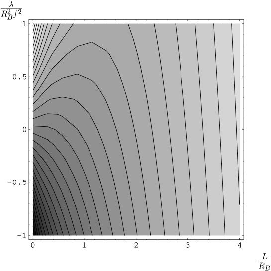
Figure 3: Contour plot of the brane-skyrmion mass as a function of $\lambda/(R_{B}^{2}f^{2})$ and $L/R_{B}$.

Notice that these results differ a lot from those obtained in the usual $SU(2)$ Skyrme model in QCD chiral dynamics [12, 19]. That model is based on a fourth-order lagrangian and only within a certain range of the parameters $M$ and $N$ of the two independent four-derivative terms, the Skyrmion can be made stable. In our case, the lagrangian contains an infinite number of terms, which are responsible for the brane-skyrmion stability. In fact, truncating the series and keeping only up to fourth order terms, one obtains in our case:

$$S_{eff}^{(2,4)}[\pi] = \frac{1}{2}\int_{M_{4}}d^{4}x\sqrt{\tilde{g}}h_{\alpha\beta}\partial_{\mu}\pi^{\alpha}\partial^{\mu}\pi^{\beta}$$ (56)

$$+ \frac{1}{4v^{4}}\int_{M_{4}}d^{4}x\sqrt{\tilde{g}}h_{\alpha\beta}h_{\gamma\delta}(M\partial_{\mu}\pi^{\alpha}\partial^{\mu}\pi^{\beta}\partial_{\nu}\pi^{\gamma}\partial^{\nu}\pi^{\delta}$$

$$+ N\partial_{\mu}\pi^{\alpha}\partial^{\nu}\pi^{\beta}\partial_{\nu}\pi^{\gamma}\partial^{\mu}\pi^{\delta}),$$

where we have assumed $\tilde{g}_{\mu\nu}=\eta_{\mu\nu}$. The corresponding $M$ and $N$ parameters in the chiral lagrangian are then given by:

$$M=\frac{-f^{4}R_{B}^{4}}{32},\;\;N=\frac{f^{4}R_{B}^{4}}{16}.$$ (57)

This implies that the standard $e^{2}$ and $\gamma$ Skyrme-model parameters are

$$e^{2}=\frac{1}{16N}=\frac{1}{f^{4}R_{B}^{4}}>0,\;\;\gamma=\frac{1}{2}\left(1+\frac{M}{N}\right)=\frac{1}{4}>0,$$ (58)

which means that the Skyrmion would not be stable if one had considered the truncated fourth-order lagrangian only. However, for the full lagrangian (with $\lambda>-R_{B}^{2}f^{2}/6$) we have seen before that the brane-skyrmion is stable. This shows that the infinite number of higher-order terms are responsible for its stability. This of course could also be the case in chiral dynamics. In this case, it is also possible to compute the $M$ and $N$ parameters in the framework of large $N_{c}$ Quantum Cromodynamics (QCD) (for a review see [17])

$$M=\frac{N_{c}}{192\pi^{2}},\;\;N=\frac{-N_{c}}{384\pi^{2}},$$ (59)

which implies $M/N=-2$. It is quite amazing to realize that this is exactly the same relation found in the branon dynamics. In particular for:

$$N_{c}=12\pi^{2}f^{4}R_{B}^{4}$$ (60)

we have the same answer in the two models, provided we identify $v=F_{\pi}$, $F_{\pi}$ being the pion decay constant. Thus for $N_{c}=3$ one can set $R_{B}^{2}=1/(2\pi f^{2})$ in such a way that the branon dynamics could reproduce the correct low-energy pion scattering and give rise to a stable nucleon. We really do not have any particular reason to understand why this simple brane model works so well apart from having the same symmetry breaking pattern as the low-energy chiral dynamics.

5 Numerical results

As we saw in the previous section, if $\lambda>0$, the brane-skyrmion size is different from zero and its mass cannot be evaluated analytically although some bounds can be obtained. For this reason, it is very interesting to obtain the behaviour of the brane-skyrmion size and mass as a function of $\lambda$, at least numerically. As shown in the previous section, the contribution of the curvature term to the brane-skyrmion mass depends on $\lambda/(R_{B}^{2}f^{2})$. Assuming that such contribution is small we have performed a numerical analysis in the case $B=S^{3}$ using the Atiyah-Manton parametrization. For the brane-skyrmion size in the mentioned limit we find the following behaviour:

$$\frac{L_{m}}{R_{B}}=\left\{\begin{array}[]{cc}0;&\lambda\leq 0\\ &\\ a\left(\frac{\lambda}{R_{B}^{2}f^{2}}\right)^{\alpha};&\lambda>0\end{array}\right.,$$ (64)

where the value of the $a$ and $\alpha$ parameters are given in Table.2. In Figure 4, we show this non-analytic behavior for the brane-skyrmion size with $n_{W}=1$.

Figure 4: Behaviour of the brane-skyrmion size with $n_{W}=1$ when $\lambda/R_{B}^{2}f^{2}$ is small.

The fact that the brane-skyrmion acquires a non-zero size implies that its mass depends on $\lambda$ in a non-trivial way. The numerical calculation shows that the behaviour of the brane-skyrmion mass in the mentioned limit is of the form:

$$\frac{M_{S}}{4\pi f^{4}R_{B}^{3}}=\left\{\begin{array}[]{cc}\frac{|n_{W}|\pi}{2}+3|n_{W}|\left(\frac{\lambda}{R_{B}^{2}f^{2}}\right);&\lambda\leq 0\\ &\\ \frac{|n_{W}|\pi}{2}+3|n_{W}|\left(\frac{\lambda}{R_{B}^{2}f^{2}}\right)-b\left(\frac{\lambda}{R_{B}^{2}f^{2}}\right)^{\beta};&\lambda>0\end{array}\right.,$$ (68)

where the value of the parameters $b$ and $\beta$ is shown in Table.2 for different winding numbers $n_{W}$. The non-analytic behaviour of the derivative with respect to $\lambda$ is plotted in Fig.5 for $n_{W}=1$. The numerical calculation for the Atiyah-Manton ansatz shows that the constants $a$ and $b$ depend on $n_{W}$ in a non-trivial way, whereas the exponents $\alpha$ and $\beta$ do not.

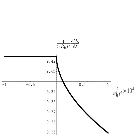
Figure 5: Behaviour of the derivative with respect to $\lambda$ of the brane-skyrmion mass with $n_{W}=1$ for small $\lambda/(R_{B}^{2}f^{2})$.

An interesting conclusion that can be obtained from these results is that the interaction between two classical brane-skyrmions with topological number $n_{W}=1$ is repulsive when their sizes are non zero, whereas they do not interact if their sizes are exactly zero. The reason is that one could understand a $n_{W}=2$ brane-skyrmion as two $n_{W}=1$ brane-skyrmions located at the same point. The energy of the $n_{W}=2$ brane-skyrmion is bigger than the energy of two brane-skyrmions with $n_{W}=1$ if their sizes are non zero, whereas it is the same if their sizes are exactly zero.

Topological	$\alpha$	$\beta$	$a$	$b$
charge $n_{W}$
1	0.81	1.54	0.97	7.1
2	0.81	1.54	0.59	6.5
3	0.81	1.54	0.44	6.2

Table 2: Values of the constants $a$, $b$, $\alpha$ and $\beta$ for different topological numbers $n_{W}$ in the Atiyah-Manton ansatz.

It is important to notice that these numerical results have been obtained with the hedgehog ansatz and the Atiyah-Manton parametrization and therefore they are only estimations of the true mass and size. In fact, it is known from the standard Skyrme model for baryons that the hedgehog ansatz is not appropriate for the description of the deuteron, corresponding to a $n_{W}=2$ Skyrmion since there is other toroidal-like configuration with less energy in this topological sector.

6 Brane-skyrmions in higher dimensions

In this section we will extend our previous discussion to an arbitrary number $N$ of space and compactified dimensions. We will start from the simplest case with $\lambda=0$. Let us consider the Dirac-Nambu-Goto action for a N-brane:

$$S_{B}=-f^{N+1}\int_{M_{N+1}}dt\;d^{N}x\sqrt{g}.$$ (69)

For simplicity, we will take $\tilde{g}_{\mu\nu}=\eta_{\mu\nu}$ and $K=S^{N}$, so that $M_{D}=M_{N+1}\times S^{N}$ with $D=2N+1$. The generalization of the hedgehog ansatz to $N$ dimensions with winding number $n_{W}$ can be written more easily in angular coordinates as follows:

$$\begin{array}[]{lll}\phi_{K}=\phi&\phi_{K}\in[0,2\pi),&\phi\in[0,2\pi)\\ \theta^{i}_{K}=\theta^{i}&\theta^{i}_{K}\in[0,\pi],&\theta^{i}\in[0,\pi],\;i=1..\;N-2\\ \chi_{K}=F(r)&\chi_{K}\in[0,n_{W}\pi],&r\in[0,\infty),\end{array}$$ (71)

where the $K$ subindex refers to coordinates on the $K$ manifold, the angular coordinates on $M_{N+1}$ do not carry any subindex and the chiral angle function $F(r)$ satisfies the boundary conditions $F(0)=n_{W}\pi$, $F(\infty)=0$. Introducing again $\rho$ as in (44), the induced metric takes the spherically symmetric form:

$$g_{\mu\nu}=\left(\begin{array}[]{ccccccccc}1&\\ &-A(r)&\\ &&-\rho^{2}&\\ &&&-\rho^{2}\sin^{2}\theta_{N-2}&\\ &&&&-\rho^{2}\sin^{2}\theta_{N-2}\sin^{2}\theta_{N-3}&\\ &&&&&.&\\ &&&&&&.&\\ &&&&&&&.&\\ &&&&&&&&-\rho^{2}\sin^{2}\theta_{N-2}...\sin^{2}\theta_{1}\end{array}\right)$$ (81)

where $A(r)$ is given in equation (50). For static configurations, the Dirac-Nambu-Goto action (69) provides the mass functional:

$$M_{S} = f^{N+1}\int d^{N}x\left(\det\left(g_{\mu\nu}\right)^{1/2}-\det(\eta_{\mu\nu})^{1/2}\right)$$

$$= f^{N+1}\Omega_{N}\int dr\left(\left[r^{2}+\frac{v^{2}}{f^{4}}\sin^{2}F(r)\right]^{\frac{N-1}{2}}\left[1+\frac{v^{2}}{f^{4}}F^{\prime}(r)^{2}\right]^{\frac{1}{2}}-r^{N-1}\right),$$

where the total solid angle is given by:

$$\Omega_{N}=\frac{2\pi^{N/2}}{\Gamma(N/2)}.$$ (83)

For $N\geq 2$ it is possible to obtain a non-trivial bound for $M_{S}$. $N=1$ is a special case and will be studied later on. Let us start from the inequality:

$$(a+b)^{\frac{N-1}{2}}\geq(a^{N-1}+b^{N-1})^{1/2},$$ (84)

which is valid for $N\geq 2$ and $a,b>0$. We will also use:

$$(a+b)^{1/2}(c+d)^{1/2}\geq ac+bd,$$ (85)

again for $a,b,c,d>0$. From (LABEL:Nmass) we obtain:

$$M_{S}\geq f^{N+1}\Omega_{N}\int dr\left(\frac{v}{f^{2}}\right)^{N}|\sin^{N-1}(F(r))||F^{\prime}(r)|.$$ (86)

Since $v=R_{B}f^{2}$ we have:

$$M_{S} \geq f^{N+1}R_{B}^{N}\Omega_{N}\int dr|\sin^{N-1}(F(r))||F^{\prime}(r)|$$ (87)

$$= f^{N+1}R_{B}^{N}\Omega_{N}\int_{0}^{n_{W}\pi}du|\sin^{N-1}(u)|,$$

where in the last step, we have defined $u=F(r)$, assuming that $F(r)$ is a monotonic function.

The total volume of the $S^{N}$ sphere with radius $R_{B}$ is given by:

$$V_{N}(R_{B})=\frac{2\pi^{\frac{N+1}{2}}}{\Gamma\left(\frac{N+1}{2}\right)}R_{B}^{N}=R_{B}^{N}\Omega_{N+1}.$$ (88)

Accordingly, we can write the bound on the mass as:

$$M_{S}\geq M_{Sm}\equiv|n_{W}|f^{N+1}R_{B}^{N}\Omega_{N+1}=|n_{W}|f^{N+1}V_{N}(R_{B}).$$ (89)

This is a lower bound for $N\geq 2$. On the other hand, we can write the chiral angle as $F(r)=\bar{F}(r/L)=\bar{F}(\bar{r})$ with $\bar{r}=r/L$, $L$ being the typical brane-skyrmion size. Thus, the mass functional can be written as:

$$M_{S} = f^{N+1}\Omega_{N}L\int d\bar{r}\left(\left[L^{2}\bar{r}^{2}+R_{B}^{2}\sin^{2}\bar{F}(\bar{r})\right]^{\frac{N-1}{2}}\left[1+\frac{R_{B}^{2}}{L^{2}}\left(\frac{d\bar{F}}{d\bar{r}}\right)^{2}\right]^{\frac{1}{2}}\right.$$ (90)

$$- \left.(L\bar{r})^{N-1}\right).$$

Taking the limit $L\rightarrow 0$ in the above integral, we find that it is well defined and $M_{S}\rightarrow M_{Sm}$, i.e., zero size brane-skyrmions saturate the bound. Therefore the Skyrmion mass is $M_{S}=M_{Sm}$ and the Skyrmion is pointlike ($L_{m}=0$) for $N\geq 2$.

In the case $N=1$, the inequalities above cannot be used and the only bound is the trivial one, i.e. $M_{S}\geq 0$. It is possible to show from (90) that in this case, the bound is saturated in the opposite limit $L\rightarrow\infty$. Accordingly, 1-brane-Skyrmions in one extra dimension would be massless and non-localized.

Let us consider now the effect of the brane-induced curvature $R$ term, i.e. $\lambda\neq 0$. This curvature is given by

$$R=-(N-1)\left[\frac{(N-2)}{\rho^{2}}\left(1-\frac{1}{A(r)}\right)+\frac{A^{\prime}(r)}{A^{2}(r)\rho\rho^{\prime}}\right].$$ (91)

Following the same steps as in the $N=3$ case, we obtain the following results. For $\lambda\in(0,\infty)$ and $n_{W}=1$ we have $L_{m}>0$ and the mass of the brane-skyrmion is bounded in the range

$$\frac{2\pi^{\frac{N+1}{2}}}{\Gamma(\frac{N+1}{2})}f^{N+1}R_{B}^{N}<M_{S}<2\frac{2\pi^{\frac{N+1}{2}}}{\Gamma(\frac{N+1}{2})}f^{N+1}R_{B}^{N}\left(1+N(N-1)\frac{\lambda}{R_{B}^{2}f^{2}}\right).$$ (92)

For $\lambda\leq 0$ the brane-skyrmion colapses i.e. $L_{m}=0$ and the mass of the brane-skyrmion can be computed as in the $N=3$ case to find:

$$M_{S}=2\frac{2\pi^{\frac{N+1}{2}}}{\Gamma(\frac{N+1}{2})}f^{N+1}R_{B}^{N}\left(1+N(N-1)\frac{\lambda}{R_{B}^{2}f^{2}}\right).$$ (93)

Finally, for $\lambda<-R_{B}^{2}f^{2}/N(N-1)$ the brane-skyrmion mass is negative and not bounded from below.

The previous generalization is appropriate for $N\geq 3$. For the particular case $N=2$ it is possible to show that the curvature integrates to zero. This is because in this case we have

$$R=-\frac{A^{\prime}(r)}{A^{2}(r)\rho\rho^{\prime}}$$ (94)

and

$$g=A(r)\rho^{2}(\rho^{\prime})^{2}.$$ (95)

Then, taking into account that $1/\sqrt{A}$ vanishes whenever $\rho^{\prime}$ is zero

$$\int_{M_{2}}d^{2}x\sqrt{g}R=-\int^{\infty}_{0}dr\int^{2\pi}_{0}d\theta\frac{A^{\prime}}{A^{3/2}}\mbox{sign}(\rho^{\prime})=\left.\frac{\pi}{\sqrt{A}}\right|^{\infty}_{0}=0.$$ (96)

Therefore, we can conclude that the 2-brane-skyrmion is always point like. This can be understood by realizing that in two dimensions the scalar curvature integral is related to the Euler number of the surface, which is a topological invariant and therefore size independent, i.e., unable to give rise to a definite size for the brane-skyrmion.

7 Interaction Lagrangian and fermionic quantization

In this section we will study the interaction between the brane-skyrmions and the branons. For simplicity we will consider only the case $M_{7}=M_{4}\times S^{3}$ with $\tilde{g}_{\mu\nu}=\eta_{\mu\nu}$ so that $K\simeq SU(2)$. Then we can follow the well-known steps for quantization of the standard chiral-dynamics Skyrmion [19]. It is possible to split the isometry group $G$ as $G=SU(2)_{L}\times SU(2)_{R}$ and $H$ corresponds to the isospin group $SU(2)_{L+R}$. The parametrization of the coset is usually done in terms of an $SU(2)$ matrix $U(x)$ and the Skyrmion is written as

$$U(x) = \exp(iF(r)\hat{x}^{a}\tau^{a})=\cos F(r)+i\tau^{a}\hat{x}^{a}\sin F(r)$$ (97)

$$= \pm\sqrt{1-\frac{\pi^{2}}{v^{2}}}+i\tau^{a}\hat{x}^{a}\sin F(r),$$

where $\tau^{a}$ are the $SU(2)$ generators. From this expression we can identify the Goldstone bosons fields $\pi^{\alpha}=v\sin F(r)\hat{x}^{\alpha}$. The quantization of the isorotations of the Skyrmion solution (which correspond to rotations in the compactified space $B=S^{3}$ in our case) requires the well-known relation $J=I$ where $J$ and $I$ are the spin and the isospin indices. In principle the allowed values of $J$ are $J=0,1/2,1,3/2,...$. As explained by Witten [13], fermionic quantization is possible because of the Wess-Zumino-Witten (WZW) term $k\Gamma$ with $k$ integer, which can be added to the Goldstone boson effective action. For $k$ even the Skyrmion is a boson, but for $k$ odd it is a fermion. For the $SU(2)$ case, the functional $\Gamma$ has no dynamics and becomes a topological invariant related to the homotopy group $\pi_{4}(SU(2))=\bf{Z}_{2}$. Note that for a suitable compactification of the space-time this is the relevant group for the Goldstone boson map. A map belonging to the non-trivial class could, for example, describe the creation of a Skyrmion-antiskyrmion pair followed by a $2\pi$ rotation of the Skyrmion and finally a Skyrmion-antiskyrmion annihilation. In the fermionic case this field configuration must be weighted with a $-1$ in the Feynman path integral. For an adiabatic $2\pi$ rotation of the Skyrmion around some axis, the WZW term contributes $k\pi$ to the action and $(-)^{k}$ to the amplitude which can be understood as an $exp(i2\pi J)$ factor. Therefore both possibilities, bosonic and fermionic quantization of the Skyrmion, are open. In principle this result can also be extended to the more general case of $S^{N}$ brane-skyrmions considered in the last section where $M_{D}=M_{N+1}\times S^{N}$ with $D=2N+1$ since $\pi_{N+1}(S^{N})=\bf{Z}_{2}$ for $N\geq 3$.

In order to study the low-energy interactions of the brane-skyrmions with the branons, we have to obtain the appropriate effective lagrangian. This lagrangian must be $G(B)$ symmetric and the brane-skyrmion should be described in it by a complex field, because of its topological charge. Thus for example this field will be a complex scalar $\Phi$ for $J=0$ or a Dirac spinor $\Psi$ for $J=1/2$. For the scalar case the invariant lagrangian with the lowest number of derivatives can be written as:

$${\cal L}_{s}=\alpha\Phi^{*}\Phi h_{\alpha\beta}(\pi)\partial_{\mu}\pi^{\alpha}\partial^{\mu}\pi^{\beta}.$$ (98)

The coupling $\alpha$ can be obtained from the large distance behaviour of the branon field in the brane-skyrmion configuration. The differential equation for $F(r)$ obtained from the Dirac-Nambu-Goto action in the mentioned limit is the Euler equation:

$$r^{2}F^{\prime\prime}(r)+2rF^{\prime}(r)-2F(r)=0.$$ (99)

The general solution of this equation is:

$$F(r)=Ar+\frac{B}{r^{2}}.$$ (100)

Since we are interested in those solutions in which $F(r)$ goes to zero as $r$ goes to infinity, $A$ has to be identically zero. This means that the general behaviour of $F(r)$ at large distances is

$$F(r)\simeq\frac{B}{r^{2}}.$$ (101)

Therefore in this limit:

$$U(x)=1+i\frac{B}{r^{2}}\hat{x}^{a}\tau^{a}+\dots\simeq 1+iF(r)\hat{x}^{a}\tau^{a}+\dots$$ (102)

Then we have:

$$\pi^{\alpha}\simeq v\frac{B}{r^{2}}\hat{x}^{\alpha},$$ (103)

and in particular for the Atiyah-Manton ansatz with $n_{W}=1$, we get $B=L^{2}\pi/2$. By using the lagrangian ${\cal L}_{s}$ it is also possible to obtain the branon field produced by the brane-skyrmion field $\Phi$ and by comparison with the above results we arrive at [21]

$$\alpha=-\frac{8}{3}\pi^{2}v^{2}B^{2}=-\frac{2}{3}v^{2}\pi^{4}L_{m}^{4}.$$ (104)

From this lagrangian it is possible, for example, to compute the cross sections for producing a brane-skyrmion-antibrane-skyrmion pair from two branons.

The fermionic case can be studied in a similar way [21, 19] although a consistent analysis would be more involved, since it requires the quantization of the rotational modes. This case will be considered elsewhere.

8 Branon mass effects

As shown in Section 3, if the four dimensional metric depends on the extra coordinates, i.e. $\tilde{g}_{\mu\nu}(x,y)$, the branon fields acquire a mass. In order to study the effect of the branon masses on the brane-skyrmion, we will consider the simple case $B=S^{3}$ with $\lambda=0$ and the background metric given in (21). Remember that this metric corresponds to branon fields with equal masses: $m^{2}=4\sigma^{\prime}(0)$. In order to simplify the calculation, we will define a new function $\tilde{\sigma}$ as follows: $\tilde{\sigma}(m^{2}y^{2}/4)=\sigma(y^{2})$. With this definition we have $\tilde{\sigma}(0)=0$ and $\tilde{\sigma}^{\prime}(0)=1$. Using the spherical coordinates on $K$ defined in (32), we can write the background metric as:

$$\tilde{g}_{\mu\nu}=\left(1+\tilde{\sigma}\left(\frac{m^{2}R_{B}^{2}}{4}\sin^{2}(\chi_{K})\right)\right)\eta_{\mu\nu},$$ (105)

where we have used the relation (9). Imposing the Skyrme ansatz in (37), the induced metric on the brane can be written as:

$$ds^{2}=g_{\mu\nu}dx^{\mu}dx^{\nu}=B(r)dt^{2}-A(r)dr^{2}-C(r)(d\theta^{2}+\sin^{2}(\theta)d\phi^{2}),$$ (106)

where:

$$B(r) = 1+\tilde{\sigma}\left(\frac{m^{2}R_{B}^{2}}{4}\sin^{2}(F(r))\right),$$

$$A(r) = B(r)+R_{B}^{2}(F^{\prime}(r))^{2},$$

$$C(r) = r^{2}B(r)+R_{B}^{2}\sin^{2}(F(r)).$$ (107)

Following similar steps to those in the massless case, it is possible to find a lower bound for the brane-skyrmion mass, thus:

$$M_{S} = 4\pi f^{4}\int dr\left(C(r)\sqrt{A(r)B(r)}-r^{2}\right)$$ (108)

$$\geq 4\pi f^{4}\int dr\left(R_{B}^{3}\sin^{2}(F(r))|F^{\prime}(r)|\left[1+\tilde{\sigma}\left(\frac{m^{2}R_{B}^{2}}{4}\sin^{2}(F(r))\right)\right]^{1/2}\right)$$

$$\geq 4\pi|n_{W}|f^{4}R_{B}^{3}\int_{0}^{\pi}du\sin^{2}u\left[1+\tilde{\sigma}\left(\frac{m^{2}R_{B}^{2}}{4}\sin^{2}u\right)\right]^{1/2}.$$

Figure 6: Brane-skyrmion mass $M_{S}$ as a function of the branon mass $m$ in the case $\tilde{\sigma}(\xi)=\xi$ and $n_{W}=1$. The thick continuous line represents the exact dependence; the dashed line, the approximated behavior when $R_{B}m\ll 1$; and the continuous line, the asymptotic behavior when $R_{B}m\gg 1$.

Also in the same way as in the massless case, this lower bound coincides with the zero size brane-skyrmion mass. Therefore, the presence of the branon masses does not affect the brane-skyrmion stability and again we get a pointlike solution. The only difference from the massless case is that the brane-skyrmion mass increases due to the $\tilde{\sigma}$ contribution in the last line of (108).

If the branon mass is small, in $1/R_{B}$ units, we can expand $\tilde{\sigma}(\xi)=\xi+{\cal O}(\xi^{2})$ in (108) and obtain that the dependence of the brane-skyrmion mass on $m$ is quadratic at first order, for any $\tilde{\sigma}$ function:

$$M_{S}=2|n_{W}|\pi^{2}f^{4}R_{B}^{3}\left(1+\frac{3}{16}R_{B}^{2}m^{2}\right).$$ (109)

In the opposite limit, when the contribution of the branon masses to the brane-skyrmion mass is more important than the topological contribution, the brane-skyrmion mass strongly depends on the particular form of the $\tilde{\sigma}$ function. Thus one can find:

$$M_{S}=4\pi|n_{W}|f^{4}R_{B}^{3}\int_{0}^{\pi}du\sin^{2}u\left[\tilde{\sigma}\left(\frac{m^{2}R_{B}^{2}}{4}\sin^{2}u\right)\right]^{1/2}.$$ (110)

Figure 6 shows these behaviours in the simple case $\tilde{\sigma}(\xi)=\xi$.

9 Wrapped states

In this section we are going to study another kind of states which can appear as topological excitations of the branes. These states correspond to brane configurations wrapped around the compactified spaces $B$ which typically will be assumed to be $S^{N}$ for $M_{D}=M_{N+1}\times B$. A given wrapped state is located at some well-defined point of the space $M_{N}$. The possibility of having these wrapped states is related to the homotopy group $\pi_{N}(B)=\bf{Z}$ which is obviously the case for $B=S^{N}$, but also for other spaces. In principle, wrapped states can be present even when there is no world brane, i.e., when we do not have a brane extended along the space $M_{N}$. However, one of the most interesting cases occurs when the wrapped states are located at one point of the world brane and then can be understood as world-brane excitations. Note that as long as the relevant homotopy group is again $\bf{Z}$ we have also antiwrapped states which correspond to negative winding numbers. Thus a world brane can get excited by creating a wrapped-antiwrapped state at some given point. In Fig.7 we show a single wrapped state at rest (left) and branon-excited. On the left of Fig.2 we show a wrapped state (circle) located at one point of the world brane (straight line) for the case $N=1$.

To study in more detail the main properties of these wrapped states we concentrate now on a four-dimensional space-time $M_{4}$ embedded in a $7$-dimensional bulk space that we are assuming to be $M_{7}=M_{4}\times B$ with $M_{4}={\bf R}\times M_{3}$ and $B=S^{3}$. Now, unlike the brane-skyrmion case, here the finite energy requirement does not lead to any compactification of the world space $M_{3}$ because the brane is going to be wrapped around $B$ which is compact. However, for technical reasons it is still useful to compactify $M_{3}$ to $S^{3}$ by adding the spatial infinite point. The wrapped brane produces the spontaneous breaking of the $M_{7}$ isometry group, which we assume to be $G(M_{7})=G({\bf R}\times M_{3}\times S^{3})=G({\bf R}\times S^{3})\times G(M_{3})$ to the $G({\bf R}\times S^{3})\times H^{\prime}$ group where $H^{\prime}$ is the isotropy group of $M_{3}$ which is assumed to be homogeneous. In the previous expressions, ${\bf R}$ corresponds to the time coordinate. Thus, the coset space is defined by $K^{\prime}=G(M_{3})/H^{\prime}$. In the simplest case $M_{3}=S^{3}$ we have $K^{\prime}=SO(4)/SO(3)=S^{3}$ and then $K^{\prime}\sim B\sim S^{3}$. Therefore the low-energy brane excitations can be parametrized as

                 

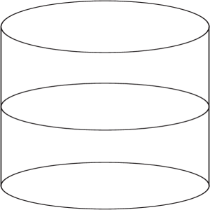
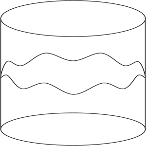
Figure 7: Wrapped brane with topological number 1 in $M_{3}=M_{2}\times S^{1}$. Its ground state is represented on the left and an excited state on the right.

$$\Pi:B \longrightarrow K^{\prime}$$

$$y \longrightarrow \pi(y),$$ (111)

where $y$ are coordinates on $B$ and $\pi$ are coordinates on $K^{\prime}$. On the other hand, as long as the quotient space $K^{\prime}$ and $M_{3}$ are both topologically equivalent to $S^{3}$, it is possible to describe the wrapped brane by giving its position on the $M_{3}$ space $X^{i}$ as a function of $y^{m}$, i.e. $X^{i}=X^{i}(y^{m})$. In particular it is possible to choose the coordinates so that

$$X^{i}(y)=\frac{1}{f^{2}}\delta^{i}_{\alpha}\pi^{\alpha}(y)+...$$ (112)

locally. In the following we will use $X^{i}$ instead of $\pi^{\alpha}$ to label the wrapped-brane points in terms of the brane parameters $y$ . Let us now rearrange the coordinates for convenience in order to have $Y^{M}=(t,y^{m},X^{i}(y))$ where $t$ is the temporal coordinate $t=x^{0}$. The bulk metric is then:

$$G_{MN} = \left(\begin{array}[]{cccc}\tilde{g}_{00}&&0\\ &-\tilde{g}^{\prime}_{mn}(y)&\\ 0&&-\tilde{g}_{ij}(x)\end{array}\right)=\left(\begin{array}[]{cccc}\tilde{g}^{\prime}_{rs}(y)&0\\ 0&-\tilde{g}_{ij}(x)\end{array}\right),$$ (118)

where $\tilde{g}^{\prime}_{rs}$ is the background metric on the space-time manifold ${\bf R}\times B$, i.e., $r,s=0,1,2,3$. The induced metric on this manifold can be evaluated in a way similar to that in the brane-skyrmion case. Thus in the ground state, the induced metric on the wrapped brane is given by the four-dimensional components of the bulk space metric, i.e. $g^{\prime}_{rs}=\tilde{g}^{\prime}_{rs}=G_{rs}$. When branons are present, the induced metric is given by

$$g^{\prime}_{rs}=\tilde{g}^{\prime}_{rs}-\partial_{r}X^{i}\partial_{s}X^{j}\tilde{g}_{ij}$$ (119)

and the square root of the induced metric determinant can be written as

$$\sqrt{g^{\prime}}=\sqrt{\tilde{g}^{\prime}}\left(1-\frac{1}{2}\tilde{g}^{\prime rs}\tilde{g}_{ij}\partial_{r}X^{i}\partial_{s}X^{j}+...\right).$$ (120)

On the other hand, the action including the scalar curvature term is given by:

$$S_{B}=-f^{4}\int_{{\bf R}\times B}dtd^{3}y\sqrt{g^{\prime}}+\lambda f^{2}\int_{{\bf R}\times B}dtd^{3}y\sqrt{g^{\prime}}R^{\prime},$$ (121)

where $R^{\prime}$ is the induced curvature on the wrapped brane and the volume term is now finite for fixed time. For small excitations, the effective action becomes

$$S_{eff}[X]=S_{eff}^{(0)}[X]+S_{eff}^{(2)}[X]+...$$ (122)

where the effective action for the branons up to ${\cal O}(p^{2})$ is nothing but the non-linear sigma model corresponding to a symmetry-breaking pattern $G(M_{3})\rightarrow H^{\prime}$:

$$S_{eff}^{(0)}[X] = -f^{4}\int_{{\bf R}\times B}dtd^{3}y\sqrt{\tilde{g}^{\prime}},$$ (123)

$$S_{eff}^{(2)}[X] = \frac{f^{4}}{2}\int_{{\bf R}\times B}dtd^{3}y\sqrt{\tilde{g}^{\prime}}\tilde{g}_{ij}\tilde{g}^{\prime rs}\partial_{r}X^{i}\partial_{s}X^{j}+\lambda f^{2}\int_{{\bf R}\times B}dtd^{3}y\sqrt{\tilde{g}^{\prime}}\tilde{R}^{\prime},\hskip 28.45274pt$$ (124)

where $\tilde{R}^{\prime}$ is the background curvature on the wrapped brane, without excitations. Notice that $i,j,...$ are $M_{3}$ indices, whereas $r,s,...$ are indices on the ${\bf R}\times K^{\prime}$ manifold. This effective action is again an expansion in powers of $p\sim\partial_{r}X\sim\partial_{r}g^{\prime}/f$, i.e. it is a low-energy expansion. For static configurations the mass, to the lowest order, is given from (121) again by

$$M_{W}=f^{4}\int_{B}d^{3}y\sqrt{g^{\prime}}.$$ (125)

The minimum is found for $X^{i}=0$:

$$M_{W}=2\pi^{2}f^{4}R_{B}^{3},$$ (126)

which is proportional to the $B=S^{3}$ volume as expected. In this case we have the brane wrapped around $B$ with the minimal possible brane volume. For small enough $\lambda$, adding the curvature term does not change the picture very much:

$$M_{W}=f^{4}\int_{B}d^{3}y\sqrt{g^{\prime}}-\lambda f^{2}\int_{B}d^{3}y\sqrt{g^{\prime}}R^{\prime}.$$ (127)

Since the scalar curvature on a 3-sphere is $\tilde{R}^{\prime}=-6/R_{B}^{2}$, we find

$$M_{W}=2\pi^{2}f^{4}R_{B}^{3}\left(1+6\frac{\lambda}{R_{B}^{2}f^{2}}\right).$$ (128)

Thus the brane is still wrapped minimizing its volume, but we have a new contribution to the mass coming from the brane curvature which coincides with the $B$ curvature. This result obviously applies to branes wrapped once around $B$. The generalization to the cases where the brane is wrapped $n_{W}\in\bf{Z}$ times is straightforward resulting just in a factor of $|n_{W}|$ in the above equation.

It is very interesting to realize that the value obtained for the wrapped-state mass is exactly the same previously given for the brane-skyrmion mass in Table.1, as the upper bound for positive $\lambda$ and the exact value for negative $\lambda$, provided $\lambda>-R_{B}^{2}f^{2}/6$. The fact that our brane action is defined in an entirely geometrical way, makes it possible to give a beautiful explanation of this fact. In order to have a graphical picture of this explanation it is useful to consider for a moment the $N=1$ case. As we have already noticed, the brane-skyrmion is not stable in this case, but still we can ignore this fact and use the $N=1$ geometry as an abstract representation of the $N=3$ case. Notice however that wrapped states are stable even for $N=1$.

On the right of Fig.2 we have represented a brane-skyrmion corresponding to a positive value of $\lambda$. According to our previous discussion the brane-skyrmion has a non-zero size. This makes possible to pass through the brane from one side to the other, showing the topological defect as some kind of hole in the brane. The mass of the brane-skyrmion has volume and curvature contributions. As long as both of them are positive, the curvature term avoids the generation of the singularities present in zero-size Skyrmions. When $\lambda$ goes to zero, the curvature contribution vanishes and the brane-skyrmion collapses to zero size. The brane configuration is then represented in the left side of Fig.2. It is also interesting that this picture could also represent a wrapped state (circle) plus a world brane (straight line). Then we realize that the shape, size and curvature are exactly the same for both configurations and this is the reason why the mass of the brane-skyrmion equals the wrapped state mass in this case (notice that the brane-skyrmion mass was defined as the corresponding brane-skyrmion configuration mass minus the brane-world mass in order to have a finite value) i.e., it is proportional to the $B$ volume. In spite of this, the two configurations are not the same because their topology is different. The brane-skyrmion is extended on both the compactified $M_{3}$ space and the extra-dimensional space $B$, but the wrapped states only around the extra dimension space $B$. Thus, brane-skyrmions are classified according to the homotopy classes of the mappings $\Pi:M_{3}\rightarrow K$, whereas wrapped states are labeled by the number of times the brane wraps around the extra dimensions. Another way to understand why they are different is to realize that the brane-skyrmion is made of a single piece, unlike the wrapped configuration which has two different pieces (the wrapped brane and the world brane). Thus they cannot be connected by a classical process, although quantum tunneling could produce in principle transitions between one to the other. For small and negative $\lambda$, the volume term still dominates but the curvature term produces a negative contribution to the mass. Both terms are proportional to the volume but the second one is also proportional to the curvature and $\lambda$. This result clearly applies to the brane-skyrmion and wrapped brane-states simultaneously. Finally, for $\lambda<-R_{B}^{2}f^{2}/6$ the curvature term dominates and it is energetically favored for them to wrap, making the mass functional unbounded from below.

Now we can consider excitations (branons) of the wrapped ground state. For small excitations the relevant action is

$$S_{eff}[X]=\frac{f^{4}}{2}\int_{{\bf R}\times B}dtd^{3}y\sqrt{\tilde{g}^{\prime}}\sum_{i=1}^{3}\{\partial_{t}X^{i}\partial_{t}X^{i}-\tilde{g}^{\prime mn}\partial_{m}X^{i}\partial_{n}X^{i}\},$$ (129)

which describes three free scalars $X^{i}$ propagating on an $S^{3}$ manifold. The corresponding spectrum is well known [22] and we have for each field:

$$E_{n_{i}}=\frac{1}{R_{B}}\sqrt{n_{i}^{2}-1}.$$ (130)

The different states are labeled by $(n_{i},j_{i},m_{i})$; $n_{i}=1,2,3,4,...$ ; $j_{i}=0,1,2,...,n_{i}-1$; $m_{i}=-j_{i},-j_{i}+1,...,j_{i}$. For a given $n_{i}$ the degeneracy for each free scalar is

$$g_{n_{i}}=\sum_{j_{i}=0}^{n_{i}-1}(2j_{i}+1)=n_{i}^{2}.$$ (131)

On the other hand the different topological sectors are labeled by $n_{W}=0,\pm 1,\pm 2,\pm 3,...$ and the corresponding masses (for moderate negative $\lambda$) are

$$M_{W}=|n_{W}|2\pi^{2}f^{4}R_{B}^{3}\left(1+6\frac{\lambda}{R_{B}^{2}f^{2}}\right),$$ (132)

so that the degeneracy in this case is $g_{n_{W}}=2$ corresponding to the two different orientations.

All the above discussion can be extended without any difficulty to the general case $M_{D}={\bf R}\times M_{N}\times S^{N}$ with $D=2N+1$ where we can have N-brane wrapped states. In this case we will have that the small oscillations over the ground state can be described as $N$ free scalars propagating on a $S^{N}$ manifold. Then the energy spectrum for each field is

$$E_{n_{i}}=\frac{1}{R_{B}}\sqrt{(n_{i}-1)(n_{i}-2+N)},$$ (133)

where $n_{i}=1,2,3,4,...;i=1,2,3,...N$. In this case, the degeneracy for each free scalar is

$$g_{n_{i}}=\frac{(2n_{i}+N-3)(n_{i}+N-3)!}{(N-1)!(n_{i}-1)!}.$$ (134)

The energy of the winding modes ($\pi_{N}(S^{N})=\bf{Z}$) for small negative curvature parameter

$$M_{W}=|n_{W}|\frac{2\pi^{\frac{N+1}{2}}}{\Gamma(\frac{N+1}{2})}f^{N+1}R_{B}^{N}\left(1+N(N-1)\frac{\lambda}{R_{B}^{2}f^{2}}\right)$$ (135)

and again $g_{n_{W}}=2$.

In addition to these states it is well known that, due to the compact nature of B, we always have the standard Kaluza-Klein spectrum for the particles or topologically trivial branes (in the sense of $B$) propagating along the compactified dimensions. For example, for $N=1$, we have, in addition to the 1-branes (strings) wrapped on $B=S^{1}$, the corresponding Kaluza-Klein spectrum which is given by

$$M_{KK}=\frac{|n^{\prime}|}{R_{B}},$$ (136)

where $n^{\prime}\in\bf{Z}$ and $g_{n^{\prime}}=2$ except for $g_{0}=1$. For the winding states ($\pi_{1}(S^{1})=\bf{Z}$) we have

$$M_{W}=|n_{W}|2\pi R_{B}f^{2}.$$ (137)

Thus we recover the well-known string T-duality (exchange of Kaluza-Klein and winding modes) by making the replacements

$$2\pi R_{B}f^{2} \longleftrightarrow \frac{1}{R_{B}}$$

$$n_{W} \longleftrightarrow n^{\prime}.$$ (138)

Obviously for higher $N$ this duality is not expected to apply, since the degeneracy of the different kind of states (Kaluza-Klein and topological) does not fit.

10 Summary and conclusions

In the brane-world scenario with $f\ll M_{D}$ (brane tension much smaller than the fundamental scale of D-dimensional gravity), the relevant low-energy excitations of the brane correspond to the Goldstone bosons (branons) associated with the spontaneous breaking of the compactified extra-dimensions isometries produced by the brane.

Assuming a very general form for the brane action (volume plus curvature term), it is possible to derive in a systematic way the low-energy effective lagrangian for the branons which has the typical form of a non-linear sigma model with well-defined arbitrary higher-derivative terms.

Under suitable assumptions about the third homotopy group of the space $B$, this effective action gives rise to a new kind of states corresponding to topological defects of the brane (brane-skyrmions) which are stable whenever the curvature parameter $\lambda$ is not too negative. The mass and the size of the brane-skyrmions can be computed in terms of the brane tension scale ($f$), $\lambda$ and the size of the space $B$ ($R_{B}$). The brane-skyrmions can be understood as some kind of holes in the brane that make it possible to pass through them along the $B$ space. This is because in the core of the topological defect the symmetry is restablished. In the case considered here the broken symmetry is basically the translational symmetry along the extra-dimensions. Thus the core of the brane-skyrmion plays the role of a window through the brane, which is a nice geometrical interpretation of this object. For $\lambda=0$ or negative the brane-skyrmion collapses to zero size and that window is closed.

Brane-skyrmions can in principle be quantized as bosons or fermions by adding a Wess-Zumino-Witten-like term to the branon effective action. This is a very interesting possibility since it provides a completely new way of introducing fermions on the brane. The low-energy effective lagrangian describing the interactions between branons and brane-skyrmions can also be obtained in a systematic way. This opens the door for the study of the possible phenomenology of these states at the Large Hadron Collider (LHC) currently under construction at CERN.

The effects on the brane-skyrmions of a possible small branon mass due to a explicit breaking of the translational invariance by the bulk metric, have also been considered.

We have studied another different set of states corresponding to a brane wrapped on the extra-dimension space $B$ (wrapped states) and we have analysed their connection with the brane-skyrmion states.

Finally, we have extended also our study to the case of higher dimensions where similar results hold. We understand that this could have some relevance in the context of pure M-theory where solitonic 5-branes are present which could wrap around 5-dimensional spheres.

We understand that the brane-skyrmions and wrapped states studied in this paper are quite interesting objects (both from the theoretical and perhaps from a more phenomenological point of view) and thus we think that they deserve further research. Work is in progress in this direction.

Appendix

For small brane excitations in a background metric $\tilde{g}_{\mu\nu}$, the effective action (5) can be expanded in branon fields derivatives as follows:

$$S_{eff}[\pi]=S_{eff}^{(0)}[\pi]+S_{eff}^{(2)}[\pi]+S_{eff}^{(4)}[\pi]+...$$ (139)

where:

$$S_{eff}^{(0)}[\pi] = -f^{4}\int_{M_{4}}d^{4}x\sqrt{\tilde{g}}.$$ (140)

The ${\cal O}(p^{2})$ contribution is the non-linear sigma model corresponding to a symmetry-breaking pattern $G\rightarrow H$ plus the background scalar curvature term:

$$S_{eff}^{(2)}[\pi] = \frac{1}{2}\int_{M_{4}}d^{4}x\sqrt{\tilde{g}}h_{\alpha\beta}\partial_{\mu}\pi^{\alpha}\partial^{\mu}\pi^{\beta}+\lambda f^{2}\int_{M_{4}}d^{4}x\sqrt{\tilde{g}}\tilde{R}.$$ (141)

We are assuming that the branons derivative terms are of the same order as those with metric derivatives. The fourth-order term is obtained by expanding both the metric determinant and the induced scalar curvature in branon fields:

$$S_{eff}^{(4)}[\pi] = \frac{-1}{8f^{4}}\int_{M_{4}}d^{4}x\sqrt{\tilde{g}}h_{\alpha\beta}h_{\gamma\delta}(\partial_{\mu}\pi^{\alpha}\partial^{\mu}\pi^{\beta}\partial_{\nu}\pi^{\gamma}\partial^{\nu}\pi^{\delta}-2\partial_{\mu}\pi^{\alpha}\partial^{\nu}\pi^{\beta}\partial_{\nu}\pi^{\gamma}\partial^{\mu}\pi^{\delta})$$ (142)

$$+ \frac{\lambda}{2f^{2}}\int_{M_{4}}d^{4}x\sqrt{\tilde{g}}h_{\alpha\beta}\partial^{\mu}\pi^{\alpha}\partial^{\nu}\pi^{\beta}(2\tilde{R}_{\mu\nu}-\tilde{R}\tilde{g}_{\mu\nu})$$

$$+ \frac{\lambda}{f^{2}}\int_{M_{4}}d^{4}x\sqrt{\tilde{g}}\Delta_{\mu}\{\partial^{\nu}\pi^{\alpha}\Delta_{\xi}\partial^{\eta}\pi^{\beta}h_{\alpha\beta}(\tilde{g}^{\xi\nu}\tilde{g}^{\mu\eta}-\tilde{g}^{\xi\eta}\tilde{g}^{\nu\mu})\},$$

where

$$\Delta_{\mu}\;T^{\alpha\beta\;...\;\nu\rho...}_{\epsilon\delta\;...\;\sigma\tau\;...}\equiv\tilde{D}_{\mu}\;T^{\alpha\beta\;...\;\nu\rho...}_{\epsilon\delta\;...\;\sigma\tau\;...}+\partial_{\mu}\pi^{\gamma}\hat{D}_{\gamma}T^{\alpha\beta\;...\;\nu\rho...}_{\epsilon\delta\;...\;\sigma\tau\;...}$$ (143)

and $T^{\alpha\beta\;...\;\nu\rho...}_{\epsilon\delta\;...\;\sigma\tau\;...}$ is an arbitrary tensor with indices in both spaces $M_{4}$ and $K$. Here $\tilde{D}_{\rho}$ is the covariant derivative in $M_{4}$ with Christoffel symbols ($\tilde{\Gamma}^{\nu}_{\rho\mu}$) corresponding to $\tilde{g}_{\mu\nu}$, and $\hat{D}_{\gamma}$ refers to the covariant derivative in $K$ with Christoffel symbols ($\hat{\Gamma}^{\alpha}_{\gamma\beta}$) defined from $h_{\alpha\beta}(\pi)$. Thus, for example:

$$\Delta_{\rho}(\partial_{\mu}\pi^{\alpha})=\partial_{\rho}(\partial_{\mu}\pi^{\alpha})-\tilde{\Gamma}^{\nu}_{\rho\mu}\partial_{\nu}\pi^{\alpha}+\hat{\Gamma}^{\alpha}_{\gamma\beta}\partial_{\rho}\pi^{\gamma}\partial_{\mu}\pi^{\beta}.$$ (144)

Notice that $\mu,\nu,...$ are $M_{4}$ indices, whereas $\alpha,\beta,...$ are indices on the $K$ manifold. Let us emphasize again that the above effective action is an expansion in branon fields (or metric) derivatives over $f^{2}$ and not an expansion in powers of $\pi$ fields, i.e, it is a low-energy effective action. The last term in (142) is a total divergence, and therefore it does not contribute to the branon equations of motion.

Acknowledgements: This work was partially supported by the Ministerio de Educación y Ciencia (Spain) (CICYT AEN 97-1693 and PB98-0782).

References

• [1] T. Kaluza. Sitzungsberichte of the Prussian Acad. of Sci. 966 (1921)
O. Klein, Z. Phys. 37, 895 (1926)
• [2] N. Arkani-Hamed, S. Dimopoulos and G. Dvali, Phys. Lett. B429, 263 (1998)
V.A. Rubakov and M.E. Shaposhnikov, Phys. Lett. B125, 136 (1983)
• [3] N. Arkani-Hamed, S. Dimopoulos and G. Dvali, Phys. Rev. D59, 086004 (1999)
I. Antoniadis, N. Arkani-Hamed, S. Dimopoulos and G. Dvali, Phys. Lett. B436 (1998) 257
T. Banks, M. Dine and A. Nelson, JHEP 9906, 014 (1999)
• [4] A. Perez-Lorenzana, hep-ph/0008333
• [5] D. Bailin and A. Love, Rep. Prog. Phys. 50, 1087 (1987)
• [6] G. Giudice, R. Rattazzi and J.D. Wells, Nucl. Phys. B544, 3 (1999)
E.A. Mirabelli, M. Perelstein and M. E. Peskin, Phys. Rev. Lett. 82, 2236 (1999)
• [7] M. Bando, T. Kugo, T. Noguchi and K. Yoshioka, Phys. Rev. Lett. 83, 3601 (1999)
J. Hisano and N. Okada, Phys. Rev. D61, 106003 (2000)
R. Contino, L. Pilo, R. Rattazzi and A. Strumia, JHEP 0106:005, (2001)
• [8] R. Sundrum, Phys. Rev. D59, 085009 (1999)
• [9] T. Kugo and K. Yoshioka, Nucl. Phys. B594, 301 (2001)
P. Creminelli and A. Strumia, Nucl. Phys. B596 125 (2001)
• [10] J.M. Cornwall, D.N. Levin and G. Tiktopoulos, Phys. Rev. D10 (1974) 1145
B.W. Lee, C. Quigg and H. Thacker, Phys. Rev. D16 (1977) 1519
• [11] G. Dvali, I.I. Kogan and M. Shifman Phys. Rev. D62, 106001 (2000)
• [12] T.H.R. Skyrme, Proc. Roy. Soc. London 260 (1961) 127
T.H.R. Skyrme, Nucl. Phys. 31 (1962) 556
• [13] E. Witten, Nucl. Phys. B223, 422 and 433 (1983)
• [14] A. Dobado and A.L. Maroto Nucl. Phys. B592, 203 (2001)
• [15] S. Weinberg, Physica 96A (1979) 327
J. Gasser and H. Leutwyler, Ann. of Phys. 158 (1984) 142
• [16] A. Dobado and M.J. Herrero, Phys. Lett. B228 (1989) 495 and B233 (1989) 505
• [17] A. Dobado, A. GΓ³mez-Nicola, A.L. Maroto and J.R. PelΓ‘ez, Effective Lagrangians for the Standard Model, (Springer-Verlag, Heidelberg, (1997)
• [18] G. Dvali, G. Gabadadze and M. Porrati, Phys.Lett. B485 208 (2000)
• [19] G.S. Adkins, C.R. Nappi and E. Witten, Nucl. Phys. B228 (1983) 552
• [20] M.F. Atiyah and N.S. Manton, Phys. Lett. B222 (1989) 438
• [21] M. G. Clements and S.H. Henry Tye, Phys. Rev. D33, 1424 (1986)
A. Dobado and J. TerrΓ³n, Phys. Rev. D45, 3090 (1992)
• [22] N.D. Birrel and P.C.W. Davies, Quantum Fields in curved space-time, Cambridge University Press, Cambridge, (1982)