A next-to-leading order QCD analysis of deeply virtual Compton scattering amplitudes

Abstract

We present a next-to-leading order (NLO) QCD analysis of unpolarized and polarized deeply virtual Compton scattering (DVCS) amplitudes, for two different input scenarios, in the $\overline{MS}$ scheme. We illustrate and discuss the size of the NLO effects and the behavior of the amplitudes in skewedness, $\zeta$, and photon virtuality, $Q^{2}$. In the unpolarized case, at fixed $Q^{2}$, we find a remarkable effective power-law behaviour in $\zeta$, akin to Regge factorization, over several orders of magnitude in $\zeta$. We also quantify the ratio of real to imaginary parts of the DVCS amplitudes and their sensitivity to changes of the factorization scale.

I Introduction

Deeply virtual Compton scattering (DVCS) [1, 2, 3, 4, 5, 6, 7, 8, 9], $\gamma^{*}(q)+p(P)\rightarrow\gamma(q^{\prime})+p(P^{\prime})$, is the most promising process for accessing generalized parton distributions (GPDs) [1, 2, 3, 10, 11, 12] which carry new information about the dynamical degrees of freedom inside a nucleon. GPDs are an extension of the well-known parton distribution functions (PDFs) appearing in inclusive processes and are defined as the Fourier transform of non-local light-cone operators sandwiched between nucleon states of different momenta, commensurate with a finite momentum transfer in the t-channel. These distributions are true two-particle correlation functions and contain, in addition to the usual PDF-type information residing in the DGLAP [13] region, supplementary information about the distribution amplitudes of virtual meson-like states in the nucleon in the ERBL [14] region.

We recently presented a full numerical solution of the associated renormalization group equations at next-to-leading order (NLO) accuracy, for unpolarized and polarized distributions, using realistic input models [15], as well as a complete NLO QCD analysis of DVCS observables [16]. To achieve this we calculated the real and imaginary parts of unpolarized and polarized DVCS amplitudes, ${\cal T}^{V/A}_{DVCS}$, at NLO which are related to the triple differential cross section on the lepton level (which also includes the Bethe-Heitler (BH) process) via

$$\frac{d\sigma^{(3)}(e^{\pm}p\rightarrow e^{\pm}\gamma p)}{dx_{bj}dQ^{2}d|t|}=\int^{2\pi}_{0}d\phi\frac{d\sigma^{(4)}}{dx_{bj}dQ^{2}d|t|d\phi}$$ (1)

$$=\frac{\alpha_{e.m.}^{3}x_{bj}y^{2}}{8\pi Q^{4}}\left(1+\frac{4M^{2}x_{bj}^{2}}{Q^{2}}\right)^{-1/2}\int^{2\pi}_{0}d\phi|{\cal T}^{\pm}|^{2}\,,$$ (2)

where

$$|{\cal T}^{\pm}|^{2}= |{\cal T}_{DVCS}|^{2}\pm({\cal T}^{*}_{DVCS}{\cal T}_{BH}+{\cal T}_{DVCS}{\cal T}^{*}_{BH})+|{\cal T}_{BH}|^{2}\,,$$ (3)

and $M$ is the proton mass. The dependent variables $Q^{2}=-q^{2},x_{bj}=Q^{2}/2P\cdot q,t$ and $\phi$ are minus the photon virtuality, Bjorken $x$, the momentum transfer to the proton squared and the relative angle between the lepton and proton scattering planes [17], respectively. Variable $y=Q^{2}/x_{bj}S$, where $S$ is the total lepton-proton center of mass energy. For the DVCS process in the proton rest frame, $y$ is the fraction of the energy of the incoming lepton carried by the photon.

The real and imaginary parts of the polarized and unpolarized DVCS amplitudes are interesting in their own right, since each can be independently accessed experimentally via various asymmetries which exploit the $\phi$-dependence of the interference term [8, 18]. Thus the predictions that we give here for the real and imaginary parts of the amplitudes at NLO, their behavior in the skewedness, $\zeta=x_{bj}$, and $Q^{2}$, as well as the relationship between real and imaginary parts, which all depend on the GPDs, can be directly tested by experiment. A NLO analysis of the DVCS amplitudes for large $\zeta$ was carried out in [19] and, at the limited points where a comparison is possible, we agree with their results.

This paper is structured as follows. In Section II we define the input model for the GPDs and briefly review their NLO evolution. We state the necessary factorized convolution integrals and explain their exact technical implementation, via subtractions. In Section III we give detailed NLO results for the real and imaginary parts of the unpolarized (subsection III A) and polarized (subsection III B) DVCS amplitudes, comparing them to LO results using the same input GPDs and commenting on their sensitivity to the input GPDs and the factorization scale, $\mu^{2}$. We also give the $Q^{2}$ and $\zeta$ dependence of the ratio of real to imaginary parts and quantise the importance of the ERBL region to the real part. We close our discussion in Section IV with a statement on the general structure of NLO and NNLO corrections and briefly conclude in Section V. For convenience in an appendix (section VI) we restate the NLO coefficient functions [19] (in VI A) and give analytic results for their integrals (in VI B), which are required to implement the subtractions in section III.

II Factorization Theorem and Definitions

There are many representations for GPDs in the literature [1, 2, 3, 10, 11, 12, 20]. We chose to work in a particular representation identical to the non-diagonal representation defined in [20] which is a natural one when comparing to experiments. We use

$${\cal F}^{S(a),V/A}(X,\zeta,\mu^{2},t)=$$ (4)

$$\left[\frac{H^{a,V/A}(v,\zeta,\mu^{2},t)\mp H^{a,V/A}(-v,\zeta,\mu^{2},t)}{(1-\zeta/2)}\right]\,,$$ (5)

$${\cal F}^{g,V/A}(X,\zeta,\mu^{2},t)=$$ (6)

$$\left[\frac{H^{g.V/A}(v,\zeta,\mu^{2},t)\pm H^{g,V/A}(-v,\zeta,\mu^{2},t)}{(1-\zeta/2)}\right]\,,$$ (7)

where $v=(X-\zeta/2)/(1-\zeta/2)$, $S(a)$ and $g$ refer to the quark singlet for flavour $a$ and the gluon, respectively, $V$ and $A$ stand for unpolarized (vector) and polarized (axial-vector) cases, taking the upper and lower signs, respectively. This representation is different from the usual one (see for example [10]) which is defined symmetrically with respect to the incoming and outgoing nucleon plus momentum (defined on the interval $v\in[-1,1]$ and symmetric about $v=0$). The GPDs in eq. (7) have plus momentum fractions (on the interval $X\in[0,1]$) with respect to the incoming nucleon momentum, $P$, in analogy to the PDFs of inclusive reactions, with the ERBL region in the interval $X\in[0,\zeta]$ and the DGLAP region in the interval $X\in[\zeta,1]$. The transformation between the symmetric and non-diagonal representation is given in [20]. Furthermore, within the non-diagonal representation $\zeta=x_{bj}=-q^{2}/2P\cdot q$ and the symmetry of the GPDs, which was previously manifest about $v=0$, is now manifest about the point $X=\zeta/2$.

We build input distributions, ${\cal F}^{S(a),g}(X,\zeta,Q_{0}^{2})$, at the input scale, $Q_{0}$, with the correct symmetries and properties, from conventional PDFs in the DGLAP region, for both the unpolarized and polarized cases, by employing the factorized model due to Radyushkin [21], which is based on double distributions. The $H$ functions (symmetric GPDs) required for eq.(7) are related to the latter via the following reduction formula (factoring out the overall $t$-dependence):

$$H(v,\zeta)=\int^{1}_{-1}dx^{\prime}\int^{1-|x^{\prime}|}_{-1+|x^{\prime}|}dy^{\prime}\delta\left(x^{\prime}+\frac{\zeta y^{\prime}}{2-\zeta}-v\right)F(x^{\prime},y^{\prime})\,.$$ (8)

The double distributions, $F^{i,V/A}$, are a product of a profile function, $\pi^{i}$, and a conventional PDF, $f^{i,V/A}$, $(i=q(a),g$):

$$F^{q(a)}(x^{\prime},y^{\prime}) = \pi^{q}(x^{\prime},y^{\prime})f^{q(a)}(x^{\prime})$$ (9)

$$= \frac{3}{4}\frac{(1-|x^{\prime}|)^{2}-{y^{\prime}}^{2}}{(1-|x^{\prime}|)^{3}}f^{q(a)}(x^{\prime})\,,$$ (10)

$$F^{g}(x^{\prime},y^{\prime}) = \pi^{g}(x^{\prime},y^{\prime})f^{g}(x^{\prime})$$ (11)

$$= \frac{15}{16}\frac{((1-|x^{\prime}|)^{2}-{y^{\prime}}^{2})^{2}}{(1-|x^{\prime}|)^{5}}f^{g}(x^{\prime})\,,$$ (12)

where

$$f^{g}(x) = xg(x,Q_{0})\Theta(x)+|x|g(|x|,Q_{0})\Theta(-x)$$ (13)

$$f^{q(a)}(x) = q^{a}(x,Q_{0})\Theta(x)-(\bar{q}^{a})(|x|,Q_{0})\Theta(-x)\,.$$ (14)

The profile functions are chosen to guarantee the correct symmetry properties in the ERBL region which are preserved under evolution, as we explicitly illustrated in [15]. Their normalization is specified by demanding that the conventional distributions are reproduced in the forward limit at the input scale: ${\cal F}^{i}(X,\zeta\rightarrow 0,Q_{0})\rightarrow f^{i}(X,Q_{0})$.

In addition to the contributions from the double distributions the unpolarized singlet GPDs also contain a so-called “D-term” [22, 23], which is only non-zero in the ERBL region, and ensures the correct polynomiality in $\zeta$ [23] of the moments in $X$ of the GPDs. There is an equivalent term in the unpolarized gluon distribution but apart from its symmetry nothing is known about this function, thus we chose to set it to zero.

Within the above class of input model, we specify two particular input models for the GPDs by using two sets of inclusive unpolarized/polarized PDFs (for use in eqs.(7,8,12)), i.e. GRV98/GRSV00 [24] with $\Lambda^{(4,NLO)}_{{\mbox{QCD}}}=246~{}\mbox{MeV}$ and MRSA’/GS(A) [25] with $\Lambda^{(4,NLO)}_{{\mbox{QCD}}}=231~{}\mbox{MeV}$ at the common input scale $Q^{2}_{0}=4~{}\mbox{GeV}^{2}$ and $\Lambda^{(4,LO)}_{{\mbox{QCD}}}=174~{}\mbox{MeV}$ for both sets. Using two different choices allows us to investigate the sensitivity of the amplitudes to the choice of input. The GPDs are then evolved in LO and NLO using our newly developed evolution code [15]. Note that there are two sets of evolution equations which have to be solved simultaneously, one for the ERBL region [14] and one for the DGLAP [13] region, with the ERBL one being dependent on the evolution in the DGLAP region, whereas the evolution in the DGLAP region is independent from the evolution in the ERBL region (for more details on the NLO skewed evolution and NLO coefficient functions see [15, 26]).

The factorization theorem [6, 7] proves that the DVCS amplitude takes the following factorized form (in the non-diagonal representation) up to terms suppressed by ${\cal O}(1/Q)$:

$${\cal T}^{S,V/A}_{DVCS}(\zeta,Q^{2},\mu^{2},t)=\sum_{a}e^{2}_{a}\left(\frac{2-\zeta}{\zeta}\right)\Big{[}\Big{.}$$ (15)

$$\int^{1}_{0}dX~{}T^{S(a),V/A}\left(\frac{2X}{\zeta}-1,\frac{Q^{2}}{\mu^{2}}\right)~{}{\cal F}^{S(a),V/A}(X,\zeta,\mu^{2},t)\mp$$ (16)

$$\Big{.}\int^{1}_{\zeta}dX~{}T^{S(a),V/A}\left(1-\frac{2X}{\zeta},\frac{Q^{2}}{\mu^{2}}\right)~{}{\cal F}^{S(a),V/A}(X,\zeta,\mu^{2},t)\Big{]},$$ (17)

$${\cal T}^{g,V/A}_{DVCS}(\zeta,Q^{2},\mu^{2},t)=\frac{1}{N_{f}}\left(\frac{2-\zeta}{\zeta}\right)^{2}\Big{[}\Big{.}$$ (18)

$$\int^{1}_{0}dX~{}T^{g,V/A}\left(\frac{2X}{\zeta}-1,\frac{Q^{2}}{\mu^{2}}\right)~{}{\cal F}^{g,V/A}(X,\zeta,\mu^{2},t)\pm$$ (19)

$$\Big{.}\int^{1}_{\zeta}dX~{}T^{g,V/A}\left(1-\frac{2X}{\zeta},\frac{Q^{2}}{\mu^{2}}\right)~{}{\cal F}^{g,V/A}(X,\zeta,\mu^{2},t)\Big{]}\,.$$ (20)

In the following we will initially set the factorization scale, $\mu^{2}$, equal to the photon virtuality, $Q^{2}$, and will later investigate its variation. Henceforth, we will suppress the factorized $t$-dependence since all of our predictions will be made for $t=0$. The LO and NLO coefficient functions, $T^{i,V/A}$, are taken from eqs.(14-17) of [19] and are summarized in the appendix VI A. They can have both real and imaginary parts, depending on the region of integration, which in turn generates real and imaginary parts of the DVCS amplitudes. For the integrals over the range $X\in[0,1]$, the coefficient functions contain singularities associated with the point $X=\zeta$, which are regulated using a “$+i\epsilon$” prescription. For our numerical integration, we choose to regulate these integrals using the Cauchy principal value prescription (denoted $P.V.$) as follows:

$$\Big{.}P.V.\int^{1}_{0}dX~{}T\left(\frac{2X}{\zeta}-1\right){\cal F}(X,\zeta,Q^{2})=$$ (21)

$$\int^{\zeta}_{0}dX~{}T\left(\frac{2X}{\zeta}-1\right)\left({\cal F}(X,\zeta,Q^{2})-{\cal F}(\zeta,\zeta,Q^{2})\right)+$$ (22)

$$\int^{1}_{\zeta}dX~{}T\left(\frac{2X}{\zeta}-1\right)\left({\cal F}(X,\zeta,Q^{2})-{\cal F}(\zeta,\zeta,Q^{2})\right)+$$ (23)

$${\cal F}(\zeta,\zeta,Q^{2})\int^{1}_{0}dX~{}T\left(\frac{2X}{\zeta}-1\right)\,.$$ (24)

Each term in eq. (24) is now either separately finite or only contains an integrable logarithmic singularity. This algorithm closely resembles the implementation of the $+$ regularization in the evolution of PDFs and GPDs. Note that the first integral in eq. (24) (in the ERBL region) is strictly real, however, the second and third terms contain both real and imaginary parts (which are generated in the DGLAP region). This definition leads to the following formulas for the real and imaginary parts of the DVCS amplitudes:

$$\mbox{Re}~{}{\cal T}^{S,V/A}_{DVCS}(\zeta,Q^{2})=\sum_{a}e^{2}_{a}~{}\left(\frac{2-\zeta}{\zeta}\right)\Bigg{[}$$ (25)

$$\int^{\zeta}_{0}dX~{}T^{S,V/A}\left(z\right)\left({\cal F}^{S,V/A}(X,\zeta)-{\cal F}^{S,V/A}(\zeta,\zeta)\right)+$$ (26)

$$\int^{1}_{\zeta}dX\Big{[}\mbox{Re}T^{S,V/A}\left(z\right)\left({\cal F}^{S,V/A}(X,\zeta)-{\cal F}^{S,V/A}(\zeta,\zeta)\right)$$ (27)

$$\mp T^{S,V/A}\left(-z\right){\cal F}^{S,V/A}(X,\zeta)\Big{]}$$ (28)

$$+{\cal F}^{a,V/A}(\zeta,\zeta)~{}\mbox{Re}~{}\int^{1}_{0}dX~{}T^{S,V/A}\left(z\right)\Bigg{]}\,,$$ (29)

$$\mbox{Im}~{}{\cal T}^{S,V/A}_{DVCS}(\zeta,Q^{2})=\sum_{a}e^{2}_{a}~{}\left(\frac{2-\zeta}{\zeta}\right)\Bigg{[}$$ (30)

$$\int^{1}_{\zeta}dX\Big{[}\mbox{Im}T^{S,V/A}\left(z\right)\left({\cal F}^{S,V/A}(X,\zeta)-{\cal F}^{S,V/A}(\zeta,\zeta)\right)\Big{]}$$ (31)

$$+{\cal F}^{S,V/A}(\zeta,\zeta)~{}\mbox{Im}\int_{0}^{1}dXT^{S,V/A}\left(z\right)\Bigg{]}\,,$$ (32)

$$\mbox{Re}~{}{\cal T}^{g,V/A}_{DVCS}(\zeta,Q^{2})=\frac{1}{N_{f}}\left(\frac{2-\zeta}{\zeta}\right)^{2}\Bigg{[}$$ (33)

$$\int^{\zeta}_{0}dX~{}T^{g,V/A}\left(z\right)\left({\cal F}^{g,V/A}(X,\zeta)-{\cal F}^{g,V/A}(\zeta,\zeta)\right)+$$ (34)

$$\int^{1}_{\zeta}dX\Big{[}\mbox{Re}T^{g,V/A}\left(z\right)\left({\cal F}^{g,V/A}(X,\zeta)-{\cal F}^{g,V/A}(\zeta,\zeta)\right)$$ (35)

$$\pm T^{g,V/A}\left(-z\right){\cal F}^{g,V/A}(X,\zeta)\Big{]}$$ (36)

$$+{\cal F}^{g,V/A}(\zeta,\zeta)~{}\mbox{Re}\int^{1}_{0}dX~{}T^{g,V/A}\left(z\right)\Bigg{]}\,,$$ (37)

$$\mbox{Im}~{}{\cal T}^{g,V/A}_{DVCS}(\zeta,Q^{2})=\frac{1}{N_{f}}\left(\frac{2-\zeta}{\zeta}\right)^{2}\Bigg{[}$$ (38)

$$\int^{1}_{\zeta}dX\Big{[}\mbox{Im}T^{g,V/A}\left(z\right)\left({\cal F}^{g,V/A}(X,\zeta)-{\cal F}^{g,V/A}(\zeta,\zeta)\right)\Big{]}$$ (39)

$$+{\cal F}^{g,V/A}(\zeta,\zeta)~{}\mbox{Im}\int^{1}_{0}dX~{}T^{g,V/A}\left(z\right)\Bigg{]}\,,$$ (40)

where $z=2X/\zeta-1$ and for convenience we have suppressed the scale and explicit quark flavour dependence of the GPDs on the right hand sides. The real and imaginary parts of the unpolarized and polarized DVCS amplitudes were computed using a FORTRAN code based on numerical integration routines (for more details see [27]). We implemented the exact solution to the RGE equation for $\alpha_{s}$, in LO and NLO as appropriate, in our calculation to be consistent throughout our analysis.

III NLO and LO DVCS amplitudes

In the next two subsections we present results for the real and imaginary parts of the NLO DVCS amplitudes for the unpolarized and polarized cases, comparing them to LO results (using the same input GPDs) throughout. This allows us to quantify the effect of moving from LO to NLO. We first plot the absolute values, then the ratio of real to imaginary parts (in $Q^{2}$ for fixed $\zeta$ and in $\zeta$ for fixed $Q^{2}$). Finally, we discuss the influence of the ERBL region on the real part of the amplitudes and the factorization scale dependence.

A The unpolarized DVCS amplitudes

In Fig.(1) we plot the real and imaginary parts of the unpolarized quark singlet amplitude (cf. eq. (32)) at LO and NLO. We observe that MRSA’ and GRV98 give broadly similar results.

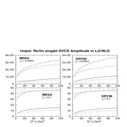
FIG. 1.: The $Q^{2}$-dependence of the real and imaginary parts of the quark singlet DVCS amplitude. The solid (dashed) curve is the real part in LO (NLO) and the dotted (dashed-dotted) curve is the imaginary part in LO (NLO).

The NLO corrections are generally fairly large and tend to decrease the value of the real part and increase the value of the imaginary part of the quark singlet amplitude (bearing in mind that the NLO imaginary amplitude is lower at the input scale, due to the inclusion of the NLO coefficient function). The relative correction, $R$, in moving from LO to NLO (i.e. $R=$ (NLO-LO)/LO)) can be inferred from Fig.(1). $R$ is typically $-20\%$ to $-40\%$ for the real part for both values of $\zeta$. For the imaginary part at $\zeta=0.1$ the corrections are moderate ($|R|<20\%$), whereas at small $\zeta$, $R$ can be as large as $+50\%$ for GRV98 at large $Q^{2}$. The amplitudes drop dramatically in going from small to large $\zeta$ reflecting the strong decrease in the GPDs. They generally increase with increasing $Q^{2}$, albeit moderately, reflecting the expected $\ln(Q^{2})$ behavior. In fact, an approximate scaling is observed at LO and NLO, but only sets in at large $Q^{2}$ for small $\zeta$ in the imaginary part at NLO.

In Fig.(1) and subsequent figures a comparison of the LO and NLO curves at the input scale $Q^{2}=4$ GeV² reveals the effect of including NLO coefficient functions alone. Of course at higher $Q^{2}$ NLO effects are included in both the coefficient functions and in the evolution of the GPDs. For the numerical size of the NLO corrections in the evolution of the GPDs alone see [15].

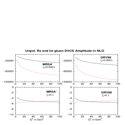
FIG. 2.: The $Q^{2}$-dependence of the real (solid line) and imaginary (dotted line) parts of the unpolarized gluon DVCS amplitude, for two representative values of $\zeta$.

In Fig.(2) we show the real and imaginary parts of the unpolarized gluon amplitude (cf. eq. (40)) which starts at NLO. We note firstly that the gluon contribution is of the same order of magnitude as the quark singlet one, although it is suppressed by $\alpha_{s}/2\pi$ and secondly that both the real and imaginary parts are large and negative. This explains the strong variation of the azimuthal angle asymmetry (AAA), in moving from LO to NLO, observed in [16] (for the case of a dominant Bethe-Heitler contribution) which is directly proportional to the real part of a combination of DVCS amplitudes. Otherwise, the gluon mirrors the NLO quark singlet amplitudes in its behavior in $Q^{2}$ and for large and small $\zeta$.

Of course for the physical amplitude at NLO one must add the quark singlet and gluon contributions together. For the real part at small $\zeta=10^{-4}$ this leads to a relative relative change in moving from LO to NLO of $40\%$ (MRSA’) and $80\%$ (GRV98) at the input scale to $75\%$ (MRSA’) and $80\%$ (GRV98) at $Q^{2}=100$ GeV². For large $\zeta=0.1$ the relative change in the real part at both scales is about $60\%$. For the imaginary part at small $\zeta=10^{-4}$ the relative changes for MRSA’ are $35\%$ (at the input) and $15\%$ (at $Q^{2}=100$ GeV²). For GRV98 one finds $50\%$ (input scale) and $2\%$ (evolved scale) changes. For the imaginary part at large $\zeta=0.1$, for both MRSA’ and GRV98, one finds about $30\%$ (input scale) and $10\%$ (evolved scale) changes. Note that the NLO changes in the physical amplitude decrease as $Q^{2}$ increases in line with the expectation of perturbative QCD that the NLO corrections should die out as $Q^{2}\rightarrow\infty$.

In Fig. (3) we show the ratio of the real to imaginary parts for both the quark singlet and the gluon amplitudes as a function of $Q^{2}$. We note that for small $\zeta$ the ratios can be as large as $45\%$ (a similar value was found for the closely related process of high energy $J/\psi$ photoproduction in [28]). The quark ratios are slightly different for the two inputs. The greatest contrast is seen at small $\zeta$: the NLO case is basically flat in $Q^{2}$ which differs markedly from LO which rises with $Q^{2}$. Both cases are similar at large $\zeta$. The gluon ratio is remarkably similar for the two input sets, at both small and large $\zeta$, for the whole $Q^{2}$ range considered.

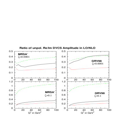
FIG. 3.: The ratio of real to imaginary parts of the unpolarized quark singlet and gluon DVCS amplitudes, as a function of $Q^{2}$. The solid (dotted) curve is for the quark singlet in LO (NLO) and the dashed curve is for the gluon in NLO.

We now turn to the $\zeta$-dependence for fixed $Q^{2}$ which is shown in fig.(4) for the quark singlet and fig.(5) for the gluon. The most striking feature for the quark singlet case is that the amplitudes exhibit an effective power-like behavior in $\zeta$ over basically the whole range ($\zeta\in[0.0001,0.2]$), as illustrated by the straight lines in fig.(4). A simple two parameter fit of the type $a_{0}\zeta^{\lambda_{0}}$ works remarkably well up to about $\zeta=0.1$. The best fit is obtained with a four parameter fit, of the type $c_{1}\zeta^{\lambda_{1}}(1+c_{2}\zeta^{\lambda_{2}})$, which can reproduce most of the curves on the few percent level, with $\lambda_{0}$ and $\lambda_{1}$ within $5\%-20\%$ of each other, and $\lambda_{2}$ small. The simple two parameter fit works best for the imaginary part of the amplitudes where we obtain a value for $\lambda_{0}$ between $-1.1$ and $-1.25$ with a moderate growth in $Q^{2}$ as expected from measurements of the slope of $F_{2}$ and HERA diffractive processes. For the real part of the amplitude the simple fit starts to decrease in quality around $\zeta=0.05$ (depending on the input).

Similar power-like behaviors have been observed in many small-$x$ processes at at HERA, including diffractive DIS in which the $x_{I\!\!P}$-dependence of diffractive structure functions is known to factorize for small $x_{I\!\!P}$. This behavior, known as Regge factorization, is predicted for high energy processes within Regge theory given the postulate of a universally exchanged Regge pole, known as the Pomeron. Since the relationship between the phenomenological Regge Theory and perturbative QCD remains unresolved, we find the observation of this single power in our numerical perturbative QCD calculation remarkable and very interesting.

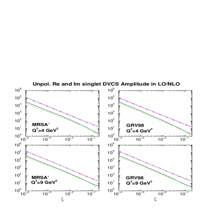
FIG. 4.: The real and imaginary parts of the unpolarized quark singlet DVCS amplitude, as a function of $\zeta$. The solid (dashed) curve is the real part in LO (NLO) and the dotted (dashed-dotted) curve is the imaginary part in LO (NLO). A remarkably simple behaviour is observed in $\zeta$ which is close to a single power over a wide range. Because $Q^{2}$ is fixed, this behaviour in $\zeta$ translates directly into a single power in energy.

Note that we do not claim to have derived this powerlike behaviour from first principles. The analytic forms for the coefficients functions (see appendix VI A) would seem to favor a more complicated sum of logs in $\zeta$, particularly when the interplay with the effective behaviour in $\zeta$ of the GPDs, at a given $Q^{2}$, is taken into account. Hence, the fact that a single power apparently works for such a large range in $\zeta$ for DVCS is somewhat surprising. Naively one may expect that a sum of two or more powers would be required to give a reasonable fit. Perhaps this indicates that DVCS always proceeds through partonic configurations which lie in the same universality class, i.e. are self-similar. The reason why these self-similar configuration seem to be of importance beyond the “diffractive region” can be understood if one examines the behavior of the integrand in the convolution integrals in eqs. (32, 40). One observes that a large contribution to the integral and ultimately to the imaginary part of the amplitude itself stems from the region in $X$ very close to $\zeta$, even for larger values of $\zeta$, leading to the self-similar behavior. This is not too surprising given the steep rise of the GPD in the DGLAP region towards $\zeta$ and that the coefficient functions are singular at $\zeta$, where even the implementation of the principal value in Sec. (II) leaves an integrable singularity.

This situation is somewhat altered for the real part of the amplitude where the ERBL region plays a very important part, as we will see. There, although the coefficient function is singular, the symmetry of the GPD in the ERBL region makes the value of the integral somewhat less dependent on the region near $\zeta$, i.e. less singular, especially for large $\zeta$. Although the value of the real part also depends on an integral over the DGLAP region which contributes more to the power like behavior, this dependence progressively decreases as $\zeta$ grows.

The physical picture which is emerging is the following: the region near $\zeta$ corresponds to large light-cone distances for the operators which translates into two parton configurations, either a $q\bar{q}$ pair in the ERBL region or a quark leaving and then returning to the proton in the DGLAP region, where one of the partons, either the $\bar{q}$ or the returning $q$, carries virtually zero momentum fraction, $X-\zeta$, in either the $+$ or $-$ direction on the light cone and the other carries approximately $\zeta$, i.e. very asymmetric configurations seem to have a disproportionate weighting in the amplitude. The coefficient functions, with their singularity structure at $\zeta$, weight these configurations much more heavily in the amplitude than other, more symmetric, configurations.

Although asymmetric configurations become rare as one approaches the valence region of large $\zeta$, because they should be mainly found in the sea, they are still enhanced by the singularity structure of the coefficient functions. This then leads us to the conclusion that, although the sea is small at large $\zeta$, DVCS still proceeds largely through sea configurations in the valence region, thus its relative scarcity compared to DIS in the valence region. Physically, at large $X\approx\zeta$, one has to strike an unusual fluctuation in the proton to emit a real photon, while still leaving the proton intact.

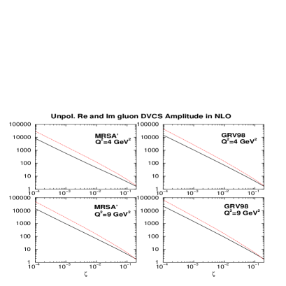
FIG. 5.: The modulus of the real and imaginary parts of the unpolarized gluon DVCS amplitude as functions of $\zeta$, for fixed $Q^{2}$. The solid curve is the modulus of the real part and the dotted curve is the modulus of the imaginary part of the gluon amplitude.

For the gluon contribution, shown in Fig.(5), we find the same behavior as in the case of the quark singlet. Note that we took the modulus of both the real and imaginary parts, since they are actually negative, in order to produce a log-log plot. Performing the same type of fits as in the quark case, one obtains similar numbers for $\lambda_{0}$ between $-1.14$ and $-1.28$ in the two parameter fit and again very similar ones in the four parameter fit ($5\%-25\%$ variation in the powers). The quality of the two parameter fit starts to decrease rapidly for a $\zeta\sim 0.05$. Nevertheless, the explanation given in the quark singlet case is still applicable in the case of the gluon.

In Fig. (6) we show the ratio of real to imaginary parts in $\zeta$ for fixed $Q^{2}$. Again we note the remarkable similarity between the gluon curves for both inputs, both in shape as well as absolute values. A very mild growth is seen for the quark singlet ratio in $\zeta$, whereas the gluon varies quite strongly in $\zeta$.

Using Fig. (6) we can make a simple test to check whether we have computed the real part of the amplitude at small $\zeta$ properly by employing a dispersion relation for the unpolarized amplitudes at small $\zeta$ (for more details see [28]):

$$\frac{\mbox{Re}~{}T_{DVCS}}{\mbox{Im}~{}T_{DVCS}}=\tan\left(\frac{\pi}{2}(|\lambda|-1)\right)\,.$$ (41)

For the fitted values of $\lambda$ we obtain a ratio which is in very good agreement with the values in Fig. (6) up to about $\zeta=5\times 10^{-3}$ for both the quark singlet and the gluon. This confirms the self-consistency of our calculation.

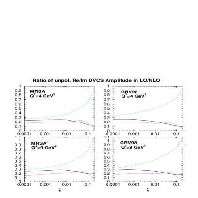
FIG. 6.: The ratio of real to imaginary parts of the unpolarized quark singlet and gluon DVCS amplitude, as a function of $\zeta$, at fixed $Q^{2}$. The solid (dotted) curve is the ratio in LO (NLO) and the dashed curve is the ratio for the gluon in NLO.

Next we discuss the relative importance of the ERBL region to the value of the real part of the DVCS amplitude, starting with the quark singlet. On inspection of the relative contribution of the ERBL integrals ($X\in[0,\zeta]$) in eqs. (32, 40) we find that at small $\zeta$ the ERBL region integral has a relative contribution between $90\%$ at the input scale and $140\%$ at $Q^{2}=100~{}\mbox{GeV}^{2}$ ($100\%$ and $50\%$ respectively in LO) of the value of the amplitude, i.e. there is a large cancellation between the subtraction term and the $X\in[\zeta,1]$ integral with both of them being substantially larger, individually than the $[0,\zeta]$ integral. As one increases $\zeta$ the relative importance of the ERBL region drops to $50\%$ at the input scale and $130\%$ at $Q^{2}=100~{}\mbox{GeV}^{2}$ ($80\%$ and $30\%$ respectively in LO), however, the subtraction term now starts to dominate the value of the amplitude. This observation is in line with our previous argument of the importance of very asymmetric parton configurations. Remember, that the subtraction term is directly proportional to the GPD at $\zeta$. Also note that going from LO to NLO seems to change the relative importance of the ERBL region, especially its $Q^{2}$ behavior.

Turning now to the gluon we make a slightly different observation. Firstly, at small $\zeta$ the relative contribution varies from $40\%-60\%$ in going from the input scale to $Q^{2}=100~{}\mbox{GeV}^{2}$ again there is a large cancellation between the previously mentioned terms, but the change in $Q^{2}$ is not very dramatic. Increasing $\zeta$ one finds an increase of the relative importance to $60\%-80\%$ in going from the input scale to our large $Q^{2}$ value. Again the subtraction term becomes more and more dominant, relatively speaking, and thus our interpretation from the quark case carries over to the gluon case.

To close our analysis of the unpolarized case, we discuss the scale dependence of the DVCS amplitudes. We varied the factorization scale, $\mu^{2}$, from $Q^{2}$, used above, to $Q^{2}/2$ and $2Q^{2}$ for both sets and found the following variations, where the two sets agree fairly well with one another. At small $\zeta$, we found a small variation at the input scale of $3-5\%$ which increases to about $15\%-30\%$ at large $Q^{2}$ (we used $Q^{2}=100~{}\mbox{GeV}^{2}$, for the large scale, throughout) for both real and imaginary part of the quark singlet. For the gluon we find a variation of about $15\%$ for the real and imaginary part at the input scale which reduces to about $10\%$ for the real part and to about $2\%$ for the imaginary part. At large $\zeta$, we find similar variations as the authors of [19], i.e. around $5\%$ for both the real and imaginary parts of the quark singlet and around $10\%$ for the gluon, for both the input scale and at large $Q^{2}$. In summary one can say that the scale dependence is not troublesome and that the uncertainties due to the chosen GPD are still much larger than those due to the factorization scale.

B The polarized case

For the polarized case we proceed exactly as we did for the unpolarized case starting in Fig. (7) with the absolute values of the real and imaginary parts of the polarized quark singlet amplitudes as functions of $Q^{2}$. Again the relative impact of the NLO corrections to the quark singlet can be inferred from this figure. One immediately notices for small $\zeta$ the very large NLO corrections for the GS(A) input ($|R|$ can be as large as $70\%$), whereas for the GRSV00 input (‘standard scenario’, i.e. unbroken sea) the corrections are more moderate ($|R|<20\%$). The very large corrections can be easily explained since in [15] it was shown that the GPD evolution drastically alters the shape of the GS(A) distribution in fact inverting its shape, whereas the shape of GRSV00 was almost unchanged and the absolute value changed only moderately. The difference in shape at small $\zeta$ was due to radically different assumptions about the polarized sea distribution. At large $\zeta$, where the shape of the two input sets is similar we find that the shape of the amplitudes in $Q^{2}$ is also very similar, whereas their absolute values differ.

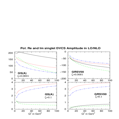
FIG. 7.: Real and imaginary parts of the polarized quark singlet DVCS amplitude, as a function of $Q^{2}$, for fixed $\zeta$. The solid (dashed) curve is the real part in LO (NLO) and the dotted (dashed-dotted) curve is the imaginary part in LO (NLO).

The real and imaginary parts of the polarised gluon amplitude are plotted in Fig. (8). Note that the real and imaginary parts of the amplitude are positive for small $\zeta$, exactly the opposite to the unpolarized case. For large $\zeta$, the real parts are positive, again in contrast to the unpolarised case. The imaginary part at large $\zeta$ starts positive but becomes negative under evolution. This behavior is due to the particular shape of the polarized gluon GPD at small and large $\zeta$ (see [15]).

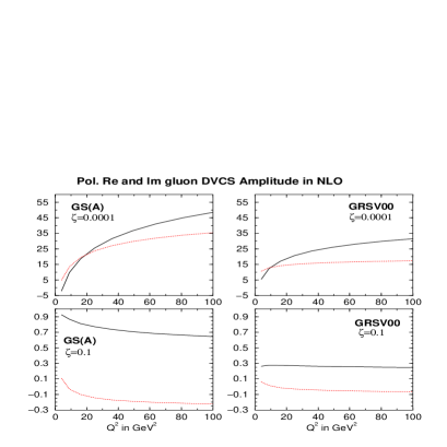
FIG. 8.: The real and imaginary parts of the polarized gluon DVCS amplitude, as a function of $Q^{2}$, for fixed $\zeta$. The solid curves show the real part and the dotted curves show the imaginary part of the gluon amplitude.

In Fig.(9) we show the ratio of real to imaginary parts as a function of $Q^{2}$, for fixed $\zeta$. At large $\zeta$, we again observe flattening at large $Q^{2}$: the GRSV00 result is flatter than the GS(A) case, especially at NLO, where we still observe strong variations in $Q^{2}$. For large $Q^{2}$, the gluon ratio is very similar for both sets and fairly flat in $Q^{2}$. We did not plot the gluon ratio at large $\zeta$ since it has a very large value near the point where the imaginary part changes sign and thus would have completely swamped the quark result which we find more interesting here. Note that our LO ratio for the GS(A) model is in agreement with the values obtained in [18].

In Fig. (10) we plot the $\zeta$-behaviour at fixed $Q^{2}$ and find a single power-like behaviour only for very small $\zeta$ (up to about $3\times 10^{-3}$), seen explicitly on the log-log plot for GS(A). Performing the same type of fits as in the unpolarized case, i.e. a simple two and four parameter fits, reveals a $\lambda_{0}$ between $-0.4$ to $-0.55$, and a similar story for the four parameter fits. However, the second power, $a_{2}$, is now substantially larger than in the unpolarized case, in order to be able to describe the large $\zeta$ behavior. The four parameter fit is able to describe the behavior of the amplitudes on the few percent level. Thus the simple single-power Regge-type effective behavior observed in the unpolarized case is only valid at small $\zeta$ in the polarized case. This is because the polarized sea dies out even more quickly with increasing $\zeta$, than the unpolarized one: therefore the highly asymmetric configurations necessary to produce a universal behavior in $\zeta$ become very rare. At large $\zeta$ they are almost completely gone.

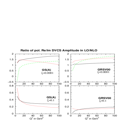
FIG. 9.: The ratio of real to imaginary parts of the polarized quark singlet and gluon DVCS amplitudes, as a function of $Q^{2}$, at fixed $\zeta$. The solid (dotted) curves show the ratio for the quark singlet in LO (NLO) and the dashed curves show the ratio for the gluon in NLO.

FIG. 10.: Polarized real and imaginary parts of the quark singlet DVCS amplitude, as a function of $\zeta$, for fixed $Q^{2}$. The solid (dashed) curve is the real part in LO (NLO) and the dotted (dashed-dotted) curve is the imaginary part in LO (NLO).

Turning to the gluon in Fig. (11) we illustrate that the behavior in $\zeta$ at an evolved scale, $Q^{2}=9$ GeV², is very similar in shape and size for the two input sets, despite the fact that they start off very different at the input scale, $Q^{2}=4$ GeV². The evolution forces the distributions to be quite similar very quickly.

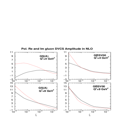
FIG. 11.: Real and imaginary parts of the polarized gluon DVCS amplitude, as a function of $\zeta$, at fixed $Q^{2}$. The solid curve is the real part in NLO and the dotted curve is the imaginary part.

For the GS(A) input, at small $\zeta$, the relative changes in going from LO to NLO in the physical polarized amplitude, i.e. the sum of polarized quark singlet and polarized gluon, are found to be about $15\%$ for both the real and imaginary parts at the input scale and about $8\%$ for the imaginary part and $40\%$ for the real part at $Q^{2}=100$ GeV². At large $\zeta=0.1$, the changes in the real part vary from about $90\%$ at the input scale to $25\%$ at $Q^{2}=100$ GeV² and those in the imaginary part vary from about $25\%$ (at the input scale) to $15\%$ at the evolved scale. For GRSV00 we also find a decrease in the variation which at small $\zeta$ drops from $60\%$ at the input scale to $25\%$ at $Q^{2}=100$ GeV² for the imaginary part, and from $35\%$ to $5\%$ for the real part. At large $\zeta$ there is a decrease from about $25\%$, at the input for both real and imaginary parts, to about $2\%$ and $15\%$ for the real and imaginary parts, respectively, at the evolved scale. As in the unpolarized case the NLO corrections to the physical amplitude decrease as $Q^{2}$ increases except in the case of the real part at small $\zeta$ for GS(A) which is in line with the dramatic NLO evolution effects in the ERBL region.

The relative change induced by NLO corrections of the quark singlet can be inferred directly from Fig. 10.

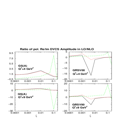
FIG. 12.: The ratio of real to imaginary parts of the polarized quark singlet and gluon DVCS amplitudes, as a function of $\zeta$ at fixed $Q^{2}$. The solid (dotted) curve is the ratio in LO (NLO) and the dashed curve is the ratio for the gluon, which starts at NLO.

The $\zeta$-dependence of the ratio of real to imaginary parts, plotted in Fig. (12), is rather different to the unpolarized case, with a strong fluctuation in the gluon due to a sign change of one of the amplitudes around the spike (we sample at a finite number of points in $\zeta$). The real part is typically much larger then the imaginary part, in contrast to the unpolarized case.

Concerning the issue of the importance of the ERBL region, we find a similar picture to the unpolarized case, although the relative percentage contribution is smaller by about a factor of two, for both quarks and gluons. The influence of the subtraction term on the value of the real part of the amplitude is considerably less than in the unpolarized case, thus the ERBL region is weighted more heavily in the final value of the amplitude. This is in line with our observation of the deviations of the amplitudes from a single power in $\zeta$, for relatively small values of $\zeta$, compared to the unpolarized case (for which the ERBL region was of less importance as compared to the subtraction term).

Finally, we comment briefly on the factorization scale dependence of the polarized amplitudes. We proceed in an identical manner to the unpolarized case in varying $\mu^{2}$. For small $\zeta$, we find a similar variation as in the unpolarized case for the quark singlet and larger variations of $35-40\%$ at the input scale and $1-30\%$ at large $Q^{2}=100$ GeV², respectively, for the gluon. At large $\zeta$, we find variations in the real part of the quark singlet around $100\%$ at the input and at large $Q^{2}$. The imaginary part only varies between $5\%$ at the input scale to $20\%$ at the evolved scale. Both real and imaginary parts of the gluon amplitude at large $\zeta$ are very well behaved and vary only between $5-20\%$ at both the input scale and at large $Q^{2}$. It is encouraging that the variations due to factorization scale changes can be safely neglected since the polarized distributions are even less well known than the unpolarized ones.

IV General comments on NLO and NNLO corrections

In this section we make some general comments about the structure of NLO corrections and expected NNLO corrections.

In [15] we pointed out that the relative shape change in the NLO evolution of GPDs, compared with LO, is due to a new class of integrable divergences, $\ln\left(1-X/\zeta\right)^{n}/(1-X/\zeta)^{i},~{}\mbox{n,i}=0,1,2$, appearing in the region around $\zeta$. The same type of integrable divergence also appears in the NLO coefficient functions, but is absent at LO, although one has an integrable singularity of the $1/(1-X/\zeta)$ type. This fact alone helps to explain why one finds, in certain regions, large changes in going from LO to NLO in the amplitudes.

For DVCS observables the appearance of the gluon at NLO also changes things dramatically since the gluon contribution turns out to be of the same order as the quarks, at least at small $\zeta$ due to an extra factor of $1/\zeta$ in eq. (20). So, not only is a new quantity introduced, but one of the same order of magnitude as our LO quantities. Furthermore, with the unpolarized real part of the gluon amplitude being negative and of comparable size at small $\zeta$ as the NLO correction to the real part of the quark amplitudes (which is also negative), observables sensitive to the real part, such as the azimuthal angle asymmetry are expected to change dramatically in NLO (see [16]). Conversely, the effect should not be as dramatic for observables sensitive to the imaginary part, despite the fact that the NLO gluon correction is big and negative, since the correction to the quark singlet at NLO is big and positive so the corrections will cancel to a certain extent (see [16]).

What would one expect in NNLO ? From experience obtained in calculating forward coefficient functions, and some evolution kernels at ${\cal O}(\alpha^{2}_{s})$, one would expect to see only the same type of integrable divergences reappearing, maybe with different powers in logs and rational functions, but not a new class of divergences which could radically alter the behavior of the amplitudes. Also, in contrast to moving from LO to NLO which gives the first gluon contributions, no new parton species appears at NNLO. This leads us to speculate that the NNLO order corrections should be mild.

V Conclusions

We have presented a detailed analysis of the quark singlet and gluon contributions to the polarized and unpolarized DVCS amplitudes at NLO, using NLO-evolved generalised partons distributions (GPDs) built from sensible input models. We have compared throughout with the LO results using the same input GPDs, and have therefore quantized the effect of the NLO corrections.

These results are directly relevant to measurable quantities in $ep\rightarrow ep\gamma$ processes at the HERA and HERMES experiments, and hence may be used to constrain the GPDs at NLO.

The most striking feature of our results is that for a given $Q^{2}$ the unpolarized amplitudes exhibit an effective single-power behaviour in the skewedness parameter, $\zeta$, over a very large range, apparently indicating a universal behaviour.

VI Appendix

A LO and NLO coefficient functions

The coefficient functions in eq. (20) are expanded in powers of $\alpha_{s}$. Up to terms of ${\cal O}(\alpha^{2}_{s})$, they read

$$T^{q,V/A}(z)= T^{q,LO}(z)+\frac{\alpha_{s}(\mu^{2})}{2\pi}T^{q,NLO,V/A}(z,Q^{2}/\mu^{2})\,,$$ (42)

$$T^{g,V/A}(z)= T^{g,LO}(z)+\frac{\alpha_{s}(\mu^{2})}{2\pi}T^{g,NLO,V/A}(z,Q^{2}/\mu^{2})\,,$$ (43)

with $z=2X/\zeta-1$.

The LO and NLO coefficient functions were taken from [19] and are given by:

$$T^{q,LO}(z)=\frac{1}{1-z},$$ (44)

$$T^{g,LO}(z)=0,$$ (45)

$$T^{q,NLO,V}(z)=T^{q,NLO,A}(z)-\frac{C_{F}}{1+z}\ln\frac{1-z}{2},$$ (46)

$$T^{q,NLO,A}(z)=\frac{C_{F}}{2(1-z)}\Big{[}\left(2\ln\frac{1-z}{2}+3\right)\times$$ (47)

$$\left(\ln\frac{Q^{2}}{\mu^{2}}+\frac{1}{2}\ln\frac{1-z}{2}-\frac{3}{4}\right)-\frac{27}{4}-\frac{1-z}{1+z}\ln\frac{1-z}{2}\Big{]}\,,$$ (48)

$$T^{g,NLO,V}(z)=-T^{g,NLO,A}(z)+$$ (49)

$$\frac{N_{F}}{2}\Big{[}\frac{1}{1-z}\left(\ln\frac{Q^{2}}{\mu^{2}}+\ln\frac{1-z}{2}-2\right)+\frac{\ln\frac{1-z}{2}}{1+z}\Big{]}\,,$$ (50)

$$T^{g,NLO,A}(z)=\frac{N_{F}}{2}\Big{[}\left(\frac{1}{1-z^{2}}+\frac{\ln\frac{1-z}{2}}{(1+z)^{2}}\right)\times$$ (51)

$$\left(\ln\frac{Q^{2}}{\mu^{2}}+\ln\frac{1-z}{2}-2\right)-\frac{\ln^{2}\frac{1-z}{2}}{2(1+z)^{2}}\Big{]},$$ (52)

where the LO quark coefficient is normalized in such a way that, in the forward limit, after properly restoring the dependence on both skewedness parameters, one recovers the LO DIS coefficient $\delta(1-x)$ and the NLO gluon coefficient is normalized such that one recovers $\frac{1}{2}C^{DIS}_{g}$.

In the interval $[0,\zeta]$, the above coefficients are strictly real. However, in the interval $[\zeta,1]$, they split into a real and imaginary parts, which can be easily deduced from eq. (52).

B LO and NLO subtraction functions

In this section, we present the subtraction functions needed in our implementation of the Cauchy principal value prescription of eq.(24), i.e. the integrals

$$I^{q,V/A}(\zeta)=\int^{1}_{0}dX~{}T^{q,V/A}\left(\frac{2X}{\zeta}-1\right)\,,$$ (53)

$$I^{g,V/A}(\zeta)=\int^{1}_{0}dX~{}T^{g,V/A}\left(\frac{2X}{\zeta}-1\right)\,.$$ (54)

There are four different integrals to be done, which are regulated by adding $+i\epsilon$ to $X$ (this implies analytically continuing the log terms in the lower half plane to pick up $-i\pi$). This generates real and imaginary parts for the subtraction functions, $I^{q,g}$, given below, for the unpolarised (V) and polarised (A) cases. One has to be careful to take the appropriate sheet of the Riemann surface for the logarithms in order to obtain the correct imaginary parts, i.e. to use the $+i\epsilon$ prescription consistently. In order to ensure the correctness of the results below, we cross checked them both with MATHEMATICA and MAPLE.

$$I^{q,LO}(\zeta)=-\frac{\zeta}{2}\Big{[}\ln\left(\frac{1-\zeta}{\zeta}\right)-i\pi\Big{]}\,,$$ (55)

$$I^{q,NLO,A}(\zeta,Q^{2},\mu^{2})=\frac{C_{F}\zeta}{4}\Bigg{[}\frac{\pi^{2}}{6}-\mbox{Li}_{2}\left(1-\frac{1}{\zeta}\right)+$$ (56)

$$\ln\left(\frac{1-\zeta}{\zeta}\right)(\pi^{2}+9+\ln\zeta-\frac{1}{3}\ln^{2}\left(\frac{1-\zeta}{\zeta}\right))+$$ (57)

$$\ln\frac{Q^{2}}{\mu^{2}}\left(\pi^{2}-3\ln\left(\frac{1-\zeta}{\zeta}\right)-\ln^{2}\left(\frac{1-\zeta}{\zeta}\right)\right)-$$ (58)

$$i\pi\Big{[}\frac{\pi^{2}}{3}+9+\ln\zeta-\ln^{2}\left(\frac{1-\zeta}{\zeta}\right)-$$ (59)

$$\quad\ln\frac{Q^{2}}{\mu^{2}}\left(2\ln\left(\frac{1-\zeta}{\zeta}\right)+3\right)\Big{]}\,\Bigg{]},$$ (60)

$$I^{q,NLO,V}(\zeta,Q^{2},\mu^{2})=\frac{C_{F}\zeta}{4}\Bigg{[}\frac{\pi^{2}}{2}-3\mbox{Li}_{2}\left(1-\frac{1}{\zeta}\right)+$$ (61)

$$\ln\left(\frac{1-\zeta}{\zeta}\right)(\pi^{2}+9+3\ln\zeta-\frac{1}{3}\ln^{2}\left(\frac{1-\zeta}{\zeta}\right))+$$ (62)

$$\ln\frac{Q^{2}}{\mu^{2}}\left(\pi^{2}-3\ln\left(\frac{1-\zeta}{\zeta}\right)-\ln^{2}\left(\frac{1-\zeta}{\zeta}\right)\right)-$$ (63)

$$i\pi\Big{[}\frac{\pi^{2}}{3}+9+3\ln\zeta-\ln^{2}\left(\frac{1-\zeta}{\zeta}\right)-$$ (64)

$$\quad\ln\frac{Q^{2}}{\mu^{2}}\left(2\ln\left(\frac{1-\zeta}{\zeta}\right)+3\right)\Big{]}\,\Bigg{]}\,,$$ (65)

$$I^{g,NLO,A}(\zeta,Q^{2},\mu^{2})=\frac{N_{F}\zeta}{4}\Bigg{[}1+\frac{\pi^{2}\zeta}{4}+$$ (66)

$$\zeta\ln\left(\frac{1-\zeta}{\zeta}\right)(1-\frac{1}{4}\ln\left(\frac{1-\zeta}{\zeta}\right))-$$ (67)

$$\frac{1}{2}\ln\frac{Q^{2}}{\mu^{2}}\left(1+\zeta\ln\left(\frac{1-\zeta}{\zeta}\right)\right)-$$ (68)

$$\frac{i\pi\zeta}{2}\Big{[}2-\ln\left(\frac{1-\zeta}{\zeta}\right)-\ln\frac{Q^{2}}{\mu^{2}}\Big{]}\,\Bigg{]},$$ (69)

$$I^{g,NLO,V}(\zeta,Q^{2},\mu^{2})=\frac{N_{F}\zeta}{4}\Bigg{[}-1+\frac{\pi^{2}}{3}\left(1-\frac{3\zeta}{4}\right)+$$ (70)

$$\mbox{Li}_{2}\left(1-\frac{1}{\zeta}\right)-\ln\zeta\ln\left(\frac{1-\zeta}{\zeta}\right)+$$ (71)

$$(2-\zeta)\ln\left(\frac{1-\zeta}{\zeta}\right)(1-\frac{1}{4}\ln\left(\frac{1-\zeta}{\zeta}\right))+$$ (72)

$$\frac{1}{2}\ln\frac{Q^{2}}{\mu^{2}}\left(1-(2-\zeta)\ln\left(\frac{1-\zeta}{\zeta}\right)\right)-$$ (73)

$$\frac{i\pi}{2}\Big{[}(2-\zeta)\left(2-\ln\frac{Q^{2}}{\mu^{2}}-\ln\left(\frac{1-\zeta}{\zeta}\right)\right)-2\ln\zeta\Big{]}\Bigg{]}.$$ (74)

REFERENCES

- [1] D. Müller et al., Fortsch. Phys. 42 (1994) 101.
- [2] A. V. Radyushkin, Phys. Rev. D 56 (1997) 5524.
- [3] X. Ji, Phys. Rev. D55 (1997) 7114; J. Phys. G 24 (1998) 1181.
- [4] M. Diehl et al., Phys. Lett. B 411 (1997) 193.
- [5] M. Vanderhaeghen, P. A. M. Guichon and M. Guidal, Phys. Rev. D 60 (1999) 094017.
- [6] J. C. Collins and A. Freund, Phys. Rev. D 59 (1999) 074009.
- [7] X. Ji. and J. Osborne, Phys. Rev. D 58 (1998) 094018.
- [8] L. Frankfurt, A. Freund and M. Strikman, Phys. Rev. D 58 (1998) 114001; Erratum-ibid. D59 (1999) 119901 and Phys. Lett. B 460 (1999) 417, A. Freund and M. Strikman, Phys. Rev. D 60 (1999) 071501.
- [9] A. Airapetian et al., HERMES Collab., hep-ex/0106068; P.R. Saull, for ZEUS Collab., hep-ex/0003030; L. Favart, for H1 and ZEUS Collabs., hep-ex/0106067; J. P. Chen, for Jefferson Lab, http://www.jlab.org/sabatie/dvcs/index.html.
- [10] A. V. Belitsky et al., Phys. Lett. B 437 (1998) 160; A. V. Belitsky, A. Freund and D. Müller, Nucl. Phys. B574 (2000) 347.
- [11] V. Yu. Petrov et al., Phys. Rev. D 57 (1998) 4325.
- [12] L. Frankfurt et al., Phys. Lett. B 418 (1998) 345, Erratum-ibid. B429 (1998) 414; A. Freund and V. Guzey, Phys. Lett. B 462 (1999) 178.
- [13] V. N. Gribov and L. N. Lipatov, Sov. J. Phys 15 (1972) 438, 675; Yu. L. Dokshitzer, Sov. Phys. JETP 46 (1977) 641; G. Altarelli. and G. Parisi, Nucl Phys B126 (1977) 298.
- [14] A. V. Efremov and A. V. Radyushkin, Theor. math. Phys. 42 (1980) 97, Phys Lett. B94 (1980) 245; S. J. Brodsky and G. P. Lepage, Phys Lett. B87 (1979) 359; Phys. Rev. D22 (1980) 2157.
- [15] A. Freund and M. McDermott, hep-ph/0106115.
- [16] A. Freund and M. McDermott, hep-ph/0106124.
- [17] A. V. Belitsky et al., Phys. Lett. B 510 (2001) 117.
- [18] A. V. Belitsky et al., Nucl. Phys. B 593 (2001) 289.
- [19] A. V. Belitsky et al., Phys. Lett. B 474 (2000) 163.
- [20] K. Golec-Biernat and A. D. Martin, Phys. Rev. D 59 (1999) 014029.
- [21] A. V. Radyushkin, Phys. Rev. D59 (1999) 014030.
- [22] N. Kivel, M. V. Polyakov and M. Vanderhaeghen, Phys. Rev. D 63 (2001) 114014.
- [23] M. V. Polyakov and C. Weiss, Phys. Rev. D 60 (1999) 114017.
- [24] M. Glück, E. Reya and A. Vogt, Eur. Phys. J. C 5 (1998) 461; M. Glück et al., Phys.Rev. D63 (2001) 094005; We evolve from the low input scales up to GeV, using conventional (forward) DGLAP evolution.
- [25] A. D. Martin, R. G. Roberts and W. J. Stirling, Phys. Lett. B 354 (1995) 155; T. Gehrmann, W. J. Stirling, Phys. Rev. D 53 (1996) 6100.
- [26] J. Blumlein, B. Geyer and D. Robaschik, Phys. Lett. B406 (1997) 161; I. I. Balitsky and A. V. Radyushkin, Phys. Lett. B413 (1997) 114; L. Mankiewicz et al., Phys. Lett. B 425 (1998) 186; A. V. Belitsky and D. Mueller, Phys. Lett. B 417 (1998) 129, Nucl. Phys. B 537 (1999) 397.
- [27] A. Freund and M. McDermott, “A detailed next-to-leading order QCD analysis of deeply virtual Compton scattering observables”, hep-ph/0111472.
- [28] L. Frankfurt, M. McDermott and M. Strikman, JHEP 0103 (2001) 045.