NEW MODEL FOR THE QCD
ANALYTIC RUNNING COUPLING

As an elaboration of the analytic approach to Quantum Chromodynamics (QCD), a new model for the QCD analytic running coupling is proposed. A self-evident advantage of the new analytic running coupling (NARC) is that it incorporates the infrared enhancement and the ultraviolet asymptotic freedom in a single expression. It is essential that additional parameters are not introduced in the theory. The absence of unphysical singularities in the physical region $q^{2}>0$ and a fairly well loop and scheme stability are the remarkable features of the NARC. By making use of practically the same values of $\Lambda_{\mbox{\tiny QCD}}$ in the approach developed, one succeeded in description of various physical phenomena, from quark confinement to the $\tau$ lepton decay. This undoubtedly implies that the new analytic running coupling substantially involves both the nonperturbative and the perturbative behavior of Quantum Chromodynamics.

1 Introduction

The discovering of the asymptotic freedom phenomenon in Quantum Chromodynamics (QCD) led to the wide using of the perturbation theory. The latter gives good results in the ultraviolet (UV) region, but the perturbation theory is absolutely unapplicable in the infrared (IR) region. So, for the description of a number of physical phenomena one needs to use the nonperturbative methods. The current consideration relies on the analytic approach to QCD.

The analytic approach to Quantum Field Theory (QFT) is a nonperturbative method which is based solely on the first principles of the local QFT. First it was formulated on the example of Quantum Electrodynamics in the late 1950’s in the papers.$\!{}^{{\bf?},{\bf?}}$ The basic idea of this approach is the explicit imposition of the causality condition, which implies the requirement of the analyticity in the $q^{2}$ variable for the relevant physical quantities. This approach has recently been extended to QCD $\!{}^{{\bf?}}$ and applied to the “analytization” of the perturbative series for the QCD observables.$\!{}^{{\bf?}}$ The term “analytization” means the recovering of the proper analytic properties in the $q^{2}$ variable by making use of the Källén–Lehmann spectral representation

$$\Bigl{\{}\mbox{\sf A}(q^{2})\Bigr{\}}_{\mbox{$\!${\small an}}}\equiv\int_{0}^{\infty}\!\frac{\varrho(\sigma)}{\sigma+q^{2}}\,d\sigma,$$ (1)

where the spectral density is determined by the initial (perturbative) expression for some quantity A$(q^{2})$:

$$\varrho(\sigma)\equiv\frac{1}{2\pi i}\lim_{\varepsilon\to 0_{+}}\Bigl{[}\mbox{\sf A}(-\sigma-i\varepsilon)-\mbox{\sf A}(-\sigma+i\varepsilon)\Bigr{]},\quad\sigma\geq 0.$$ (2)

2 New Analytic Running Coupling

First of all, let us consider the renormalization group (RG) equation for the invariant charge $g(\mu)$

$$\frac{d\,\ln\bigl{[}g^{2}(\mu)\bigr{]}}{d\,\ln\mu^{2}}=\beta\Bigl{(}g(\mu)\Bigr{)}.$$ (3)

In accordance with the perturbative approach one expands the $\beta$ function on the right hand side of Eq. (3) as a power series

$$\beta\Bigl{(}g(\mu)\Bigr{)}=-\left\{\beta_{0}\left[\frac{g^{2}(\mu)}{16\pi^{2}}\right]+\beta_{1}\left[\frac{g^{2}(\mu)}{16\pi^{2}}\right]^{2}+\ldots\right\},$$ (4)

where $\beta_{0}=11-2\,n_{\mbox{\scriptsize f}}\,/\,3,\,\beta_{1}=102-38\,n_{\mbox{\scriptsize f}}\,/\,3$, and $n_{\mbox{\scriptsize f}}$ is the number of active quarks. Introducing the standard notations ${\alpha}_{\mbox{\scriptsize s}}(\mu^{2})=g^{2}(\mu)/(4\pi)$ and $\widetilde{\alpha}(\mu^{2})=\alpha(\mu^{2})\,\beta_{0}/(4\pi)$, one can reduce the RG equation at the $\ell$-loop level to the form

$$\frac{d\,\ln\bigl{[}\widetilde{\alpha}^{(\ell)}_{\mbox{\scriptsize s}}(\mu^{2})\bigr{]}}{d\,\ln\mu^{2}}=-\sum_{j=0}^{\ell-1}\beta_{j}\left[\frac{\widetilde{\alpha}^{(\ell)}_{\mbox{\scriptsize s}}(\mu^{2})}{\beta_{0}}\right]^{j+1}.$$ (5)

It is well-known that the solution to this equation has unphysical singularities at any loop level. So, there is the ghost pole at the one-loop level, and the account of the higher loop corrections just introduces the additional singularities of the cut type into the expression for the running coupling. But we know from the first principles that the QCD running coupling must have the correct analytic properties in the $q^{2}$ variable, namely, there should be the only left cut-off along the negative semiaxis of $q^{2}$.

So, what is missing in the $\beta$ function perturbative expansion? How one could try to improve the situation? This objective can be achieved by involving into consideration the analytic properties in the $q^{2}$ variable of the RG equation. The perturbative expansion of the $\beta$ function as a power series (4) leads to the violation of the correct analytic properties of the RG equation (3). Thus, one can improve the $\beta$ function perturbative expansion by applying the analytization procedure to it.$\!{}^{{\bf?}}$ This results in the equation

$$\frac{d\,\ln\bigl{[}{{}^{\mbox{\tiny N}}}\!\widetilde{\alpha}^{(\ell)}_{\mbox{\scriptsize an}}(\mu^{2})\bigr{]}}{d\,\ln\mu^{2}}=-\left\{\sum_{j=0}^{\ell-1}\frac{\beta_{j}}{\beta_{0}^{j+1}}\Bigl{[}\widetilde{\alpha}^{(\ell)}_{\mbox{\scriptsize s}}(\mu^{2})\Bigr{]}^{j+1}\right\}_{\mbox{$\!\!$\small an}},$$ (6)

which solution is by definition $\!{}^{{\bf?},{\bf?}}$ the $\ell$-loop new analytic running coupling, ${{}^{\mbox{\tiny N}}}\!\alpha^{(\ell)}_{\mbox{\scriptsize an}}(q^{2})$. In fact, the solution to Eq. (6) is determined up to a constant factor, but this ambiguity can easily be avoided by imposing the physical condition of the asymptotic freedom ${{}^{\mbox{\tiny N}}}\!\alpha^{(\ell)}_{\mbox{\scriptsize an}}(q^{2})\to\alpha^{(\ell)}_{\mbox{\scriptsize s}}(q^{2})$, when $q^{2}\to\infty$. At the one-loop level Eq. (6) can be integrated explicitly with the result

$${{}^{\mbox{\tiny N}}}\!\alpha^{\mbox{\scriptsize(1)}}_{\mbox{\scriptsize an}}(q^{2})=\frac{4\pi}{\beta_{0}}\,\frac{z-1}{z\,\ln z},\qquad z=\frac{q^{2}}{\Lambda^{2}}.$$ (7)

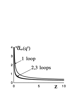
Figure 1: The new analytic running coupling at different loop levels, $z=q^{2}/\Lambda^{2}$.

At the higher loop levels there is only the integral representation for the new analytic running coupling (NARC). So, at the $\ell$-loop level we have

$${{}^{\mbox{\tiny N}}}\!\widetilde{\alpha}^{(\ell)}_{\mbox{\scriptsize an}}(q^{2})=\frac{C^{(\ell)}}{z}\,\exp\!\left[\int_{0}^{\infty}\!{\cal R}^{(\ell)}(\sigma)\,\ln\!\left(\frac{\sigma+z}{\sigma+1}\right)\frac{d\sigma}{\sigma}\right],$$ (8)

where

$${\cal R}^{(\ell)}(\sigma)=\frac{1}{2\pi i}\lim_{\varepsilon\to 0_{+}}\sum_{j=0}^{\ell-1}\frac{\beta_{j}}{\beta_{0}^{j+1}}\biggl{\{}\Bigl{[}\widetilde{\alpha}^{(\ell)}_{\mbox{\scriptsize s}}(-\sigma-i\varepsilon)\Bigr{]}^{j+1}-\Bigl{[}\widetilde{\alpha}^{(\ell)}_{\mbox{\scriptsize s}}(-\sigma+i\varepsilon)\Bigr{]}^{j+1}\biggr{\}},$$ (9)

and the normalization coefficients are $C^{(1)}=1.0000,\,$ $C^{(2)}=0.5723,\,$ $C^{(3)}=0.6220$. The Figure 1 shows the NARC (8) at the one-, two-, and three-loop levels. It is clear from this figure that NARC possesses the higher loop stability. The brief description of the properties of the NARC is given in the next section.

3 Properties of the New Analytic Running Coupling

One of most important features of the new analytic running coupling is that it incorporates both the asymptotic freedom behavior and the IR enhancement in a single expression. It was demonstrated $\!{}^{{\bf?}}$ that such a behavior of the invariant charge is in agreement with the Schwinger–Dyson equation. It is worth noting here that the additional parameters are not introduced in the theory.

The consistent continuation of the new analytic running coupling to the timelike region has been performed recently.$\!{}^{{\bf?}}$ By making use of the function $N(a)$ (see Eq. (14) in Ref. 8) the running coupling (7) was presented in the renorminvariant form and the relevant $\beta$ function was derived:

$$^{\mbox{\tiny N}}\!\widetilde{\beta}^{\mbox{\scriptsize(1)}}_{\mbox{\scriptsize an}}(a)=\frac{d\,\ln a(\mu^{2})}{d\,\ln\mu^{2}}=\frac{1-N(a)/a}{\ln\left[N(a)\right]},\quad a(\mu^{2})\equiv{{}^{\mbox{\tiny N}}}\!\widetilde{\alpha}^{\mbox{\scriptsize(1)}}_{\mbox{\scriptsize an}}(\mu^{2}).$$ (10)

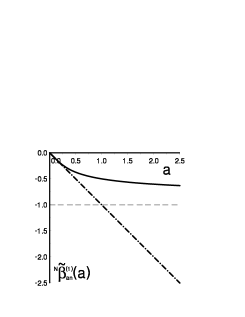
Figure 2: The $\beta$ function corresponding to the one-loop new analytic running coupling (solid curve). The perturbative result is shown as the dot-dashed line.

Figure 2 shows the $\beta$ function (10) and the perturbative result corresponding to the one-loop perturbative running coupling $\widetilde{\alpha}^{(1)}_{\mbox{\scriptsize s}}(q^{2})=1/\ln z$. The $\beta$ function (10) coincides with the perturbative result $\widetilde{\beta}^{(1)}_{\mbox{\scriptsize s}}(a)=-a$ in the region of small values of invariant charge and tends to $-1$ at large $a$. This results in the IR enhancement of the running coupling, namely, $\alpha(q^{2})\sim 1/q^{2}$ when $q^{2}\to 0$. At the higher loop levels the $\beta$ function has the same asymptotics. Thus the NARC possesses the universal IR and UV behavior at any loop level. The $\beta$ function (10) in the region of small $a$ acquires the form ${}^{\mbox{\tiny N}}\!\widetilde{\beta}^{\mbox{\scriptsize(1)}}_{\mbox{\scriptsize an}}(a)=\widetilde{\beta}^{(1)}_{\mbox{\scriptsize s}}(a)+O\left[a^{-1}\exp(-a^{-1})\right]$, which reveals its intrinsically nonperturbative nature. The detailed description of the properties of the NARC can be found in Ref. 8.

4 Applications of the New Analytic Running Coupling

For verification of the consistency of the model proposed one should turn to the applications. Since we are working in the framework of a nonperturbative approach, the study of nonperturbative phenomena is of a primary interest. The most exciting problem here is the quark confinement.

It has been shown $\!{}^{{\bf?},{\bf?}}$ that the new analytic running coupling (7) explicitly leads to the rising at large distances static quark-antiquark potential without invoking any additional assumptions:

$${}^{N}V(r)\sim\frac{8\pi}{3\beta_{0}}\Lambda\,\frac{1}{2}\frac{\Lambda r}{\ln(\Lambda r)},\quad r\to\infty.$$ (11)

For the practical purposes it is worth using the approximating function $U(r)$ for the interquark potential (see Eq. (31) in Ref. 5). The comparison of $U(r)$ with the Cornell phenomenological potential ${}^{C}V(r)=-4a\,/\,(3r)+\sigma r,\,$ $a=0.39,\,$ $\sigma=0.182\,$GeV², as well as with the lattice data $\!{}^{{\bf?}}$ shows their almost complete coincidence.

Figure 3: Comparison of the potential $U(r)$ (solid curve) with the Cornell potential ($\diamond$); $\Lambda=600\,$MeV, $n_{\mbox{\tiny f}}=3$.

Figure 4: Comparison of the potential $U(r)$ (solid curve) with the lattice data ($\diamond$); $\Lambda=580\,$MeV, $n_{\mbox{\tiny f}}=3$.

It should be mentioned here that the normalization $\!{}^{{\bf?}}$ $U(r_{0})=0,\,$ $r_{0}=0.49\,$fm was used, so that $\Lambda_{\mbox{\scriptsize QCD}}$ was the only varied parameter here.

By making use of the one-loop new analytic running coupling the estimation of the parameter $\Lambda_{\mbox{\scriptsize QCD}}$ has been performed recently by calculation of the value of gluon condensate $K\simeq(0.36\,\mbox{GeV})^{4}$. This gave $\Lambda=(650\pm 50)\,$MeV, which is close to the previous estimation.

It turns out that the new analytic running coupling being applied to the standard perturbative phenomena provides the similar values of the parameter $\Lambda$. So, the tentative estimations are the following. The $e^{+}e^{-}\to$ hadrons annihilation gives $\Lambda=490\pm 80\,$MeV, and the $\tau$ lepton decay gives $\Lambda=520\pm 65\,$MeV (light quark mass $m\simeq[2.5\div 6.0]\,$MeV is used here). These values of $\Lambda$ correspond to the one-loop level with three active quarks.

Thus, there is a consistent estimation of the parameter $\Lambda_{\mbox{\scriptsize QCD}}$ in the framework of the approach developed: $\Lambda\simeq 550\,$MeV (one-loop level, $n_{\mbox{\scriptsize f}}=3$). This testifies that the new analytic running coupling combines in a consistent way both nonperturbative and perturbative behavior of QCD.

5 Conclusions

A new model for the QCD analytic running coupling has been proposed.$\!{}^{{\bf?}}$ It was presented explicitly in the renorminvariant form and the relevant $\beta$ function was derived.$\!{}^{{\bf?}}$ The consistent continuation of the NARC to the timelike region is performed.$\!{}^{{\bf?}}$ The NARC possesses a number of appealing features. Namely, there are no unphysical singularities at any loop level. The IR enhancement and the UV asymptotic freedom are incorporated in a single expression. At any loop level the universal IR behavior ($\alpha\sim 1/q^{2}$) is reproduced. The additional parameters are not introduced in the theory. This approach possesses a good loop and scheme stability. The confining static quark-antiquark potential is derived without invoking any additional assumptions.$\!{}^{{\bf?},{\bf?}}$ There is a consistent estimation of the parameter $\Lambda_{\mbox{\scriptsize QCD}}$ in the framework of the current approach. All this implies that the new analytic running coupling substantially incorporates in a consistent way perturbative and nonperturbative behavior of Quantum Chromodynamics.

References

References

- [1] P. J. Redmond, Phys. Rev. 112, 1404 (1958).
- [2] N. N. Bogoliubov, A. A. Logunov, and D. V. Shirkov, Zh. Eksp. Teor. Fiz. 37, 805 (1959) [Sov. Phys. JETP 37, 574 (1960)].
- [3] D. V. Shirkov and I. L. Solovtsov, Phys. Rev. Lett. 79, 1209 (1997); hep-ph/9704333.
- [4] I. L. Solovtsov and D. V. Shirkov, Theor. Math. Phys. 120, 482 (1999); hep-ph/9909305.
- [5] A. V. Nesterenko, Phys. Rev. D 62, 094028 (2000); hep-ph/9912351.
- [6] A. V. Nesterenko, hep-ph/0102124.
- [7] A. I. Alekseev and B. A. Arbuzov, Mod. Phys. Lett. A 13, 1747 (1998); hep-ph/9704228.
- [8] A. V. Nesterenko, Mod. Phys. Lett. A 15, 2401 (2000); hep-ph/0102203.
- [9] A. V. Nesterenko, in Proc. Int. Conf. Confinement IV, Vienna, Austria, 2000, ed. W. Lucha (to be published); hep-ph/0010257.
- [10] G. S. Bali et al., Phys. Rev. D 62, 054503 (2000); hep-lat/0003012.