Rare $B\rightarrow K^{*}\nu\bar{\nu}$ decay with polarized $K^{*}$ in the fourth generation model

The rare $B\rightarrow K^{*}\nu\bar{\nu}$ decay when $K^{*}$ meson is longitudinally or transversely polarized is analysed in the context of the fourth generation model. A significant enhancement to the missing energy spectrum over the SM is recorded.

1 Introduction

The theoretical and experimental investigations of the rare decays has been a subject of continuous interest in the existing literature. The experimental observation of the inclusive $b\rightarrow X_{s}\gamma$ [1], and exclusive $B\rightarrow K^{*}\gamma$ [2] decays, together with the recent CLEO [3] upper limits on the exclusive decays $B\rightarrow K^{*}\ell^{+}\ell^{-}$ which are less than one order of magnitude above the SM predictions, stimulated the study of rare B meson decays on a new footing. These decays take place via flavor-changing neutral currents (FCNC) which are absent in the Standard Model (SM) at tree level and appear only at the loop level. The inclusive $B\rightarrow X_{s}\nu\bar{\nu}$ decay rate is very sensitive to extensions of the SM, and provides a unique source of constrains on some ’new physics’ scenarios which predict a large enhancement of this decay mode. Therefore, the study of $b\rightarrow s\nu\bar{\nu}$, together with the search for $b\rightarrow s\ell^{+}\ell^{-}$, and $b\rightarrow s$ gluon processes, with a refinement of the measurement of $B\rightarrow X_{s}\gamma$ will allow to exploit a complete program to test the SM properties at the loop level and constrain various new physics scenarios. The first attempt to experimentally access the decay $b\rightarrow s\nu\bar{\nu}$ will be through the exclusive modes, which will be better investigated at B-factories. Among such modes, the channel $B\rightarrow K^{*}\nu\bar{\nu}$ provokes special interest. The experimental search for $B\rightarrow K^{*}\nu\bar{\nu}$ decays can be performed through the large missing energy associated with the two neutrinos, together with an opposite side fully reconstructed B meson. The SM has been exploited to establish a bound on the branching ratio of the above-mentioned decay of the order $\sim 10^{-5}$, which can be quite measurable for the upcoming $KEK$ and SLAC B-factories. However, in SM there are three generations, and yet, there is no theoretical argument to explain why there are three and only three generations in SM, and there is neither an experimental evidence for a fourth generation nor does any experiment exclude such extra generations. On this basis, serious attempts to study the effects of the fourth generation on the rare B meson were made by many authors. For examples, the effects of the fourth generation on the branching ratio of the $B\rightarrow X_{s}\ell^{+}\ell^{-}$, and the $B\rightarrow X_{s}\gamma$ decays is analysed in [4]. In [5] the fourth generation effects on the rare exclusive $B\rightarrow K^{*}\ell^{+}\ell^{-}$ decay are studied. In [6] the contributions of the fourth generation to the $B_{s}\rightarrow\nu\bar{\nu}\gamma$ decay is investigated. Recently, in [7] the effects of the fourth generation on the rare $B\rightarrow K^{*}\nu\bar{\nu}$ decay is discussed.

In this work, the missing energy spectrum, and the branching ratio of $B\rightarrow K^{*}\nu\bar{\nu}$ will be investigated when $K^{*}$ meson is longitudinally or transversely polarized in a sequential fourth generation model SM, which we shall call (SM4) hereafter for the sake of simplicity. This model is considered as natural extension of the SM, where the fourth generation model is introduced in the same way the three generations are introduced in the SM, so no new operators appear, and clearly the full operator set is exactly the same as in SM. Hence, the fourth generation will change only the values of the Wilson coefficients via virtual exchange of a up-like quark $\acute{t}$. Subsequently, the missing energy spectrum, and branching ratio of $B\rightarrow K^{*}\nu\bar{\nu}$ are enhanced significantly, as we shall see, a result which is in the right direction at least to help experimental search for $B\rightarrow K^{*}\nu\bar{\nu}$ through $m_{\acute{t}}$, and vice versa.

Consequently, this paper is organized as follows: in Section 2, the relevant effective Hamiltonian for the decay $B\rightarrow K^{*}\nu\bar{\nu}$ in a sequential fourth generation model (SM4) is presented; and in section 3, the dependence of the missing energy spectrum, and branching ratio of $B\rightarrow K^{*}\nu\bar{\nu}$ on the fourth generation model parameters for the decay of interest is studied, when $K^{*}$ meson is longitudinally or transversely polarized using the results of the Light- Cone QCD sum rules for estimating form factors; and finally a brief discussion of the results is given.

2 Effective Hamiltonian

In the Standard Model (SM), the process $B\rightarrow K^{*}\nu\bar{\nu}$ is described at quark level by the $b\rightarrow s\nu\bar{\nu}$ transition, and receives contributions from Z-penguin and box diagrams, where dominant contributions come from intermediate top quarks. The effective Hamiltonian responsible for $b\rightarrow s\nu\bar{\nu}$ decay is described by only one Wilson coefficient, namely $C^{(SM)}_{11}$, and its explicit form is [8]:

$$H_{eff} = \frac{G_{F}\alpha}{2\pi\sqrt{2}sin^{2}\theta_{w}}C^{(SM)}_{11}V^{*}_{ts}V_{tb}\bar{s}\gamma_{\mu}(1-\gamma_{5})b\bar{\nu}\gamma_{\mu}(1-\gamma_{5})\nu,$$ (1)

where $G_{F}$ is the Fermi coupling constant, $\alpha$ is the fine structure constant (at the Z mass scale), and $V^{*}_{ts}V_{tb}$ are products of Cabibbo-Kabayashi-Maskawa matrix elements. In Eq.(1), the Wilson coefficient $C^{(SM)}_{11}$ in the context of the SM has the following form including $O(\alpha_{s})$ corrections [9]:

$$C^{(SM)}_{11}=\left[X_{0}(x_{t})+\frac{\alpha_{s}}{4\pi}X_{1}(x_{t})\right],$$ (2)

with

$$X_{0}(x_{t})=\frac{x_{t}}{8}\left[\frac{x_{t}+2}{x_{t}-1}+\frac{3(x_{t}-2)}{(x_{t}-1)^{2}}ln(x_{t})\right],$$ (3)

where $x_{t}=\frac{m^{2}_{t}}{m^{2}_{W}}$, and

$$X_{1}(x_{t}) = \frac{4x_{t}^{3}-5x_{t}^{2}-23x_{t}}{3(x_{t}-1)^{2}}-\frac{x_{t}^{4}+x_{t}^{3}-11x_{t}^{2}+x_{t}}{(x_{t}-1)^{3}}ln(x_{t})+\frac{x_{t}^{4}-x_{t}^{3}-4x_{t}^{2}-8x_{t}}{2(x_{t}-1)^{3}}ln^{2}(x_{t})$$ (4)

$$+ \frac{x_{t}^{3}-4x_{t}}{(x_{t}-1)^{2}}Li_{2}(1-x_{t})+8x_{t}\frac{\partial X_{0}(x_{t})}{\partial x_{t}}ln(x_{\mu}).$$

Here $Li_{2}(1-x_{t})=\int_{1}^{x_{t}}\frac{lnt}{1-t}dt$ is a specific function, and $x_{\mu}=\frac{\mu^{2}}{m_{w}^{2}}$ with $\mu=O(m_{t})$.

At $\mu=m_{t}$, the QCD correction for $X_{1}(x_{t})$ term is very small (around $\sim 3\%$). From the theoretical point of view, the transition $b\rightarrow s\nu\bar{\nu}$ is a very clean process, since it is practically free from the scale dependence, and free from any long distance effects. In addition, the presence of a single operator governing the inclusive $b\rightarrow s\nu\bar{\nu}$ transition is an appealing property. As has been mentioned in the introduction, no new operators appear, and clearly the full operator set is exactly same as in SM, thus the fourth generation fermion changes only the values of the Wilson coefficients $C^{(SM)}_{11}$ via virtual exchange of the fourth generation up quark $\acute{t}$, i.e:

$$C_{11}^{SM4}(\mu) = C^{(SM)}_{11}(\mu)+\frac{V^{*}_{\acute{t}s}V_{\acute{t}b}}{V^{*}_{tb}V_{ts}}C^{(new)}(\mu),$$ (5)

where $C^{(new)}(\mu)$ can be obtained from $C^{(SM)}_{11}(\mu)$ by substituting $m_{t}\rightarrow m_{\acute{t}}$, and the last terms in these expressions describe the contributions of the $\acute{t}$ quark to the Wilson coefficients. $V_{\acute{t}s}$, and $V_{\acute{t}b}$ are the two corresponding elements of the $4\times 4$ Cabibbo-Kobayashi-Maskawa (CKM) matrix. In deriving Eqs.(5) we factored out the term $V^{*}_{ts}V_{tb}$ in the effective Hamiltonian given in Eq.(1).

As a result, we obtain a modified effective Hamiltonian, which represents $b\rightarrow s\nu\bar{\nu}$ decay in the presence of the fourth generation fermion:

$$H_{eff}=\frac{G_{F}\alpha}{2\pi\sqrt{2}sin^{2}\theta_{w}}V^{*}_{ts}V_{tb}[C_{11}^{(SM4)}]\bar{s}\gamma_{\mu}(1-\gamma_{5})b\bar{\nu}\gamma_{\mu}(1-\gamma_{5})\nu.$$ (6)

However, in spite of such theoretical advantages, it would be a very difficult task to detect the inclusive $b\rightarrow s\nu\bar{\nu}$ decay experimentally, because the final state contains two missing neutrinos and many hadrons. Therefore, only the exclusive channels, namely $B\rightarrow K^{*}(\rho)\nu\bar{\nu}$, are well suited to search for, and constrain for possible ”new physics” effects. In order to compute $B\rightarrow K^{*}\nu\bar{\nu}$ decay, we need the matrix elements of the effective Hamiltonian Eq.(6) between the final, and initial meson states. This problem is related to the non-perturbative sector of QCD, and can be solved only by using non-perturbative methods. The matrix element $<K^{*}\mid H_{eff}\mid B>$ has been investigated in a framework of different approaches, such as chiral perturbation theory [10], three point QCD sum rules [11], relativistic quark model by the light front formalism [12], effective heavy quark theory [13], and light cone QCD sum rules [14,15]. To begin with, let us denote by $P_{B}$, and $P_{K^{*}}$ the four-momentum of the initial and final mesons, and define q=$P_{B}-P_{K^{*}}$ as the four-momentum of the $\nu\bar{\nu}$ pair, and $x\equiv E_{miss}/M_{B}$ the missing energy fraction, which is related to the squared four-momentum transfer $q^{2}$ by: $q^{2}=M^{2}_{B}[2x-1+r^{2}_{K^{*}}]$, where $r_{K^{*}}\equiv M_{K^{*}}/M_{B}$ with $M_{B}$, and $M_{K^{*}}$ being the initial and final meson masses. The hadronic matrix element for the $B\rightarrow K^{*}\nu\bar{\nu}$ can be parameterized in terms of five form factors:

$$<K^{*}_{h}\mid\bar{s}\gamma_{\mu}(1-\gamma_{5})b\mid B>=\frac{2V(q^{2})}{M_{B}+M_{K^{*}}}\epsilon_{\mu\nu\alpha\beta}\epsilon^{*\nu}(h)P_{B}^{\alpha}P^{\beta}_{K^{*}}$$

$$-i\left[\epsilon_{\mu}^{*}(h)(M_{B}+M_{K^{*}})A_{1}(q^{2})-[\epsilon^{*}(h).q](P_{B}+P_{K^{*}})_{\mu}\frac{A_{2}(q^{2})}{M_{B}+M_{K^{*}}}\right.$$

$$-\left.q_{\mu}[\epsilon^{*}(h).q]\frac{2M_{K^{*}}}{q^{2}}[A_{3}(q^{2})-A_{0}(q^{2})]\right],$$ (7)

where $\epsilon(h)$ is the polarization 4-vector of $K^{*}$ meson. The form factor $A_{3}(q^{2})$ can be written as a linear combination of the form factors $A_{1}$ and $A_{2}$:

$$A_{3}(q^{2})=\frac{1}{2M_{K^{*}}}\left[(M_{B}+M_{K^{*}})A_{1}(q^{2})-(M_{B}-M_{K^{*}})A_{2}(q^{2})\right],$$ (8)

with a condition $A_{3}(q^{2}=0)=A_{0}(q^{2}=0)$.

From these form factors it is easy to derive the missing energy distribution corresponding to the helicity $h=0,\pm 1$of the $K^{*}$ meson:

$$\frac{d\Gamma(B\rightarrow K^{*}_{h=0}\nu\bar{\nu})}{dx}=\frac{G_{F}^{2}\alpha^{2}M^{5}_{B}\mid V^{*}_{ts}V_{tb}\mid^{2}}{64\pi^{5}sin^{4}\theta_{w}}\mid C^{SM4}_{11}\mid^{2}\frac{\sqrt{(1-x)^{2}-r^{2}_{K^{*}}}}{r^{2}_{K^{*}}(1+r^{2}_{K^{*}})^{2}}\cdot$$

$$\mid(1+r^{2}_{K^{*}})^{2}(1-x-r^{2}_{K^{*}})A_{1}(q^{2})-2[(1-x)^{2}-r^{2}_{K^{*}}]A_{2}(q^{2})\mid^{2},$$ (9)

$$\frac{d\Gamma(B\rightarrow K^{*}_{h=\pm 1}\nu\bar{\nu})}{dx}=\frac{G_{F}^{2}\alpha^{2}M^{5}_{B}\mid V^{*}_{ts}V_{tb}\mid^{2}}{64\pi^{5}sin^{4}\theta_{w}}\mid C^{SM4}_{11}\mid^{2}\sqrt{(1-x)^{2}-r^{2}_{K^{*}}}\cdot$$

$$\frac{2x-1+r^{2}_{K^{*}}}{(1+r^{2}_{K^{*}})^{2}}\mid 2\sqrt{(1-x)^{2}-r^{2}_{K^{*}}}V(q^{2})\mp(1+r^{2}_{K^{*}})^{2}A_{1}(q^{2})\mid^{2}.$$ (10)

From Eqs.(9,10), we can see that the missing energy spectrum for $B\rightarrow K^{*}\nu\bar{\nu}$ contains three form factors: V, $A_{1}$, and $A_{2}$. In this work, in estimating the missing energy spectrum, we have used the results of [16]:

$$F(q^{2})=\frac{F(0)}{1-a_{F}(q^{2}/M^{2}_{B})+b_{F}(q^{2}/M^{2}_{B})^{2}},$$ (11)

and the relevant values of the form factors at $q^{2}=0$ are:

$$A_{1}^{B\rightarrow K^{*}}(q^{2}=0)=0.34\pm 0.05,{~{}~{}}with{~{}~{}}a_{F}=0.6,{~{}~{}}and{~{}~{}}b_{F}=-0.023,$$ (12)

$$A_{2}^{B\rightarrow K^{*}}(q^{2}=0)=0.28\pm 0.04,{~{}~{}}with{~{}~{}}a_{F}=1.18,{~{}~{}}and{~{}~{}}b_{F}=0.281,$$ (13)

and

$$V^{B\rightarrow K^{*}}(q^{2}=0)=0.46\pm 0.07,{~{}~{}}with{~{}~{}}a_{F}=1.55,{~{}~{}}and{~{}~{}}b_{F}=0.575.$$ (14)

Note that all errors, which come out, are due to the uncertainties of the b-quark mass, the Borel parameter variation, wave functions, and radiative corrections are quadrature added in. Finally, to obtain quantitative results we need the value of the fourth generation CKM matrix elements $V^{*}_{\acute{t}s}V_{\acute{t}b}$. For this aim following [17], we will use the experimental results of the decay $BR(B\rightarrow X_{s}\gamma)$ together with $BR(B\rightarrow X_{c}e\bar{\nu_{e}})$ to determine the fourth generation CKM factor $V^{*}_{\acute{t}s}V_{\acute{t}b}$. However, in order to reduce the uncertainties arising from b-quark mass, we consider the following ratio:

$$R_{quark}=\frac{BR(B\rightarrow X_{s}\gamma)}{BR(B\rightarrow X_{c}e\bar{\nu_{e}})}.$$ (15)

In the leading logarithmic approximation this ratio can be summarized in a compact form as follows [18]:

$$R_{quark}=\frac{\mid V^{*}_{ts}V_{tb}\mid^{2}}{\mid V_{cb}\mid^{2}}\frac{6\alpha}{\pi f(z)}\mid C^{SM4}_{7}(m_{b})\mid^{2},$$ (16)

where

$$f(z)=1-8z+8z^{3}-z^{4}-12z^{2}ln(z){~{}~{}~{}~{}~{}~{}~{}}with{~{}~{}~{}}z=\frac{m^{2}_{c,pole}}{m^{2}_{b,pole}}$$ (17)

is the phase space factor in $BR(B\rightarrow X_{c}e\bar{\nu_{e}})$, and $\alpha=e^{2}/4\pi$. In the case of four generation there is an additional contribution to $B\rightarrow X_{s}\gamma$ from the virtual exchange of the fourth generation up quark $\acute{t}$. The Wilson coefficients of the dipole operators are given by:

$$C^{SM4}_{7,8}(m_{b})=C^{SM}_{7,8}(m_{b})+\frac{V^{*}_{\acute{t}s}V_{\acute{t}b}}{V^{*}_{ts}V_{tb}}C^{new}_{7,8}(m_{b}),$$ (18)

where $C^{new}_{7,8}(m_{b})$ present the contributions of $\acute{t}$ to the Wilson coefficients, and $V^{*}_{\acute{t}s}V_{\acute{t}b}$ are the fourth generation CKM matrix factor which we need now. With these Wilson coefficients and the experiment results of the decays $BR(B\rightarrow X_{s}\gamma)=2.66\times 10^{-4}$, together with the semileptonic $BR(B\rightarrow X_{c}e\bar{\nu_{e}})$=$0.103\pm 0.01$ [19,20] decay, one can obtain the results of the fourth generation CKM factor $V^{*}_{\acute{t}s}V_{\acute{t}b}$, wherein, there exist two cases, a positive, and a negative one [17]:

$$(V^{*}_{\acute{t}s}V_{\acute{t}b})^{\pm}=\biggl{[}\pm\sqrt{\frac{R_{quark}\mid V_{cb}\mid^{2}\pi f(z)}{6\alpha\mid V^{*}_{ts}V_{tb}\mid^{2}}}-C^{(SM)}_{7}(m_{b})\biggr{]}\frac{V^{*}_{ts}V_{tb}}{C^{(new)}_{7}(m_{b})}.$$ (19)

The values for $V^{*}_{\acute{t}s}V_{\acute{t}b}$ are listed in Table 1 [7].

A few comments about the numerical values of $(V^{*}_{\acute{t}s}V_{\acute{t}b})^{\pm}$ are in order. From unitarity condition of the CKM matrix we have

$$V^{*}_{us}V_{ub}+V^{*}_{cs}V_{cb}+V^{*}_{ts}V_{tb}+V^{*}_{\acute{t}s}V_{\acute{t}b}=0.$$ (20)

If the average values of the CKM matrix elements in the SM are used [19], the sum of the first three terms in Eq.(20) is about $7.6\times 10^{-2}$. Substituting the value of $(V^{*}_{\acute{t}s}V_{\acute{t}b})^{(+)}$ from Table 1 [7], we observe that the sum of the four terms on the left-hand side of Eq.(20) is closer to zero compared to the SM case, since $(V^{*}_{\acute{t}s}V_{\acute{t}b})^{(+)}$ is very close to the sum of the first three terms, but with opposite sign. On the other hand if we consider $(V^{*}_{\acute{t}s}V_{\acute{t}b})^{-}$, whose value is about $10^{-3}$, which is one order of magnitude smaller compared to the previous case, and the error in sum of the first three terms in Eq.(20) is about $\pm 0.6\times 10^{-2}$. Therefore, it is easy to see then that, the value of $(V^{*}_{\acute{t}s}V_{\acute{t}b})^{-}$ is within this error range. In summary both $(V^{*}_{\acute{t}s}V_{\acute{t}b})^{+}$, and $(V^{*}_{\acute{t}s}V_{\acute{t}b})^{-}$ satisfy the unitarity condition of CKM, moreover, $\mid(V^{*}_{\acute{t}s}V_{\acute{t}b})\mid^{-}\leq 10^{-1}\times\mid(V^{*}_{\acute{t}s}V_{\acute{t}b})\mid^{+}$. Therefore, from our numerical analysis one cannot escape the conclusion that, the $(V^{*}_{\acute{t}s}V_{\acute{t}b})^{-}$ contribution to the physical quantities should be practically indistinguishable from SM results, and our numerical analysis confirms this expectation. We now go on to put the above points in perspective.

3 Numerical Analysis

In order to investigate the sensitivity of the missing-energy spectra, and branching ratios of rare $B\rightarrow K_{L}^{*}\nu\bar{\nu}$, and $B\rightarrow K_{T}^{*}\nu\bar{\nu}$ decay (where $K_{L}^{*}$, and $K_{T}^{*}$ stand for longitudinally and transversely polarized $K^{*}$-meson, respectively)in SM4, the following values have been used as input parameters:
$G_{F}=1.17{~{}}.10^{-5}~{}GeV^{-2}$, $\alpha=1/137$, $m_{b}=5.0$ GeV, $M_{B}=5.28$ GeV, $\mid V^{*}_{ts}V_{tb}\mid$=0.045, $M_{K^{*}}=0.892$ GeV, and the lifetime is taken as $\tau(B_{d})=1.56\times 10^{-12}$ s [20], also we have run calculations of Eqs.(9,10) adopting the two sets of $(V^{*}_{\acute{t}s}V_{\acute{t}b})^{\pm}$ in Table 1 [7]. we present our numerical results for the missing-energy spectra, and branching ratios in series of graphs. In figures (1-4), we show the missing energy distribution to the decay $dBR(B\rightarrow K_{L}^{*}\nu\bar{\nu})/dx$, and $dBR(B\rightarrow K_{T}^{*}\nu\bar{\nu})/dx$ as functions of $x$; $\frac{1-r^{2}_{K^{*}}}{2}\leq x\leq 1-r_{K^{*}}$, for $m_{\acute{t}}$= 250 GeV, and $m_{\acute{t}}$= 350 GeV. It can be seen their that, when $V^{*}_{\acute{t}s}V_{\acute{t}b}$ takes positive values, i.e. $(V^{*}_{\acute{t}s}V_{\acute{t}b})^{-}$, the missing energy spectrum is almost overlap with that of SM. That is, the results in SM4 are the same as that in SM. But in the second case, when the values of $V^{*}_{\acute{t}s}V_{\acute{t}b}$ are negative, i.e $(V^{*}_{\acute{t}s}V_{\acute{t}b})^{+}$ the curve of the missing energy spectrum is quit different from that of the SM. This can be clearly seen from figures (1-4). The enhancement of the missing energy spectrum increases rapidly, and the missing energy spectrum of the $K^{*}$ meson is almost symmetrical. In figures (5,6), the branching ratio $BR(B\rightarrow K_{L}^{*}\nu\bar{\nu})$, and $BR(B\rightarrow K_{T}^{*}\nu\bar{\nu})$ are depicted as a function of $m_{\acute{t}}$. Figures (5,6) show that for all values of $m_{\acute{t}}\geq 210$ GeV the values of the branching ratios become greater than SM. The enhancement of the branching ratio increases rapidly with the increasing of $m_{\acute{t}}$. In this case, the fourth generation effects are shown clearly. The reason is that $(V^{*}_{\acute{t}s}V_{\acute{t}b})^{+}$ is 2-3 times larger than $V^{*}_{ts}V_{tb}$ so that the last term in Eq.(5) becomes important, and it depends on the $\acute{t}$ mass strongly. Thus the effect of the fourth generation is significant. Whereas, in our approach the predictions for the ratio $B\rightarrow K_{L}^{*}\nu\bar{\nu}/B\rightarrow K_{T}^{*}\nu\bar{\nu}$, as well as the transverse asymmetry $A_{T}$,

$$A_{T}\equiv\frac{Br(B\rightarrow K_{h=-1}^{*}\nu\bar{\nu})-Br(B\rightarrow K_{h=+1}^{*}\nu\bar{\nu})}{Br(B\rightarrow K_{h=-1}^{*}\nu\bar{\nu})+Br(B\rightarrow K_{h=+1}^{*}\nu\bar{\nu})}$$ (21)

are model-independent.

In conclusion, the missing-energy spectra, and branching ratio of rare exclusive semileptonic $B\rightarrow K^{*}\nu\bar{\nu}$ decay has been investigated in the fourth generation model. The effects of possible fourth generation fermion $\acute{t}$ quark mass has been considered, and the sensitivity of the branching ratio, and the missing-energy spectra to $\acute{t}$ quark mass is observed.

Finally, note that the results for $B\rightarrow\rho\nu\bar{\nu}$ decay can be easily obtained from $B\rightarrow K^{*}\nu\bar{\nu}$ when the following replacements are done in all equations: $V_{tb}V^{*}_{ts}\rightarrow V_{tb}V^{*}_{td}$ and $m_{K^{*}}\rightarrow m_{\rho}$. In obtaining these results, one must keep in mind that the values of the form factors for $B\rightarrow\rho$ transition generally differ from that of the $B\rightarrow K^{*}$ transition. However, these differences must be in the range of $SU(3)$ violation, namely in the order $(15-20)\%$.

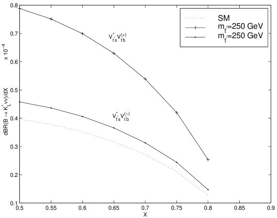
Figure 1:

Figure 2:

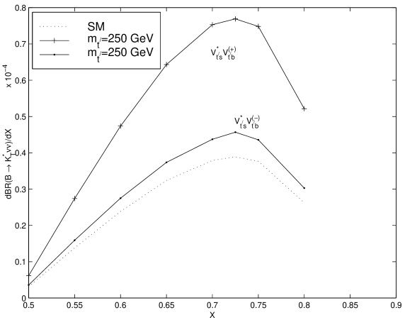
Figure 3:

Figure 4:

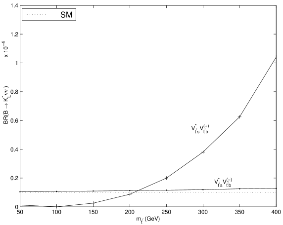
Figure 5:

Figure 6:

References

• [1] M. S. Alam et al., CLEO Collaboration, Phys. Rev. Lett. 74 (1995) 2885.
• [2] R. Ammar et al., CLEO Collaboration, Phys. Rev. Lett. 71 (1993) 674.
• [3] S. Anderson et al., CLEO Collaboration, hep-ex/0106060 (2001).
• [4] C.-S. Huang, W.-J. Huo, and Y.-L. Wu, Mod. Phys. A14 (1999) 2453, [hep-ph/9911203].
• [5] T. M. Aliev, A. $\ddot{O}$zpineci, and M. Savci, Nucl. Phys. B (2000) 275, [hep-ph/0002061].
• [6] Y. DinΓ§er, Phys. Lett. B505, (2001) 89, [hep-ph/0012135].
• [7] T. Barakat, hep-ph/0105116 (2001).
• [8] T. Barakat, J. Phys. G: Nucl.Part. Phys.24 (1998) 1903.
• [9] G. Buchalla, and A. J. Buras, Nucl. Phys. B400 (1993) 225; G. Buchalla, A. J. Buras, and M. E. Lautenbacher, Rev. Mod. Phys. 68 (1996) 1125.
• [10] R. Casalbuoni et al., Phys. Reports 281 (1997) 145.
• [11] P. Colangelo, F. De Fazio, P. Santorelli, and E. Scrimieri, Phys. Rev. D53 (1996) 3672.
• [12] W. Jaus, and D. Wyler, Phys. Rev. D41 (1991) 3405; D. Melikhov, N. Nikitin, and S. Simula, Phys. Lett. B410, (1997) 290, [hep-ph/9704268].
• [13] W. Roberts, Phys. Rev. D54 (1996) 863.
• [14] T. M. Aliev, A. $\ddot{O}$zpineci, and M. Savci, Phys.Rev. D5 (1996) 4260.
• [15] P. Ball, and V. M. Braun, Phys. Rev. D55 (1997) 5561.
• [16] P. Ball, Fermilab-Conf-98/098-T, [hep-ph/9803501]; P. Ball, and V. M. Braun, Phys. Rev. D58 (1998) 094016.
• [17] W.-J. Huo, [hep-ph/0006110].
• [18] A. J. Buras, TUM-hep-316/98, [hep-ph/9806471].
• [19] M. S. Alam, Phys. Rev. Lett. 74 (1995) 2885.
• [20] C. Caso et al., Particle Data Group, Eur.Phys. J. C3 (1998) 1.
Refer to caption