W09 BARYON FORM FACTORS IN QCD

Abstract

This is a summary of perturbative QCD calculations of baryon form factors. For $e^{+}e^{-}$ going to baryon-antibaryon pairs, normalized calculations are available and reported for the entire ground state octet and decuplet, including off-diagonal form factors, and for the $S_{11}$(1535)-$\overline{S}_{11}$. (The latter results are new for this report.) We also include some explanation of how the results come to be.

1 INTRODUCTION

The form factors of baryons have long been studied in electron scattering, and now we are here to discuss new opportunities that can come from an $e^{+}e^{-}$ collider at moderate energies where exclusive cross sections may be measured. One can foresee measurements of the form factors of baryons in the timelike region. The richness of these measurements should be clear. We can in principle measure the elastic and transition form factors of any baryon, since the baryon-antibaryon pair is produced in the reaction. We are not limited to baryons which exist in stable targets.

This talk will focus on results obtained using perturbative QCD (pQCD). They will therefore be valid at high $Q^{2}$, but should at a minimum serve as an estimate of which form factors will be big and which will be small. It should be emphasized that pQCD is not a model. It is an outcome of the real theory of the strong interactions. The scaling laws can be quoted and demonstrated without approximation, and normalized calculations proceed directly if the lowest Fock state wave functions of the quarks inside the hadrons are known. Some modeling is, however, needed for the latter. The models are not pure invention, since significant information about (moments of, at least) the wave functions can be gotten from QCD sum rule calculations and, less extensively, from lattice gauge theory.

We will tabulate and discuss the results for the form factors, elastic and non-elastic, for the entire ground state baryon octet and decuplet in the third section. The results are taken from many places in known literature. We will also give some new results for form factors involving the $S_{11}$(1535), where it happens that the ingredients have been available for some time, but had been put together for nucleon to $S_{11}$ transitions but not for the elastic case.

The second section will contain a brief summary of how the results come to be, including some necessary special attention to the peculiar case of the nucleon to $\Delta$(1232) transition form factor.

2 HOW TO DO IT

2.1 Basics

At high $Q^{2}$, the magnetic form factor $G_{M}$ (but not the electric one $G_{E}$) can be calculated using perturbative QCD. The basic result is that the form factor factors into terms representing the wave function or distribution amplitude of the baryons and a hard scattering kernel. Schematically,

$$G_{M}=\int[dx][dy]\Phi(y,Q^{2})T_{H}(x,y,Q^{2})\Phi(x,Q^{2})\ .$$ (1)

In more detail, the lowest Fock component of a proton can be represented as [1]

$$|p,\uparrow\rangle = \int{[dx\,d^{2}k_{T}]\over(x_{1}x_{2}x_{3})^{1/2}}$$

$$\times \Big{\{}{\psi_{S}(x_{i},k_{iT})\over\sqrt{6}}\left(2udu-uud-duu\right)_{\uparrow\downarrow\uparrow}$$

$$+ \quad{\psi_{A}(x_{i},k_{iT})\over\sqrt{2}}\left(uud-duu\right)_{\uparrow\downarrow\uparrow}\Big{\}}\ .$$

There are two lowest Fock wave functions for isospin 1/2 particles like the nucleons, $\psi_{S,A}$. If $k_{T}$ is limited and if $Q>>\langle k_{T}\rangle$, one can get the factored $G_{M}$, using

$$\phi_{S,A}(x,Q^{2})=\int^{\sim Q}[d^{2}k_{T}]\psi_{S,A}(x,k_{T})$$ (3)

where one expects the $Q$ dependence to be quite weak, and results like

$$G_{M} = {1\over Q^{4}}\left(16\pi\alpha_{s}\over 3\right)^{2}\int[dx\,dy]\times\Big{\{}2T_{1}\phi_{S}(x)\phi_{S}(y)$$ (4)

$$+ {2\over 3}(T_{1}+2T_{2})\phi_{A}(x)\phi_{A}(y)+{\rm cross\ terms}\Big{\}}.$$

Here, the $1/Q^{4}$ and $T_{1,2}$ have come from evaluating the hard scattering kernel, and [1, 2]

$$T_{2}={1\over x_{1}x_{3}(1-x_{1})y_{1}y_{3}(1-y_{3})}\ ,$$ (5)

and similarly for $T_{1}$.

2.2 Scaling and spin rules

This section could be subtitled “Properties of the hard scattering kernel.” There are scaling and spin selection rules that follow simply from a few precepts. A typical diagram for $T_{H}$ is shown in Fig. 1.

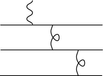
Figure 1: Example of lowest order perturbation theory diagram hard scattering kernel in baryon form factor calculation.

To get the power of $Q$ associated with this diagram, the rules are

• $1/Q^{2}$ for each gluon propagator,

• $1/Q$ for each quark propagator,

• Q for each quark line.

The spin selection rules are (in part),

• quark helicity is conserved,

• if a single gluon or photon is connected to a quark line, it must have transverse polarization,

• if two vector bosons are attached to a quark line, one must have transverse polarization, the other must have longitudinal polarization,

• the helicities of two quarks connected by a transverse gluon must be opposite.

There are also definitional $Q$’s. The above rules are for Feynman diagrams, and a form factor may be defined as a certain factor times a basic matrix element.

Any of the rules can be violated, but it “costs” factors of $O(m/Q)$ or of $O(\langle k_{T}\rangle/Q)$

2.3 Application to nucleon

For the nucleon, in the Breit frame one can show

$$G_{M} \equiv {1\over Q\sqrt{2}}\langle p,\uparrow|\varepsilon_{T}\cdot J|p,\uparrow\rangle$$ (6)

$$\propto {1\over Q}\times{1\over Q^{3}}={1\over Q^{4}}$$

where $\varepsilon$ is a photon polarization vector, $J$ is the electromagnetic current operator, and the arrows are for helicity in the Breit frame. Further,

$$G_{E}\equiv {1\over 2m_{N}}\langle p,\downarrow|\varepsilon_{T}\cdot J|p,\uparrow\rangle$$

$$\propto {\langle k_{T}\rangle\over Q}\times{1\over Q^{3}}={1\over Q^{4}}$$ (7)

For $G_{M}$, an extra $1/Q$ comes from its definition, but for $G_{E}$ the extra $1/Q$ is due to violating a spin selection rule. The predicted falloff famously works well for $G_{M}$, beginning at $Q^{2}$ below 10 GeV².

The results can also be converted into Dirac and Pauli form factors,

$$F_{1} = {\tau G_{M}+G_{E}\over\tau+1}$$

$$F_{2} = {G_{M}-G_{E}\over\tau+1}\propto{1/Q^{6}},{\rm at\ high\ }Q^{2},$$ (8)

where $\tau=Q^{2}/4m_{N}^{2}$. Note that $G_{M}$ and $F_{1}$ become identical at high $Q^{2}$. The prediction for $F_{2}$ is not yet working well [3].

2.4 Other Resonances

This section will be mainly about notation, with numerical results coming later. Electromagnetic nucleon to resonance transitions are often, as in the tables of the Particle Data Group, given in terms of scaled helicity amplitudes—$A_{1/2}$ and $A_{3/2}$ for photons with transverse polarization. For convenience in writing cross section formulas, these amplitude have been divided by the momentum of the photon causing the transition, in the real photon limit. This momentum is zero for an elastic form factor, so the the $A_{1/2,3/2}$ notation is useless for elastic transitions. I feel it is better to always use an unscaled helicity form factor. With a mass factor inserted to make the form factor dimensionless, one has [4]

$$2m_{N}G_{+}=\langle B^{\prime},+{1\over 2}|\varepsilon_{T}\cdot J|B,+{1\over 2}\rangle$$ (9)

where the $+1/2$ is in both cases a helicity in the Breit frame. (Equivalent is the $f_{+}$ from [5], with $2m_{N}G_{+}=\sqrt{2m_{B}^{\prime}2m_{B}}f_{+}$.) Using $G_{+}$ one can directly compare elastic and off-diagonal form factors. Useful connections are

$$G_{M}={m_{N}\sqrt{2}\over Q}G_{+}(N\rightarrow N)$$

$$A_{1/2}=e\sqrt{m_{N}\over m_{R}^{2}-m_{N}^{2}}G_{+}(N\rightarrow R).$$ (10)

(where $e$ is the electric charge). It is also possible to define $F_{1}$ in a straightforward manner, asymptotically as $(m_{N}\sqrt{2}/Q)G_{+}$, for off-diagonal transitions and use it to make interbaryon comparisons.

Stoler has presented plots testing the pQCD scaling for nucleon to resonance transitions [6]. The scaling predicted by perturbative QCD works for three cases out of four, starting safely below 10 GeV² and continuing until the data runs out just past 20 GeV². The exception is the $N\rightarrow\Delta$(1232) transition, which will get a dedicated discussion in the next section.

2.5 The Distribution Amplitudes

This will be just a brief description of how one uses QCD sum rules to get distribution amplitudes for resonances. A full description can be gotten from the original literature [7, 8], or from lectures written up by the present author [9] (who was among those who extended the method to the Delta resonance [10]).

The idea is to start with some function, such as,

$$I(q)=i\int d^{4}ye^{-iqy}\ \langle 0|TO_{1}(y)\ O_{2}(0)|0\rangle$$ (11)

that one can evaluate in two different ways. Before doing any evaluation, however, one chooses at least one of the operators to ensure that only intermediate states of the desired quantum numbers (e.g., isospin 3/2, positive parity, if one is interested in the Delta) can enter.

One of the ways to evaluate is a quark/gluon evaluation, which will depend on already fitted parameters like the density of quark pairs and gluons in the physical vacuum, but which can be evaluated from start to finish. The other way is a purely hadronic evaluation, done by inserting complete sets of intermediate states between the two operators, which depends on the wave functions of the quarks inside the hadron. One actually gets moments of the distribution amplitude (the distribution amplitude multiplied by powers of momentum fractions, and integrated), the moment depending on the details of the operator chosen. Then one matches the two results to get the numerical value of the moment.

Having all the moments is equivalent to having the wave function. Unfortunately, uncertainties in the evaluations build up for higher moments, so that one only gets a few low moments. The information is still valuable, and allows reasonable and normalized choices for distribution amplitudes of the various particles. Uncertainties also build up for any state but the lowest in a given category. For example, in the non-strange sector, results are only available for the nucleon, the Delta(1232), and the $S_{11}$(1535). The results for the moments generally show an asymmetric distribution amplitude for the octet baryons, wherein quarks with helicity paralleling the parent baryon generally carry a larger that equipartition share of the momentum. The distribution amplitudes for the decuplet is, on the other hand, rather symmetrical with momenta on the average evenly divided.

3 NUMERICAL PREDICTIONS

3.1 Nucleon Form Factors

We can be brief. For the nucleon form factors, in the spacelike region, the data has long been known. Hence the data is well fit by the theory—or else we would never of heard of the theory.

There are criticisms of the use of pQCD at current experimental momentum transfers. We will hardly discuss these here. They are based on excising contributions where internal four-momenta squared are low, and seeing what remains. In my opinion, the cutoffs used are quite pessimistic, and further do not consider that internal lines with low four-momentum squared can be quite perturbative if they are short range in coordinate space. Discussion on the positive side can be found in [11], and on the negative side in [12].

3.2 The Nucleon $\rightarrow$ Delta

The pQCD scaling is not seen for the $N\rightarrow\Delta$(1232) electromagnetic transition. Instead we have the DDR—the Disappearing Delta Resonance, and the resonance peak sinks into the background with increasing $Q^{2}$.

But we now know the distribution amplitudes $\phi_{\Delta}$ and $\phi_{S,A}$ for the nucleon, and [13]

$$m_{N}Q^{3}G_{+}(N\rightarrow\Delta)=\left(16\pi\alpha_{s}^{2}/9\right)^{2}\times\qquad\qquad$$

$$\times\left\{{2\over 3}\langle\phi_{A}|T_{1}-T_{2}|\phi_{S}\rangle+{1\over\sqrt{3}}\langle\phi_{A}|T_{1}|\phi_{A}\rangle\right\}$$ (12)

There is a substantial cancellation between the two terms above. The numbers are,

$$Q^{3}G_{+}(N\rightarrow\Delta)=\left\{\begin{array}[]{cl}0.05{\rm GeV}^{3}&\quad{\rm CZ,CP}\\ 0.08{\rm GeV}^{3}&\quad{\rm KS,CP}\\ 0.02{\rm GeV}^{3}&\quad{\rm COZ,FZOZ\,,}\end{array}\right.$$ (13)

where the letter codes refer to distribution amplitudes for the nucleon and Delta, in that order, from papers in [7, 8, 10, 14, 15, 16].

The numbers are small. For comparison,

$$Q^{3}G_{+}(p\rightarrow p)={1\over m_{N}\sqrt{2}}Q^{4}G_{M}\approx 0.75{\rm\ GeV}^{3},$$ (14)

and

$$Q^{3}G_{+}(p\rightarrow N^{*}(1535))=\left\{\begin{array}[]{cl}0.46{\rm GeV}^{3}&\quad{\rm CZ,CP}\\ 0.58{\rm GeV}^{3}&\quad{\rm KS,CP\,.}\end{array}\right.$$ (15)

We conclude that, in distinction to the situation for other form factors, the leading order $N\rightarrow\Delta$ form factors are not currently above background. There is a corollary, which is that the spin prediction $E_{1+}=M_{1+}$ for $Q\rightarrow\infty$ is no seen because the leading order amplitude is not yet dominant. We expect, or hope, that $Q^{2}>10GeV^{2}$ will show some noticeable leading order amplitude, with the ratio $E_{1+}/M_{1+}$ rising. There is further discussion in [17, 18].

3.3 Other Baryons

We come finally to present the results for a whole array of baryons. These predictions depend on distribution amplitudes obtained from QCD sum rules in [10, 16, 15, 14], with special credit gong to the last listed for having done the largest number of baryon resonances.

We quote in all cases values for $Q^{4}F_{1}$ in GeV⁴, calculated with a fixed $\alpha_{s}=0.3$. First in Table 1, we give $Q^{4}F_{1}$ for diagonal transitions (e.g., $\Sigma^{+}$ for the timelike region means $\Sigma^{+}\overline{\Sigma^{+}}$ = $\Sigma^{+}\overline{\Sigma}^{-}$) for the ground state baryon octet. The prediction for the $\Sigma^{0}\rightarrow\Lambda^{0}$ electromagnetictransition is also given. (For full set of octet baryons, there are also predictions from the diquark model [19].)

octet baryon	$Q^{4}F_{1}$ GeV4
n	$-$0.5
p	1.0
$\Sigma^{-}$	$-$0.65
$\Sigma^{0}$	0.27
$\Sigma^{+}$	1.19
$\Lambda^{0}$	$-$0.23
$\Xi^{-}$	$-$0.60
$\Xi^{0}$	$-$0.52
$\Sigma^{0}\rightarrow\Lambda^{0}$	0.54

Table 1: Asymptotic form factors $F_{1}$ for the octet baryons.

Table 2 is the same but for the ground state decuplet baryons. These tend to be smaller than the octet because the smoothness of the wave function gives less strength near the end points, where the bulk of the contributions arise.

decuplet baryon	$Q^{4}F_{1}$ GeV4
$\Omega$	$-$0.02
$\Xi^{*-}$	$-$0.083
$\Xi^{*0}$	0.014
$\Sigma^{*-}$	$-$0.031
$\Sigma^{*0}$	0.016
$\Sigma^{*+}$	0.062
$\Delta^{-}$	$-$0.085
$\Delta^{0}$	0
$\Delta^{+}$	0.085
$\Delta^{++}$	0.17

Table 2: Asymptotic form factors $F_{1}$ for the decuplet baryons.

And then in table 3 we have $Q^{4}F_{1}$ for the ground state decuplet to octet baryon transitions, or associated baryon-antibaryon production in the timelike region.

octet-decuplet transition	$Q^{4}F_{1}$ GeV4
n $\rightarrow\Delta^{0}$	$-$0.08
p $\rightarrow\Delta^{+}$	0.08
$\Sigma^{-}\rightarrow\Sigma^{*-}$	0.016
$\Sigma^{0}\rightarrow\Sigma^{*0}$	0.024
$\Sigma^{+}\rightarrow\Sigma^{*+}$	0.033
$\Lambda^{0}\rightarrow\Sigma^{*0}$	0.015
$\Xi^{-}\rightarrow\Xi^{*-}$	0.013
$\Xi^{0}\rightarrow\Xi^{*0}$	0.024

Table 3: Asymptotic form factor $F_{1}$ for the octet to decuplet baryon transitions.

Finally, we have table 4 which gives the asymptotic $Q^{4}F_{1}$ for transitions involving the negative parity $S_{11}$(1535) resonance. A surprise is the large size of the neutral $S_{11}$ elastic form factor.

transition	$Q^{4}F_{1}$ GeV4
n $\rightarrow S_{11}^{0}$	0.35
p $\rightarrow S_{11}^{+}$	0.7
$S_{11}^{0}\rightarrow S_{11}^{0}$	1.6
$S_{11}^{+}\rightarrow S_{11}^{+}$	0.17

Table 4: Asymptotic form factors $F_{1}$ for transitions involving the $S_{11}$(1535).

3.4 Comments on $e^{+}e^{-}\rightarrow B\bar{B}$

As is too commonly said, the relation between the spacelike and timelike region at finite $Q^{2}$ requires more thought. The data [20] on $F_{1}$ or $G_{M}$ for $p\bar{p}$ is about twice as large at timelike $Q^{2}$ than at the corresponding spacelike $Q^{2}$ in the 10 GeV² region. A rough estimate of the effects of quark mass and transverse momenta shows that a factor of 2 in this $Q^{2}$ region in reasonable from the theoretical side. (The estimate is along the lines of estimates in the spacelike region showing that the mass term in the dipole parameterization of about 0.71 GeV² is reasonable [21].) One can take several attitudes to this statement. One is that pQCD with expected amendations does well. Another is that is shows that we are not at the point where masses are neglectable. These are higher twist effects, and there are others, including contributions of higher Fock states to the form factors.

4 LAST THOUGHTS

Baryon form factors are calculable at high $Q^{2}$ using perturbative QCD in either the spacelike or timelike region. The results are experimentally good for the nucleon elastic and nucleon to $S_{11}$ form factors at $Q^{2}$ above a few GeV² spacelike, and one can explain the lack of currently observed scaling of the nucleon to $\Delta$(1232) transition.

The proposed $e^{+}e^{-}$ machine is a vehicle to measure timelike form factors for a host of unstable baryons. Predictions exist to shoot at for octet elastic, decuplet elastic, octet-decuplet off-diagonal, and $S_{11}$ form factors. There are also non-pQCD predictions, for example those reported by Dubnicka et al. at this meeting [22], and prediction from the diquark model by Jakob et al [19].

The results will cast light on the quarkic wave functions of baryons. The predictions quoted here are specific to the QCD sum rule wave functions we have used. The actual wave functions may be different and the form factor measurements, with the possibility of combining them with $J/\psi,\psi,\ldots\rightarrow B\bar{B}$ and $\gamma\gamma\rightarrow B\bar{B}$, can help ferret them out.

References

- [1] G. P. Lepage and S. J. Brodsky, Phys. Rev. D 22, 2157 (1980).
- [2] V. L. Chernyak and A. R. Zhitnitsky, Sov. J. Nucl. Phys. 31 (1980) 544 [Yad. Fiz. 31 (1980) 1053].
- [3] M. K. Jones et al. [Jefferson Lab Hall A Collaboration], Phys. Rev. Lett. 84, 1398 (2000) [nucl-ex/9910005].
- [4] C. E. Carlson, Phys. Rev. D 34, 2704 (1986).
- [5] J. D. Bjorken and J. D. Walecka, Annals Phys. 38 (1966) 35.
- [6] P. Stoler, Phys. Rev. D 44 (1991) 73.
- [7] V. L. Chernyak and I. R. Zhitnitsky, Nucl. Phys. B 246, 52 (1984).
- [8] I. D. King and C. T. Sachrajda, Nucl. Phys. B 279, 785 (1987).
- [9] C. E. Carlson, in Nucleon Resonances and Nucleon Structure, ed. G. A. Miller, pp. 105 (World Scientific, Singapore, 1992); also in Int. Jour. Mod. Phys. E 1, 525 (1992).
- [10] C. E. Carlson and J. L. Poor, Phys. Rev. D 38, 2758 (1988).
- [11] C. Ji, A. F. Sill and R. M. Lombard, Phys. Rev. D 36, 165 (1987); H. Li and G. Sterman, Nucl. Phys. B 381, 129 (1992).
- [12] N. Isgur and C. H. Llewellyn Smith, Nucl. Phys. B 317, 526 (1989); J. Bolz, R. Jakob, P. Kroll, M. Bergmann and N. G. Stefanis, Z. Phys. C 66, 267 (1995) [hep-ph/9405340].
- [13] C. E. Carlson, M. Gari and N. G. Stefanis, Phys. Rev. Lett. 58, 1308 (1987).
- [14] V. L. Chernyak, A. A. Ogloblin and I. R. Zhitnitsky, Z. Phys. C 42 (1989) 583 [Yad. Fiz. 48 (1989) 1398]; V. L. Chernyak, A. A. Ogloblin and I. R. Zhitnitsky, Z. Phys. C 42, 569 (1989) [Yad. Fiz. 48, 1410 (1989)].
- [15] G. R. Farrar, H. Zhang, A. A. Ogloblin and I. R. Zhitnitsky, Nucl. Phys. B 311, 585 (1989).
- [16] J. Bonekamp and W. Pfeil, Bonn report (1989).
- [17] C. E. Carlson and N. C. Mukhopadhyay, Phys. Rev. Lett. 81, 2646 (1998) [hep-ph/9804356].
- [18] C. E. Carlson and C. R. Ji, in preparation.
- [19] R. Jakob, P. Kroll, M. Schurmann and W. Schweiger, Z. Phys. A 347, 109 (1993) [hep-ph/9310227]; see also P. Kroll, T. Pilsner, M. Schurmann and W. Schweiger, Phys. Lett. B 316, 546 (1993) [hep-ph/9305251].
- [20] M. Ambrogiani et al. [E835 Collaboration], Phys. Rev. D 60, 032002 (1999).
- [21] S. J. Brodsky and B. T. Chertok, Phys. Rev. D 14, 3003 (1976).
- [22] Also in R. Baldini, E. Pasqualucci, S. Dubnicka, P. Gauzzi, S. Pacetti and Y. Srivastava, Nucl. Phys. A 666 (2000) 38; and hep-ph/0106006.