Out-of-plane QCD radiation
in hadronic $Z_{0}$ production

Abstract:

We present the QCD analysis of the cumulative out-of-event-plane momentum distribution in the process $p{\bar{p}}$ into $Z_{0}$ and a hard jet (event plane defined by the $p{\bar{p}}$ and $Z_{0}$ momenta). Particular attention is placed on the near-to-planar events for which we derive the all-order resummed result to next-to-leading accuracy. We consider also the leading power correction originating from the fact that, even in hard processes, the resummed QCD coupling runs into the infrared region. We aim at the same level of accuracy which, in $e^{+}e^{-}$ annihilation, seems to be sufficient for making predictions. Contributions from a “soft underlying event” due to beam remnant interactions are discussed. Experimental data (not yet available) are needed to cast light on the predictive level of standard QCD analysis in hard hadron-hadron collisions. We plot examples of the predicted distribution at Tevatron energies. The techniques here developed can be extended to other hard hadron-hadron and hadron-lepton processes.

1 Introduction

QCD radiation (jet shape distributions) in $e^{+}e^{-}$ annihilation has been intensively studied at the accuracy needed to make quantitative predictions [1]–[8] (double and single logarithmic resummations, matching with fixed order exact results and power suppressed corrections). These distributions have provided various tests of QCD [9] and measurements of the running coupling [10].

For hard hadron-hadron (hh) collisions, the analysis of the associated QCD radiation is more complex than in $e^{+}e^{-}$ annihilation. There are three main differences between the two processes. First, the analyzed $e^{+}e^{-}$ jet-shape distributions are collinear and infrared safe (CIS) quantities (all soft and collinear divergences cancel). On the contrary, in hard hh-collisions [11], jet-shape distributions are finite only after factorizing collinear singular contributions from initial state radiation (giving rise to incoming parton distributions at the appropriate hard scale).

A second important difference between the two processes is that, while in hard hh-collisions a typical event is a multi-jet emission (originating from two incoming partons and from partons going out from the hard elementary collision), in $e^{+}e^{-}$ annihilation the bulk of events is given by $2$-jet emission (originating from the primary $q\bar{q}$ pair). Only recently have $3$-jet event shape $e^{+}e^{-}$ observables been studied: the thrust minor $T_{m}$ [2] and the $D$-parameter [3] in the near to planar $3$-jet limit and the light-jet mass and narrow-jet broadening [12, 13] in the $2$-jet limit. In this paper we are mainly interested in the near to planar $3$-jet limit.

Finally, in hard hh-collisions the standard QCD description does not account for the entire emitted radiation. One needs to add a soft underlying event, not present in $e^{+}e^{-}$ annihilation, which could be considered to result from low-$p_{t}$ interactions involving the spectator partons (beam remnant interaction). The necessity of adding such a component to the radiation was studied in [14], in which was analysed the “pedestal height” in hard jet production, i.e. the mean transverse energy per unit rapidity accompanying a high-transverse-energy jet. The pedestal height and its jet transverse energy dependence measured at the CERN $p\bar{p}$ collider [15] are accounted for by superimposing on the standard hard QCD emission a soft underlying event similar to that of a minimum-bias collision. For more recent analysis on the features of the beam remnant interaction see [16].

In this paper we consider the process

$$h_{1}+h_{2}\to Z_{0}\>+\>\mbox{jet}+\ldots$$ (1)

with $h_{1},h_{2}$ the two incoming hadrons (where $h_{1}h_{2}$ are $pp$ or $p\bar{p}$). The weak $Z_{0}$ boson is emitted with large transverse momentum $Q_{t}$. Here the dots represent initial state jets and intra-jet hadrons. Defining the event plane as the plane formed by the $h_{1},h_{2}$ and $Z_{0}$ momenta, we consider the distribution in the observable $K_{\mbox{\scriptsize out}}$ defined as

$$K_{\mbox{\scriptsize out}}={\sum_{h}}^{\prime}\,|{p_{h}^{\mbox{\scriptsize out}}}|\>,$$ (2)

where $p_{h}^{\mbox{\scriptsize out}}$ is the out-of-plane momentum of the hadron $h$. To avoid measurements in the beam regions, the sum indicated by $\sum_{h}^{\prime}$ extends over all hadrons not in the beam direction, i.e. emitted outside a cone around the beams.

The process (1) involves three jets: the large angle jet (generated by the hard parton recoiling against the weak boson) and the two initial state jets (generated by the incoming partons). The observable $K_{\mbox{\scriptsize out}}$ is similar to $T_{m}$, the $3$-jet shape observable in $e^{+}e^{-}$ annihilation, in which the event plane is defined by the thrust and the thrust major axes. Our analysis of $K_{\mbox{\scriptsize out}}$ will then make use of the methods introduced for the study of $T_{m}$ [2]. We will obtain the following factorized perturbative (PT) contributions and $1/Q_{t}$ power corrections:

• incoming parton distributions at the proper hard scale. They will be obtained from resummations of all powers $\alpha_{\mbox{\scriptsize s}}^{n}\ln^{n}\mu/K_{\mbox{\scriptsize out}}$ ($\mu$ is the small factorization scale needed to subtract the collinear singularities and, as we shall see, $K_{\mbox{\scriptsize out}}$ is the hard scale for these distributions);

• “radiation factors” characteristic of our observable. They will be obtained, for small $K_{\mbox{\scriptsize out}}$, from resummations of double logarithmic (DL) and single logarithmic (SL) terms ($\alpha_{\mbox{\scriptsize s}}^{n}\ln^{n+1}K_{\mbox{\scriptsize out}}/Q_{t}$ and $\alpha_{\mbox{\scriptsize s}}^{n}\ln^{n}K_{\mbox{\scriptsize out}}/Q_{t}$ respectively). From the collinear contributions we need to exclude the pieces already accounted for by the reconstruction of the hard scale $K_{\mbox{\scriptsize out}}$ in incoming parton distributions. As we shall see, the hard scales in the radiation factor, of order $Q_{t}$, are determined by the geometry of the hard elementary process. To identify the scales to this accuracy we need to work at the SL level;

• matching of the above resummed result with the fixed order exact calculations. This allows us to obtain a description of the distribution in the full range of $K_{\mbox{\scriptsize out}}$ (small or of order $Q_{t}$);

• leading $1/Q_{t}$–power corrections to the PT result for the radiation factor. The incoming parton factor has corrections which are of second order ($1/Q_{t}^{2}$), see [5], and they will not be considered here.

The first three points belong to standard PT analysis. Concerning the last point, these non-perturbative (NP) corrections originate from the fact that, resumming the PT expansion, one reconstructs the running coupling $\alpha_{\mbox{\scriptsize s}}(k_{t})$ at the virtual scale which assumes values between $k_{t}\sim Q_{t}$ and $k_{t}=0$. They should not be confused with soft underlying event contributions due to beam remnant interaction, which will be considered later.

To deal with the running coupling in the small $k_{t}$ region we use the same procedure followed in the analysis of $e^{+}e^{-}$ jet-shape distributions. We extrapolate the running coupling into the large distance region using the dispersive approach [5] and we determine the coefficient of $1/Q_{t}$ corrections in terms of a single parameter, usually denoted by $\alpha_{0}$, which is given by the integral of the QCD coupling over the region of small momenta $k\leq\mu_{I}$ (the infrared scale $\mu_{I}$ is conventionally chosen to be $\mu_{I}=2\mathop{\rm Ge\!V}$, but the results are independent of its specific value). Effects of the non-inclusiveness of $K_{\mbox{\scriptsize out}}$ will be included by taking into account the Milan factor ${\cal{M}}$ introduced in [6] and analytically computed in [7]. The NP parameter $\alpha_{0}$, which is the same for all jet shape observables linear in the transverse momentum of emitted hadrons, has been measured and appears to be universal with a reasonable accuracy [9].

There are a number of differences between the analysis of $K_{\mbox{\scriptsize out}}$ in the hh-process (1) and that of $T_{m}$ in $e^{+}e^{-}$ annihilation, besides that concerning initial state radiation mentioned above. First of all in the present case the event plane is defined by the $h_{1},h_{2},Z_{0}$ momenta while in $e^{+}e^{-}$ it is defined by the full structure of the emitted radiation. Then in $e^{+}e^{-}$ one has a complicated interplay between the observable and the event plane definition (technically one has to introduce various Fourier integration variables needed to factorize the event plane condition). These complications are absent in the present case. A second important difference is the presence of the recoil momenta of partons underlying the three jets. The recoil components enter the observable, the kinematics and the matrix element. In the $e^{+}e^{-}$ case all three primary partons generating the jets move out of the event plane, due to the recoil with the emitted secondary partons. In the present case, instead, the two incoming partons (at a low subtraction scale) are fixed along the beam direction by the kinematics of the parton process. This makes relevant the presence of the rapidity cut excluding the beam region (see later).

The paper is organized as follows. In section 2 we define the process under consideration, the observable $K_{\mbox{\scriptsize out}}$ and its distribution. We specify the phase space region of $K_{\mbox{\scriptsize out}}$ in which we perform the QCD study. In section 3 we introduce the factorized structure of the distribution at parton level: the hard elementary partonic process, incoming parton distributions at the hard scale and radiation factor corresponding to our observable. In section 4 we perform the resummation at SL accuracy (we start from the analysis of soft contributions). We show here how to factorize the two contributions generating the incoming parton distributions and the radiation factor. In section 5 we obtain the PT contribution to the radiation factor and its NP correction. In section 6 we compute the distribution, matched to the exact fixed-order result, and we present some numerical results. Finally, section 7 contains a summary, discussions and conclusions. We add few technical Appendices A-F. In the last one (Appendix G) we discuss the contribution of beam remnant interaction.

2 The process and the observable

The incoming hadrons and $Z_{0}$ momenta in the process (1) are given by

$$h_{1}=\mbox{\small$\frac{1}{2}$}\sqrt{s}\,(1,0,0,1)\>,\quad h_{2}=\mbox{\small$\frac{1}{2}$}\sqrt{s}\,(1,0,0,-1)\>,\quad Q=(Q_{0},0,Q_{t},Q_{z})\>,$$ (3)

with large $Q_{t}$ of order of the $Z_{0}$ mass $M$. The $Z_{0}$ is taken on-shell, and its decay products are excluded from our calculation. Including the hadronic decays is possible by following the analysis of $2$-jet emission in $e^{+}e^{-}$ annihilation. The observable $K_{\mbox{\scriptsize out}}$ is given by (2) where $p_{h}^{\mbox{\scriptsize out}}=p_{hx}$, since the event plane is the $yz$-plane, and the sum extends over all hadrons with rapidity $\eta_{h}$ in the range

$$|\eta_{h}|<\eta_{0}\simeq-\ln\tan\frac{\Theta_{0}}{2}\>,$$ (4)

with $\eta_{0}$ large. This implements a cut of angle $\Theta_{0}$ around the two beam directions. To avoid a strong dependence on $\eta_{0}$ we will consider $K_{\mbox{\scriptsize out}}$ not too small (see later).

We study the integrated distribution in $K_{\mbox{\scriptsize out}}$ at fixed $Q_{t}$:

$$\begin{split}\frac{d\sigma(K_{\mbox{\scriptsize out}})}{dQ_{t}}=\sum_{m}\int\frac{d\sigma_{m}}{dQ_{t}}\>\Theta\left(K_{\mbox{\scriptsize out}}-\sum_{h=1}^{m}{}^{\prime}|p_{hx}|\right)\>,\end{split}$$ (5)

with $d\sigma_{m}/dQ_{t}$ the differential distribution for $m$ emitted hadrons in the process under consideration. We then use this to analyse the normalized $K_{\mbox{\scriptsize out}}$ distribution for events with the $Z_{0}$ transverse momentum greater than some cut-off $Q_{m}$:

$$\begin{split}\Sigma(Q_{m},K_{\mbox{\scriptsize out}})\!=\!\sigma^{-1}(Q_{m})\int_{Q_{m}}^{Q_{M}}\!dQ_{t}\frac{d\sigma(K_{\mbox{\scriptsize out}})}{dQ_{t}}\,,\quad\sigma(Q_{m})\!=\!\int_{Q_{m}}^{Q_{M}}\!dQ_{t}\sum_{m}\int\frac{d\sigma_{m}}{dQ_{t}}\>,\end{split}$$ (6)

with $Q_{M}$ a fixed upper limit. We will choose $Q_{M}$ at the kinematical boundary.

3 Parton process

At parton level, the process (1) is described by two incoming partons of momenta $p_{1},p_{2}$ (inside the hadrons $h_{1},h_{2}$), the outgoing $Z_{0}$ and an outgoing hard parton $p_{3}$ accompanied by an ensemble of secondary partons $k_{i}$

$$p_{1}\,p_{2}\to Q\,p_{3}\,k_{1}\cdots k_{n}\>.$$ (7)

There are three configurations of the incoming partons, with $p_{1},p_{2}$ corresponding to $q\bar{q}$, $qg$ and $gq$. Taking a small subtraction scale $\mu$ (smaller than any other scale in the problem), we assume that $p_{1},p_{2}$ (and the spectators) are parallel to the incoming hadrons,

$$p_{1}=\mbox{\small$\frac{1}{2}$}\sqrt{s}(x_{1},0,0,x_{1})\>,\quad p_{2}=\mbox{\small$\frac{1}{2}$}\sqrt{s}(x_{2},0,0,-x_{2})\>.$$ (8)

Therefore, the observable we study is

$$K_{\mbox{\scriptsize out}}=|p_{3x}|+{\sum_{i}}^{\prime}|k_{ix}|\>.$$ (9)

The hard parton $p_{3}$, recoiling against the weak boson, is emitted at a large angle and near the event plane. For small $K_{\mbox{\scriptsize out}}$ the secondary parton momenta $k_{i}$ are also near the event plane.

The QCD calculation of the distribution (5) is based on the factorization of parton processes:

• incoming parton distributions at the scale $\mu$;

• elementary hard process;

• evolution of the incoming parton distributions from $\mu$ to the hard scale $K_{\mbox{\scriptsize out}}$ obtained by resumming contributions of partons collinear to $p_{1}$ and $p_{2}$;

• radiation factor, which for small $K_{\mbox{\scriptsize out}}$ is obtained by resumming contributions of partons soft and/or collinear to the three hard partons;

• soft underlying event due to beam remnant interaction.

Concerning the last point, one expects a contribution to $K_{\mbox{\scriptsize out}}$ from the beam remnant interaction [14] which could be estimated by

$$K_{\mbox{\scriptsize out}}^{\mbox{\scriptsize remnant}}\simeq 2\eta_{0}{\cal{N}}\,\left\langle|k_{x}|\right\rangle^{\mbox{\scriptsize remnant}}=\frac{4\eta_{0}\,{\cal{N}}}{\pi}\left\langle k_{t}\right\rangle^{\mbox{\scriptsize remnant}}\>,$$ (10)

with ${\cal{N}}$ and $\left\langle k_{t}\right\rangle^{\mbox{\scriptsize remnant}}$ the mean number per unit rapidity and the mean $k_{t}$ of hadrons produced in the beam remnant interaction (see Appendix G). From the study in [14, 16, 17] one estimates $K_{\mbox{\scriptsize out}}^{\mbox{\scriptsize remnant}}$ of the order of few GeV. The models considered for the beam remnant interaction (in the central rapidity region) do not depend on hard scales and should therefore be the same in all hard processes.

In the next sections we discuss only the hard QCD pieces.

3.1 Incoming parton distributions at the scale $\mu$

We denote by $q_{a}^{f}(x),\bar{q}_{a}^{f}(x)$ and $g_{a}(x)$, the distributions in the momentum fraction $x$ of quark, antiquark and gluon inside the hadron $h_{a}$ (with $a=1,2$) at the subtraction scale $\mu$. The quark and antiquark carry the flavour index $f$. We introduce the incoming parton distributions at the scale $\mu$ for the three configurations

$$\begin{split}&{\cal{P}}^{f}_{q\bar{q}}(x_{1},x_{2},\mu)\>=\>q_{1}^{f}(x_{1})\bar{q}_{2}^{f}(x_{2})+\bar{q}_{1}^{f}(x_{1})q_{2}^{f}(x_{2})\>,\\ &{\cal{P}}^{f}_{qg}(x_{1},x_{2},\mu)\>=\>\left[\,q_{1}^{f}(x_{1})+\bar{q}_{1}^{f}(x_{1})\,\right]g_{2}(x_{2})\>,\\ &{\cal{P}}^{f}_{gq}(x_{1},x_{2},\mu)\>=\>g_{1}(x_{1})\left[\,q_{2}^{f}(x_{2})+\bar{q}_{2}^{f}(x_{2})\,\right].\end{split}$$ (11)

3.2 Elementary hard process

We neglect the secondary emitted partons $k_{i}$ and the hard process (7) reduces to

$$P_{1}\,P_{2}\to Q\,P_{3}\>,$$ (12)

where the incoming partons, the weak boson and the outgoing parton momenta can be written as

$$\begin{split}&P_{1}=\mbox{\small$\frac{1}{2}$}\sqrt{\hat{s}}e^{y}(1,0,0,1)\>,\qquad P_{2}=\mbox{\small$\frac{1}{2}$}\sqrt{\hat{s}}e^{-y}(1,0,0,-1)\>,\\ &Q=\left(\>E\cosh y\!+\!p\cos\theta\sinh y,\>0,\>\>p\sin\theta,\>\>\>p\cos\theta\cosh y\!+\!E\sinh y\>\right),\\ &P_{3}=\left(\>p\cosh y\!-\!p\cos\theta\sinh y,\>0,-p\sin\theta,\>-p\cos\theta\cosh y\!+\!p\sinh y\>\right),\\ &p=\frac{\hat{s}-M^{2}}{2\sqrt{\hat{s}}}\>,\quad E=\frac{\hat{s}+M^{2}}{2\sqrt{\hat{s}}}\>,\quad Q_{t}=p\sin\theta\>,\quad\hat{s}=X_{1}X_{2}s\>,\quad y=\mbox{\small$\frac{1}{2}$}\ln\frac{X_{1}}{X_{2}}\>.\end{split}$$ (13)

Here $E,p$ and $\theta$ are the energy, momentum and angle of $Q$ with $P_{1}$ in the centre of mass system of process (12); $y$ is the boost along the $z$-axis bringing the process (12) from the centre of mass to the laboratory system; $X_{1},X_{2}$ are the momentum fractions of $P_{1},P_{2}$ entering the elementary collision.

The elementary cross sections ${d\hat{\sigma}^{f}_{\delta}(\hat{s},Q_{t})}/{dQ_{t}}$ for the three partonic configurations are given in Appendix A. In the elementary process (12) the outgoing momentum $P_{3}$ is in the event plane so $K_{\mbox{\scriptsize out}}=0$. Summing over flavours $f$ and incoming parton configurations $\delta=q\bar{q},qg,gq$, we have the Born contribution to (5) as

$$\frac{d\sigma_{0}}{dQ_{t}}=\int dX_{1}dX_{2}\sum_{f,\,\delta}\left\{\frac{d\hat{\sigma}^{f}_{\delta}(\hat{s},Q_{t})}{dQ_{t}}\cdot{\cal{P}}^{f}_{\delta}(X_{1},X_{2},\mu)\right\}.$$ (14)

3.3 Distribution at parton level

Considering the secondary emitted partons $k_{i}$, the hard momentum $P_{3}$ moves out of the event plane, acquires a soft recoil $q_{3}$ and the observable is

$$K_{\mbox{\scriptsize out}}={\sum_{i}}^{\prime}|k_{ix}|+|q_{3x}|\>,\qquad p_{3}=P_{3}+q_{3}\>,\qquad q_{3x}=-\sum_{i}k_{ix}\>.$$ (15)

For $K_{\mbox{\scriptsize out}}\sim Q_{t}$ the distribution is obtained from exact fixed order results. In the following we consider the region of small $K_{\mbox{\scriptsize out}}$ in which one needs all order QCD resummations. In this region the distribution (5) can be factorized as follows

$$\frac{d\sigma(K_{\mbox{\scriptsize out}})}{dQ_{t}}=\int_{\hat{s}_{0}}^{s}\frac{d\hat{s}}{s}\sum_{f,\,\delta}\left\{C_{\delta}(\alpha_{\mbox{\scriptsize s}})\cdot\frac{d\hat{\sigma}^{f}_{\delta}(\hat{s},Q_{t})}{dQ_{t}}\cdot{\cal{I}}^{f}_{\delta}\left(\hat{s},Q_{t},K_{\mbox{\scriptsize out}}\right)\right\},$$ (16)

with the lower bound $\hat{s}_{0}$ given in (74). The distribution ${\cal{I}}^{f}_{\delta}$ includes the incoming parton distribution ${\cal{P}}(\mu)$ in (11) and resums the (factorized) collinear and soft powers of $\ln\mu/K_{\mbox{\scriptsize out}}$ or $\ln K_{\mbox{\scriptsize out}}/Q_{t}$, with $\mu$ the subtraction scale for collinear singularities.

In (16) we have factored out the elementary parton cross sections $d\hat{\sigma}/dQ_{t}$ given in (73). The coefficient $C_{\delta}(\alpha_{\mbox{\scriptsize s}})=1+{\cal{O}}\left(\alpha_{\mbox{\scriptsize s}}\right)$ is a non-logarithmic function which takes into account hard corrections not included in ${\cal{I}}^{f}_{\delta}$. It can be computed from the exact fixed order results. As one expects, and as will be discussed in detail in the next section, the distribution ${\cal{I}}^{f}_{\delta}$ can be factorized as follows

$${\cal{I}}^{f}_{\delta}(\hat{s},Q_{t},K_{\mbox{\scriptsize out}})=\int dX_{1}dX_{2}\,\delta\left(\frac{\hat{s}}{s}-X_{1}X_{2}\right)\>{\cal{P}}^{f}_{\delta}\left(X_{1}X_{2},K_{\mbox{\scriptsize out}}\right)\cdot{\cal{A}}_{\delta}\left(\hat{s},y,Q_{t},K_{\mbox{\scriptsize out}}\right),$$ (17)

with $y=\mbox{\small$\frac{1}{2}$}\ln X_{1}/X_{2}$. We have two factors:

• the first, ${\cal{P}}^{f}_{\delta}$, is the incoming parton probability evolved from $\mu$ to the hard scale $K_{\mbox{\scriptsize out}}$. It resums singular terms coming from secondary partons which are collinear to the incoming partons $p_{1}$ and $p_{2}$, giving rise to the anomalous dimensions;

• the second, ${\cal{A}}_{\delta}$, is the radiation factor corresponding to the observable $K_{\mbox{\scriptsize out}}$. It resums powers of $\ln K_{\mbox{\scriptsize out}}/Q_{t}$ and is a CIS quantity. It is sensitive only to QCD radiation and therefore does not depend on the flavour (we neglect quark masses). There are various hard scales in ${\cal{A}}_{\delta}$ (given in terms of the invariants $(P_{a}P_{b})\sim Q_{t}^{2}$) which will be determined by the SL accuracy analysis.

In the following we will obtain ${\cal{I}}^{f}_{\delta}$ by resumming the QCD radiation in the rapidity region (4). To simplify the analysis we will consider $K_{\mbox{\scriptsize out}}$ sufficient large, in the region

$$K_{\mbox{\scriptsize out}}>K_{\mbox{\scriptsize out}}^{c}\sim M\,e^{-\eta_{0}}\>.$$ (18)

As we will discuss in detail, here the PT results at SL level do not depend on $\eta_{0}$, (hadrons $h^{\prime}$ emitted inside the beam cones typically have $|p_{h^{\prime}x}|$ smaller than $K_{\mbox{\scriptsize out}}^{c}$). The dependence on $\eta_{0}$ and on the boost $y$ enters only in the NP corrections of ${\cal{A}}_{\delta}$ (NP corrections affect the distribution at any rapidity).

Ideally, in order for our results to be valid over the widest possible range of $K_{\mbox{\scriptsize out}}$, we would like to take $\eta_{0}$ as large as is experimentally possible.

4 Resummation and factorization of ${\cal{I}}^{f}_{\delta}$

In this section we derive the factorization structure (17). In particular we show that, to our accuracy, in ${\cal{P}}_{\delta}^{f}$ the hard scale is actually given by $K_{\mbox{\scriptsize out}}$ and the rapidity cut $\eta_{0}$ is irrelevant. We also deduce the expression of the radiation factor ${\cal{A}}_{\delta}$ to next-to-leading order which will be discussed in the next sections.

We consider first the resummation of logarithmic terms coming from soft secondary partons. They include all DL terms and the SL terms originating from soft partons. The remaining SL contributions (collinear non-soft secondary partons) will be included later. They give the non-soft part of the anomalous dimension and contribute to fix the hard scales in ${\cal{A}}_{\delta}$, see [2].

We resum the enhanced soft contributions to next-to-leading order by using the factorization of soft radiation. To this end we extend to the process (7) the methods previously introduced in $e^{+}e^{-}$ to analyse the distribution of CIS observables for $3$-jet events, see [2]. The new fact in the present case is that the distribution is not a CIS observable and depends on the subtraction scale $\mu$.

The square amplitude for the emission of $n$ soft partons in the process (7) can be factorized as follows

$$|M^{f}_{\delta,\,n}(k_{1}\ldots k_{n})|^{2}\simeq|M^{f}_{\delta,\,0}|^{2}\cdot S_{\delta,\,n}(k_{1}\ldots k_{n})\>.$$ (19)

The first factor is the Born square amplitude which gives rise to the Born distribution $d\hat{\sigma}^{f}_{\delta}/{dQ_{t}}$ in (16). The second factor is the distribution in the soft partons emitted from the system of the three hard partons $p_{1},p_{2}$ and $p_{3}$. It depends on the colour charges of the emitters in the various configurations $\delta$.

By using (19), the soft contributions to the distribution ${\cal{I}}^{f}_{\delta}$ are resummed by

$$\begin{split}&{\cal{I}}^{f}_{\delta}(\hat{s},Q_{t},K_{\mbox{\scriptsize out}})=\int dx_{1}dx_{2}\,{\cal{P}}^{f}_{\delta}(x_{1},x_{2},\mu)\>\sum_{n}\,\frac{1}{n!}\int\prod_{i=1}^{n}\>\frac{d^{3}k_{i}}{\pi\omega_{i}}\>S_{\delta,\,n}(k_{1}\ldots k_{n})\\ &\times\delta\left(\frac{\hat{s}}{s}-X_{1}X_{2}\right)\>dq_{3x}\,\delta(q_{3x}+\sum_{i}k_{ix})\>\Theta\left(K_{\mbox{\scriptsize out}}-{\sum_{i}}^{\prime}|k_{ix}|-|q_{3x}|\right).\end{split}$$ (20)

Here the momentum fractions $X_{1},X_{2}$ of the hard elementary process (12) are given by

$$X_{a}=x_{a}\prod_{i\in{\cal{C}}_{a}}z_{i}\>,\qquad a=1,2,$$ (21)

where $z_{i}$ is the splitting fraction associated with collinear radiation from the incoming partons, and ${\cal{C}}_{a}$ is the region in which $k_{i}$ is collinear to $p_{a}$. As we shall discuss later, the precise form of the collinear regions is not crucial. The soft factor $S_{\delta,\,n}$ depends on the hard elementary collision variables $\hat{s},y,Q_{t}$ in (13) and the recoil momentum $q_{3x}$.

To resum the expansion we write the constraint on $\hat{s}$ in the form

$$\delta\left(\frac{\hat{s}}{s}-x_{1}x_{2}\!\prod_{{\cal{C}}_{1},{\cal{C}}_{2}}z_{i}\right)=\prod_{a=1}^{2}\int_{0}^{1}\frac{dX_{a}}{X_{a}}\!\int\frac{dN_{a}}{2\pi i}\left(\frac{x_{a}}{X_{a}}\right)^{N_{a}-1}\prod_{i\in{\cal{C}}_{a}}z_{i}^{N_{a}-1}\cdot\delta\left(\frac{\hat{s}}{s}-X_{1}X_{2}\right),$$ (22)

and the phase space of (20) in terms of Fourier and Mellin transforms

$$\begin{split}&\Theta\left(K_{\mbox{\scriptsize out}}-{\sum_{i}}^{\prime}|k_{ix}|-|q_{3x}|\right)\delta(q_{3x}+\sum_{i}k_{ix})\\ &\quad=\int\frac{d\nu\,e^{\nu K_{\mbox{\scriptsize out}}}}{2\pi i\nu}\int_{-\infty}^{\infty}\frac{\nu d\beta}{2\pi}\,e^{-\nu(|q_{3x}|-i\beta q_{3x})}{\prod_{i}}^{\prime}e^{-\nu|k_{ix}|}\>\prod_{i}e^{i\nu\beta k_{ix}}\>.\end{split}$$ (23)

The Mellin $N_{a}$- and $\nu$-contours run parallel to the imaginary axis with Re$\,N_{a}\!>\!1$ and Re$\>\nu\!>\!0$. Using (22) and (23), ${\cal{I}}(K_{\mbox{\scriptsize out}})$ can be written in the form

$$\begin{split}{\cal{I}}^{f}_{\delta}(\hat{s},Q_{t},K_{\mbox{\scriptsize out}})=&\int\frac{d\nu\,e^{\nu K_{\mbox{\scriptsize out}}}}{2\pi i\nu}\!\!\prod_{a=1}^{2}\int_{0}^{1}dX_{a}\int_{0}^{1}\frac{dx_{a}}{X_{a}}\>\>\int\frac{dN_{a}}{2\pi i}\left(\frac{x_{a}}{X_{a}}\right)^{N_{a}-1}\\ &\times\delta\left(\frac{\hat{s}}{s}-X_{1}X_{2}\right){\cal{P}}^{f}_{\delta}(x_{1},x_{2},\mu)\cdot{\cal{S}}_{\delta}(\nu,N_{1},N_{2},\mu)\>,\end{split}$$ (24)

where the distribution ${\cal{S}}_{\delta}(\nu,N_{1},N_{2},\mu)$ is obtained by resummming the soft contributions

$$\begin{split}&{\cal{S}}_{\delta}(\nu,N_{1},N_{2},\mu)=\int_{-\infty}^{\infty}\frac{\nu d\beta dq_{3x}}{2\pi}\>e^{-\nu(|q_{3x}|-i\beta q_{3x})}\>e^{-{\cal{R}}_{\delta}(\nu,\beta,N_{1},N_{2},\mu)}\>,\\ &e^{-{\cal{R}}_{\delta}(\nu,\beta,N_{1},N_{2},\mu)}=\>\sum_{n}\,\frac{1}{n!}\int\prod_{i=1}^{n}\>\left\{\frac{d^{3}k_{i}}{\pi\omega_{i}}\,U(k_{i})\>\epsilon_{12}(z_{i})\right\}\>S_{\delta,\,n}(k_{1}\ldots k_{n})\>.\end{split}$$ (25)

Here the source $U(k)$ takes into account the phase space constraints ($e^{i\nu\beta k_{x}}$) and the observable ($e^{-\nu|k_{x}|}$) for rapidity $\eta_{k}$ in the region (4)

$$\left\{\>\>\begin{split}&U(k)=u(k_{x})\>\,\equiv e^{-\nu(|k_{x}|-i\beta k_{x})}\quad\,\mbox{for}\>|\eta_{k}|<\eta_{0}\>,\\ &U(k)=u_{0}(k_{x})\equiv e^{i\nu\beta k_{x}}\qquad\qquad\mbox{for}\>|\eta_{k}|>\eta_{0}\>.\end{split}\right.$$ (26)

The source $\epsilon_{12}(z)$ takes into account the fact that the collinear radiation reduces the longitudinal momentum components of the incoming partons $p_{1}$ and $p_{2}$.

$$\left\{\>\>\begin{split}&\epsilon_{12}(z)=z^{N_{a}-1}\>,\quad\mbox{for}\>k\in{\cal{C}}_{a}\>,\quad a=1,2\\ &\epsilon_{12}(z)=1\>,\>\>\>\>\qquad\mbox{for}\>k\in\!\!\!\!|\>\>{\cal{C}}_{1},{\cal{C}}_{2}\>.\end{split}\right.$$ (27)

The near-to-planar region $K_{\mbox{\scriptsize out}}\ll Q_{t}$ corresponds to the region of the Mellin variable $\nu Q_{t}\gg 1$. Having introduced the Fourier variable $\nu\beta$ conjugate to $k_{x}$, the condition $|k_{x}|\sim K_{\mbox{\scriptsize out}}\ll Q_{t}$ corresponds to $\beta={\cal{O}}\left(1\right)$ (in other words, the $\beta$-integration will be fastly convergent). Therefore we have here that $\nu Q_{t}$ is the only large parameter we need to consider.

To obtain the exponent ${\cal{R}}_{\delta}$ at SL accuracy we follow the same procedure described in detail in [2] and for the configuration $\delta$ we have

$${\cal{R}}_{\delta}(\nu,\beta,N_{1},N_{2},\mu)=\int\frac{d^{3}k}{\pi\omega}W_{\delta}(k)\,\left[1-U(k)\epsilon_{12}(z)\right].$$ (28)

Here $W_{\delta}(k)$ is the distribution of soft gluon radiation off the hard three-parton antenna in the configuration ${\delta}$ given by

$$\begin{split}&W_{q\bar{q}}(k)=\frac{N_{c}}{2}\left(w_{13}+w_{23}-\frac{1}{N_{c}^{2}}w_{12}\right),\\ &W_{qg}(k)=\frac{N_{c}}{2}\left(w_{12}+w_{23}-\frac{1}{N_{c}^{2}}w_{13}\right),\\ &W_{gq}(k)=\frac{N_{c}}{2}\left(w_{12}+w_{13}-\frac{1}{N_{c}^{2}}w_{23}\right),\end{split}$$ (29)

where $w_{ab}(k)$ is the standard soft distribution for the emission of a soft gluon $k$ from the $ab$-dipole

$$w_{ab}(k)\>=\>\frac{\alpha_{\mbox{\scriptsize s}}(k_{ab,\,t})}{\pi\,k^{2}_{ab,\,t}}\>,\qquad k^{2}_{ab,\,t}=\frac{2(p_{a}k)(kp_{b})}{(p_{a}p_{b})}\>.$$ (30)

Here the running coupling is taken in the physical scheme [18] and $k_{ab,\,t}$ is the invariant transverse momentum of $k$ with respect to the $p_{a},p_{b}$ hard partons. The unity in the square bracket in (28) takes into account the virtual corrections. The expression in (28) resums all enhanced terms at next-to-leading order coming from soft contributions. To reach the full SL accuracy, one needs to take into account also the non-soft part of the collinear splitting which will be considered later.

The exponent ${\cal{R}}_{\delta}$ in (28) differs from the $e^{+}e^{-}$ radiator in $3$-jet events by the presence of the $z^{N_{a}-1}$ factor in the sources $\epsilon_{12}$ when $k$ is collinear to one of the incoming partons $p_{1}$ or $p_{2}$. As a consequence, ${\cal{R}}_{\delta}$ is not a CIS quantity and then depends on the subtraction scale $\mu$.

4.1 Factorizing incoming parton distributions and radiation factor

In the present formulation, the factorization structure (17) results by splitting the source as follows

$$[1-U(k)\epsilon_{12}(z)]=[1-U(k)]\>+\>[1-\epsilon_{12}(z)]U(k)\>,$$ (31)

so that the exponent ${\cal{R}}$ can be split into two terms

$${\cal{R}}_{\delta}(\nu,\beta,N_{1},N_{2},\mu)=R_{\delta}(\nu,\beta)+\Gamma_{\delta}(\nu,\beta,N_{1},N_{2},\mu)\>.$$ (32)

The first term, which produces the radiation factor in (17) is given by

$$R_{\delta}(\nu,\beta)=\int\frac{d^{3}k}{\pi\omega}\>W_{\delta}(k)\>[1-U(k)]\>.$$ (33)

It is a CIS quantity, independent of $N_{a}$, of the same type as the radiator in $3$-jet $e^{+}e^{-}$ processes [2, 3]. It depends also on the hard variables $\hat{s},y,Q_{t}$ in (13), on the rapidity cut $\eta_{0}$ and on the recoil component $q_{3x}$.

The second term is given by

$$\Gamma_{\delta}(\nu,\beta,N_{1},N_{2},\mu)=\sum_{a=1}^{2}\int_{{\cal{C}}_{a}}\frac{d^{3}k}{\pi\omega}\>W_{\delta}(k)\>\left[1-z^{N_{a}-1}\right]\>U(k)\>.$$ (34)

The integration is confined to $k$ within the region ${\cal{C}}_{a}$ collinear to $p_{a}$, so that we can neglect the dependence on $q_{3x}$, in the soft limit. $\Gamma_{\delta}$ is collinear singular and we therefore need to introduce here the subtraction scale $\mu$. This term gives the (soft part of the) anomalous dimensions of the two incoming partons, and so evolves the incoming parton distribution ${\cal{P}}(\mu)$ to ${\cal{P}}(K_{\mbox{\scriptsize out}})$ in (17).

We discuss first $\Gamma_{\delta}$ and then the radiator $R_{\delta}$.

4.2 Incoming parton evolution at the hard scale

We first observe that, to our accuracy, $\Gamma_{\delta}$ does not depend on the rapidity cut (4). This is shown by the following argument. For large $\nu Q_{t}$ we have $\nu\sim\nu|\beta|\sim K_{\mbox{\scriptsize out}}^{-1}$ so that the difference between the two sources

$$u_{0}(k_{x})-u(k_{x})=e^{i\nu\beta k_{x}}\>\left(1-e^{-\nu|k_{x}|}\right),$$ (35)

vanishes unless $|k_{x}|\sim K_{\mbox{\scriptsize out}}$. Therefore, in the integral giving $\Gamma_{\delta}$, we can replace the source $U(k)$ with $u(k_{x})$ (or with $u_{0}(k_{x})$) with correction of order $\alpha_{\mbox{\scriptsize s}}(K_{\mbox{\scriptsize out}})$. The result is then independent of the rapidity cutoff $\eta_{0}$, to our accuracy.

The calculation of $\Gamma_{\delta}$ is rather standard and is performed in Appendix B. The crucial point here is the identification of the hard scale. In our case the scale is obtained by using the fact that, within next-to-leading order accuracy, the $k_{x}$-source can be replaced by an effective cutoff (see for instance Appendix C of Ref. [3])

$$[1-u(k_{x})]\>\Rightarrow\>\Theta\left(\,|k_{x}|-\rho^{-1}\,\right)\>,\qquad\rho=e^{\gamma_{E}}\nu\sqrt{1+\beta^{2}}\>.$$ (36)

From this one has that the hard scale is of order $\rho^{-1}$. From Appendix B one has

$$\begin{split}\Gamma_{\delta}(\nu,\beta,N_{1},N_{2},\mu)\simeq-\int_{\mu}^{\rho^{-1}}\!\frac{dk}{k}\,\gamma_{\delta}(N_{1},N_{2},\alpha_{\mbox{\scriptsize s}}(k))\>,\end{split}$$ (37)

Here $\gamma_{\delta}$ is the soft part of the anomalous dimensions of the two incoming partons

$$\gamma_{\delta}(N_{1},N_{2},\alpha_{\mbox{\scriptsize s}}(k))=-\frac{2\alpha_{\mbox{\scriptsize s}}(k)}{\pi}\>\sum_{a=1}^{2}C_{a}^{(\delta)}\,S_{1}(N_{a})\>,$$ (38)

where the function $S_{1}(N)$ is given in (78) and

$$C_{1}^{q\bar{q}}=C_{1}^{qg}=C_{2}^{q\bar{q}}=C_{2}^{gq}=C_{3}^{qg}=C_{3}^{gq}=C_{F}\>,\quad C_{1}^{gq}=C_{2}^{qg}=C_{3}^{q\bar{q}}=C_{A}\>,$$ (39)

are the colour charges of the parton $\#a$ in the configuration $\delta$. The soft part of the anomalous dimension (38) is accurate at two loop order provided we use the coupling in the physical scheme [18]. It is diagonal in the configuration index since soft radiation is universal and does not change the nature of incoming parton.

Upon integration over $x_{a}$ and the Mellin variables $N_{a}$ one obtains

$$\prod_{a=1}^{2}\int_{0}^{1}\frac{dx_{a}}{X_{a}}\int\frac{dN_{a}}{2\pi i}\left(\frac{x_{a}}{X_{a}}\right)^{N_{a}-1}\!{\cal{P}}_{\delta}^{f}(x_{1},x_{2},\mu)\cdot e^{-\Gamma_{\delta}(\nu,\beta,N_{1},N_{2},\mu)}\,\simeq\,{\cal{P}}_{\delta}^{f}(X_{1},X_{2},K_{\mbox{\scriptsize out}})\>.$$ (40)

The $\mu$ dependence cancels in the product ${\cal{P}}(\mu)\cdot e^{-\Gamma(\mu)}$ giving the distribution ${\cal{P}}(\rho^{-1})$ with $\rho$ given in (36). For small $K_{\mbox{\scriptsize out}}$ we have $\nu^{-1}\sim K_{\mbox{\scriptsize out}}$ and we can replace the hard scale $\rho^{-1}$ with $K_{\mbox{\scriptsize out}}$ with corrections of order $\alpha_{\mbox{\scriptsize s}}(K_{\mbox{\scriptsize out}})$ not enhanced by logarithms.

Up to now we have considered only soft contributions giving (38), the leading part of the anomalous dimension for large $N_{a}$. However for the process under consideration we have to consider contributions for $N_{a}={\cal{O}}\left(1\right)$ ($X_{a}$ not too close to one) and we need to consider the full anomalous dimension which is no longer diagonal in the configuration index $\delta$. In this way the incoming partons may change from a quark to a gluon and vice versa. The resulting exponent $\Gamma$ becomes a matrix in $\delta$ so that the product ${\cal{P}}(\mu)\cdot e^{-\Gamma(\mu)}$ in (40) becomes a matrix product and one obtains the parton distribution ${\cal{P}}_{\delta}^{f}(X_{1},X_{2},K_{\mbox{\scriptsize out}})$ fully evolved from the subtraction to the hard scale. We do not consider here power corrections since they are of second order ($1/Q_{t}^{2}$), see [5].

Finally, (40) gives the factorized result (17).

5 Radiation factor

The distribution ${\cal{A}}_{\delta}(\hat{s},y,Q_{t},K_{\mbox{\scriptsize out}})$ entering into the factorized expression (17) is obtained from the piece $R_{\delta}(\nu,\beta)$ of the full radiator in (28). From (25) we obtain

$${\cal{A}}_{\delta}(\hat{s},y,Q_{t},K_{\mbox{\scriptsize out}})\>=\>\int\frac{d\nu\,e^{\nu K_{\mbox{\scriptsize out}}}}{2\pi i\nu}\>\hat{\cal{A}}_{\delta}(\hat{s},y,Q_{t},\nu)\>,$$ (41)

where

$$\hat{\cal{A}}_{\delta}(\hat{s},y,Q_{t},\nu)=\int_{-\infty}^{\infty}dq_{3x}\,\int_{-\infty}^{\infty}\frac{\nu d\beta}{2\pi}\,e^{-\nu(|q_{3x}|-i\beta q_{3x})}\>e^{-R_{\delta}(\nu,\beta)}\>.$$ (42)

We recall that the CIS radiator $R_{\delta}(\nu,\beta)$ depends on the elementary collision variables $\hat{s},y,Q_{t}$ (see (13)), rapidity cut $\eta_{0}$ and recoil component $q_{3x}$. The radiator $R_{\delta}$ contains a PT contribution and an NP correction

$$R_{\delta}(\nu,\beta)=R^{\mbox{\scriptsize PT}}_{\delta}(\nu,\beta)+\delta R_{\delta}(\nu)\>,$$ (43)

which we discuss in the following.

5.1 The PT radiator

Here we obtain $R^{\mbox{\scriptsize PT}}_{\delta}$ to SL accuracy. We start from (33). The contribution from the hard collinear splitting will be considered later.

First of all, we can neglect the soft recoil $q_{3}$ since, as shown in [8], it contributes beyond SL accuracy. Then we set $p_{a}\to P_{a}$ (see (13)). Moreover, to SL accuracy, the PT radiator is independent of $\eta_{0}$ and $y$, as long as one considers $K_{\mbox{\scriptsize out}}$ in the region (18). This is due to the fact that for $|\eta_{k}|>\eta_{0}$ we can replace $u_{0}(k)$ with $u(k_{x})$. The argument is similar to the one presented for the evaluation of $\Gamma_{\delta}$ (see Appendix C for a detailed discussion on this point).

The calculation of the PT radiator is performed in Appendix C and, to SL accuracy, one finds

$$R_{\delta}^{\mbox{\scriptsize PT}}(\rho)\>=C_{F}\,r\left(\rho,Q^{\delta}_{q}\right)+C_{F}\,r\left(\rho,Q^{\delta}_{\bar{q}}\right)+C_{A}\,r\left(\rho,Q^{\delta}_{g}\right)\>.$$ (44)

where

$$r\left(\rho,Q_{a}\right)\equiv\>\int_{\rho^{-1}}^{K}\frac{dk}{k}\frac{2\alpha_{\mbox{\scriptsize s}}(2k)}{\pi}\>\ln\frac{Q_{a}}{2k}\>,\qquad K\sim\sqrt{\hat{s}}\>,$$ (45)

with $\alpha_{\mbox{\scriptsize s}}$ in the physical scheme [18]. The factor $2$ in the argument of the running coupling takes into account the fact that the observable involves only the $x$-component of transverse momentum, while the $y$-component is integrated out. The upper limit $K$ in the $k$ integration is beyond our accuracy as long as of order of the hard scale $\sqrt{\hat{s}}$. The PT hard scales are given by

$$\begin{split}&Q^{q\bar{q}}_{q}=Q^{q\bar{q}}_{\bar{q}}=Q_{12}\cdot e^{-3/4}\>,\qquad Q^{q\bar{q}}_{g}=\frac{Q_{13}\,Q_{32}}{Q_{12}}\cdot e^{-\beta_{0}/4N_{c}}\>,\\ &Q^{qg}_{q}=Q^{qg}_{\bar{q}}=Q_{13}\cdot e^{-3/4}\>,\qquad Q^{qg}_{g}=\frac{Q_{12}\,Q_{32}}{Q_{13}}\cdot e^{-\beta_{0}/4N_{c}}\>,\\ &Q^{gq}_{q}=Q^{gq}_{\bar{q}}=Q_{23}\cdot e^{-3/4}\>,\qquad Q^{gq}_{g}=\frac{Q_{12}\,Q_{13}}{Q_{23}}\cdot e^{-\beta_{0}/4N_{c}}\>.\end{split}$$ (46)

The first factors, expressed in terms of the $Q_{ab}$ in equation (84), are determined by the large-angle soft emission. The quark or antiquark scale is given by the invariant mass of the quark-antiquark dipole. The scale for the gluon is its transverse momentum with respect to the quark-antiquark dipole. The rescaling constants $e^{-3/4}$ and $e^{-\beta_{0}/4N_{c}}$ take into account SL corrections coming from the hard parton splitting functions. These constants and the precise expression of the geometry dependent scales $Q_{a}$ are important only beyond DL accuracy. In conclusion, the PT radiator depends on the geometry of the event, on the underlying configuration $\delta$, and on the presence of the recoil in the kinematics ($\beta$-dependence). It does not depend on the boost $y$ since the rapidity cut $\eta_{0}$ does not affect the PT result.

5.2 NP corrections to the radiator

The procedure for computing the leading NP corrections, including two loop order to take into account the non-inclusiveness of jet observables, is the usual one [6] and recalled in Appendix D. One finds

$$\delta R_{\delta}(q_{3x})=\nu\,\lambda^{\mbox{\scriptsize NP}}\left(C_{1}^{(\delta)}\,(\eta_{0}-\eta_{3})+C_{2}^{(\delta)}\,(\eta_{0}+\eta_{3})+C_{3}^{(\delta)}\ln\frac{\zeta Q_{t}}{|q_{3x}|}\right),\qquad\zeta=2e^{-2}\>,$$ (47)

where $\lambda^{\mbox{\scriptsize NP}}$ is the NP parameter given in (98). It is expressed in terms of the integral of the running coupling over the infrared region

$$\alpha_{0}(\mu_{I})=\int_{0}^{\mu_{I}}\frac{dk}{\mu_{I}}\,\alpha_{\mbox{\scriptsize s}}(k)\>.$$ (48)

This parameter $\alpha_{0}(\mu_{I})$ is the same as enters the $e^{+}e^{-}$ jet shape variables $1-T$, $C$, $M^{2}/Q^{2}$, $B$, $T_{m}$ and $D$, see [2, 3, 4]. After merging PT and NP contributions to the observable in a renormalon free manner, one has that the distribution is independent of $\mu_{I}$.

The quantity $\eta_{3}$ is the rapidity of the outgoing hard parton $\#3$ in the laboratory system (13)

$$\eta_{3}=\mbox{\small$\frac{1}{2}$}\ln\frac{h_{2}P_{3}}{h_{1}P_{3}}=y+\ln\frac{Q_{23}}{Q_{13}}=y+\ln\tan\frac{\theta}{2}\>.$$ (49)

Due to the symmetry of the integrand of (16) for collisions of interest to us, we may take $\cos\theta>0$ as discussed before (73). Finally, the colour charge $C_{a}^{(\delta)}$ of parton $\#a$ in the configuration $\delta$ is given in (39).

The result has a simple interpretation based on the fact that the observable is independent of the soft gluon rapidity. First consider the contribution from the outgoing parton $\#3$, proportional to $C_{3}^{(\delta)}$. Here the $\ln|q_{3x}|$ contribution comes from the rapidity integration along the outgoing parton direction. Real-virtual cancellation, which takes place when the angle of the outgoing parton $p_{3}$ with the event plane exceeds the corresponding angle of the soft gluon, provides an effective rapidity cut and leads to the $\ln|q_{3x}|$ term. The rescaling factor $\zeta$ is due to the fact that rapidity is related to the angle between two vectors while the boundary here is given in terms of the angle between a vector and a plane.

Then consider the NP correction due to emission from the incoming parton proportional to $C_{1}^{(\delta)}$ and $C_{2}^{(\delta)}$. Since the $p_{1}$ and $p_{2}$ momenta are fixed, no recoil is present and the soft gluon rapidity $\eta_{k}$ is bounded by $\eta_{0}$. The $\eta_{k}$-integration gives then $(\eta_{0}-\eta_{3})$ and $(\eta_{0}+\eta_{3})$, for $a=1$ and $a=2$ respectively, i.e, the length of the rapidity interval between $\eta_{3}$ and the boundary $\pm\eta_{0}$. If we remove the $\eta_{0}$-bound (i.e. we keep in the observable all partons including the ones in the beam direction) the rapidity of the soft gluon can go up to the kinematical limit and one obtains NP corrections involving the logarithmic moment of the running coupling in the infrared region.

6 Distribution

We are now in the position to obtain the full distribution $\Sigma(Q_{m},K_{\mbox{\scriptsize out}})$ in (6) to the standard QCD accuracy. First we obtain the resummed PT expression $\Sigma^{\mbox{\scriptsize PT}}$. Then, using the exact result of the ${\cal{O}}\left(\alpha_{\mbox{\scriptsize s}}^{2}\right)$ matrix element calculation, we compute the first correction of the coefficient function $C(\alpha_{\mbox{\scriptsize s}})$ in (16) and perform the matching of the resummed and the exact result to this order. We then include the leading power correction coming from the NP part of the radiator (47). Finally we plot this distribution for $p\bar{p}$ collisions at the Tevatron (the contribution of the underlying event due to the beam remnant interaction can be taken into account successively as a “rigid shift” in the argument by the quantity $K_{\mbox{\scriptsize out}}^{\mbox{\scriptsize remnant}}$ in (10)).

6.1 Resummed PT contribution

The PT contribution $\Sigma^{\mbox{\scriptsize PT}}(Q_{m},K_{\mbox{\scriptsize out}})$ to SL accuracy is obtained from the radiation factor (41) by taking only the PT part of the radiator given by (44). Performing the Mellin transform (see Appendix E) we obtain, to SL accuracy,

$${\cal{A}}^{\mbox{\scriptsize PT}}_{\delta}(\hat{s},Q_{t},K_{\mbox{\scriptsize out}})=e^{-R_{\delta}^{\mbox{\scriptsize PT}}\left(K_{\mbox{\scriptsize out}}^{-1}\right)}\cdot\frac{{\cal{F}}(R^{\prime})\,e^{-\gamma_{E}R^{\prime}}}{\Gamma\left(1+R^{\prime}\right)}.$$ (50)

Here $R_{\delta}^{\mbox{\scriptsize PT}}\left(K_{\mbox{\scriptsize out}}^{-1}\right)$ is given in (44) with $\rho$ replaced by $K_{\mbox{\scriptsize out}}^{-1}$ and

$$R^{\prime}=C_{T}\,\frac{2\alpha_{\mbox{\scriptsize s}}(K_{\mbox{\scriptsize out}})}{\pi}\ln\frac{K}{K_{\mbox{\scriptsize out}}}\>,\qquad{\cal{F}}(R^{\prime})=\frac{\Gamma\left(\frac{1+R^{\prime}}{2}\right)}{\sqrt{\pi}\Gamma\left(1+\mbox{\small$\frac{1}{2}$}R^{\prime}\right)}\>,\quad C_{T}=2C_{F}+C_{A}\>,$$ (51)

with $K$ the same hard scale as in (45) so that

$${\cal{A}}^{\mbox{\scriptsize PT}}_{\delta}(\hat{s},Q_{t},K)=1\>.$$ (52)

To first order in $\alpha_{\mbox{\scriptsize s}}$ we have

$${\cal{A}}^{\mbox{\scriptsize PT}}_{\delta}(\hat{s},Q_{t},K_{\mbox{\scriptsize out}})=1-\frac{\alpha_{\mbox{\scriptsize s}}}{\pi}\!\left\{C_{T}L_{K}^{2}\!+\!2\sum_{a}C^{(\delta)}_{a}\ln\frac{Q_{a}^{(\delta)}}{K}\,L_{K}\right\}\!+{\cal{O}}\left(\alpha_{\mbox{\scriptsize s}}^{2}\right),\>\>L_{K}\equiv\ln\frac{K}{K_{\mbox{\scriptsize out}}}.$$ (53)

The PT contribution to the (normalized and integrated) distribution in (6) is given, to SL accuracy, by

$$\begin{split}\Sigma^{\mbox{\scriptsize PT}}(Q_{m},K_{\mbox{\scriptsize out}})=\frac{1}{\sigma(Q_{m})}\int_{Q_{m}}^{Q_{M}}dQ_{t}&\int dX_{1}dX_{2}\sum_{f,\delta}\left\{\frac{d\hat{\sigma}^{f}_{\delta}}{dQ_{t}}\>{\cal{P}}^{f}_{\delta}(X_{1},X_{2},K_{\mbox{\scriptsize out}})\right.\\ &\left.\times C_{\delta}(\alpha_{\mbox{\scriptsize s}})\>{\cal{A}}^{\mbox{\scriptsize PT}}_{\delta}\left(\hat{s},Q_{t},K_{\mbox{\scriptsize out}}\right)\right\},\end{split}$$ (54)

with

$$\sigma(Q_{m})=\int_{Q_{m}}^{Q_{M}}dQ_{t}\int dX_{1}dX_{2}\sum_{f\delta}\left\{\frac{d\hat{\sigma}^{f}_{\delta}}{dQ_{t}}\,{\cal{P}}^{f}_{\delta}(X_{1},X_{2},K)\right\}.$$ (55)

The exact value of the hard scale of ${\cal{P}}$ in (55) is not important, as long as of order $\sqrt{\hat{s}}$; a variation can be absorbed into a modification of the coefficient $C_{\delta}$. In order to simplify the calculation of $C_{\delta}$ for the exact fixed order expression of $\Sigma$ in (55) we have fixed this scale at the same value $K$ in (45) at which the radiation factor (52) is one.

6.2 Matching resummed with fixed order results

In the matching procedure one starts by determining the coefficients of

$$C_{\delta}(\alpha_{\mbox{\scriptsize s}})=1+\frac{\alpha_{\mbox{\scriptsize s}}}{2\pi}c_{1}+\cdots$$ (56)

from the fixed order exact results. Since only the first loop term

$$\begin{split}\Sigma^{\mbox{\scriptsize exact}}=1+\frac{\alpha_{\mbox{\scriptsize s}}}{2\pi}\>\Sigma_{1}^{\mbox{\scriptsize exact}}+\ldots\\ \end{split}$$ (57)

is known we can determine only $c_{1}$. The first term $\Sigma_{1}^{\mbox{\scriptsize exact}}$, which has the DL and SL structure

$$\Sigma_{1}^{\mbox{\scriptsize exact}}(Q_{m},K_{\mbox{\scriptsize out}})=-2C_{T}\,L^{2}+G_{11}(Q_{m})\,L+C_{1}\>,\qquad L\equiv\ln\frac{M}{K_{\mbox{\scriptsize out}}}\>,$$ (58)

is obtained by using the numerical program DYRAD [19]. First of all we check that the DL and SL terms coincide with the result of our calculation, see (127). Then we compute $c_{1}$ which is given by

$$c_{1}(Q_{m},K_{\mbox{\scriptsize out}})=-r_{1}(Q_{m})+\left\{\Sigma_{1}^{\mbox{\scriptsize exact}}(Q_{m},K_{\mbox{\scriptsize out}})+2C_{T}\,L^{2}\>-\>G_{11}(Q_{m})\,L\right\},$$ (59)

with $r_{1}$ coming from the mismatch between $L_{K}$ and $L$, see (124) and (127). The logarithmic terms are completely subtracted and $c_{1}$ is finite for $K_{\mbox{\scriptsize out}}\to 0$. This is shown in Fig. 1 for some values of $Q_{m}$. For simplicity here we set the hard scale $K$ at $M$ so that $L_{K}\to L$ and $r_{1}(Q_{m})\to 0$.

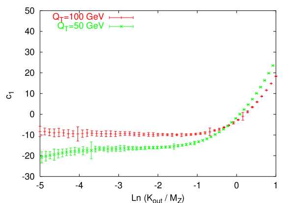
Figure 1: The first order coefficient function $c_{1}$ as a function of $K_{\mbox{\scriptsize out}}$ for the two values $Q_{m}=50,100\mathop{\rm Ge\!V}$ and $K=M$.

Given $c_{1}$ in (59) we now reconstruct the matched result. For instance, using the so called “log-R matching prescription”, to first order we have

$$\left[\,C_{\delta}(\alpha_{\mbox{\scriptsize s}})\,\right]^{\mbox{\scriptsize mat}}_{1}\>=\>e^{\frac{\alpha_{\mbox{\scriptsize s}}}{2\pi}c_{1}}\>.$$ (60)

It is straightforward to check that the distribution $\Sigma^{\mbox{\scriptsize PT}}$ obtained by using this coefficient function reproduces the exact result in (57) and accounts for all terms of the form $\alpha_{\mbox{\scriptsize s}}^{n}L^{2n-2}$ in the resummed expression (54). In order to obtain also the $\alpha_{\mbox{\scriptsize s}}^{n}L^{2n-3}$ terms one should perform a second order matching, which requires the fixed order exact result to order $\alpha_{\mbox{\scriptsize s}}^{2}$, not yet available.

Actually this expression for the distribution $\Sigma$ is not yet normalized to one at the maximum value $K_{\mbox{\scriptsize out}}^{M}$ of $K_{\mbox{\scriptsize out}}$. Indeed we used a normalization point at $K_{\mbox{\scriptsize out}}=K$, see (52). The standard way to achieve the correct normalization is to substitute

$$\begin{split}\frac{K}{K_{\mbox{\scriptsize out}}}\>\to\>\frac{K}{{\tilde{K}}_{\mbox{\scriptsize out}}}\equiv\frac{K}{K_{\mbox{\scriptsize out}}}-\frac{K}{K_{\mbox{\scriptsize out}}^{M}}+1\>,\qquad L\>\to\>\tilde{L}\equiv\ln\frac{M}{{\tilde{K}}_{\mbox{\scriptsize out}}}\>,\end{split}$$ (61)

in all previous expressions (except in $\Sigma_{1}^{\mbox{\scriptsize exact}}(Q_{m},K_{\mbox{\scriptsize out}})$ in (59) which is already correctly normalized). The variable $K_{\mbox{\scriptsize out}}$ goes to the correct kinematical boundary ($K_{\mbox{\scriptsize out}}\to K_{\mbox{\scriptsize out}}^{M}$) for ${\tilde{K}}_{\mbox{\scriptsize out}}\to K$ and tends to ${\tilde{K}}_{\mbox{\scriptsize out}}$ for small values.

6.3 Including the NP correction

We now discuss the full distribution including the leading NP corrections coming from the radiation factor. Recall that power corrections from ${\cal{P}}$ are subleading. The analysis is similar to the one in [2]. The NP radiator $\delta R_{\delta}$ is proportional to the Mellin variable $\nu$, see (47), and so it produces a shift of $K_{\mbox{\scriptsize out}}$

$$K_{\mbox{\scriptsize out}}\to K_{\mbox{\scriptsize out}}^{\prime}\equiv K_{\mbox{\scriptsize out}}-\delta K_{\mbox{\scriptsize out}}\,\qquad\delta K_{\mbox{\scriptsize out}}=\lambda^{\mbox{\scriptsize NP}}\,\Delta_{\delta}(K_{\mbox{\scriptsize out}})\>.$$ (62)

The final expression, including NP corrections, is then obtained from the PT result of previous subsections in which we replace $K_{\mbox{\scriptsize out}}$ with $K_{\mbox{\scriptsize out}}^{\prime}$.

Here $\lambda^{\mbox{\scriptsize NP}}$ is expressed in terms of the NP parameter $\alpha_{0}(\mu_{I})$, see (98). To evaluate $\Delta_{\delta}$ we observe that (47) contains a $\ln|q_{3x}|$ term. The $q_{3x}$ distribution is given by the radiation factor (42) which leads to $|q_{3x}|\sim K_{\mbox{\scriptsize out}}$, so that a $\ln|q_{3x}|$ term produces a $\ln K_{\mbox{\scriptsize out}}$ contribution. We find (see Appendix E.2)

$$\begin{split}\Delta_{\delta}(K_{\mbox{\scriptsize out}})&=C^{(\delta)}_{1}(\eta_{0}-\eta_{3})+C^{(\delta)}_{2}(\eta_{0}+\eta_{3})+C^{(\delta)}_{3}\,\ln\frac{Q^{\mbox{\scriptsize NP}}}{K_{\mbox{\scriptsize out}}}\>,\\ \ln Q^{\mbox{\scriptsize NP}}&=\ln\zeta Q_{t}+\gamma_{E}+\psi\left(1+R^{\prime}\right)+\mbox{\small$\frac{1}{2}$}\psi\left(1+\frac{R^{\prime}}{2}\right)-\mbox{\small$\frac{1}{2}$}\psi\left(\frac{1+R^{\prime}}{2}\right),\end{split}$$ (63)

with $R^{\prime}$ given in (51). Notice that, expanding in powers of $R^{\prime}$, the $p_{3}$ contribution is

$$\ln\frac{Q^{\mbox{\scriptsize NP}}}{K_{\mbox{\scriptsize out}}}=\ln\frac{2\zeta Q_{t}}{K_{\mbox{\scriptsize out}}}+{\cal{O}}\left(R^{\prime}\right)\>.$$ (64)

The factor $2$ here is simply due to the fact that $p_{3}$ acquires a recoil which is equal to $K_{\mbox{\scriptsize out}}/2$ for small $R^{\prime}$.

The effect of the substitution in (62) is a deformation of the PT distribution. First of all the quantity (63) depends logarithmically on $K_{\mbox{\scriptsize out}}$ (both explicitly and through the SL function $R^{\prime}$). This implies that the PT curve is shifted by an amount which decreases with increasing $K_{\mbox{\scriptsize out}}$. Moreover, $\Delta_{\delta}(K_{\mbox{\scriptsize out}})$ depends also on the rapidity $y$ distributed according to the incoming parton distributions ${\cal{P}}_{\delta}(K_{\mbox{\scriptsize out}})$.

Here the situation is different from the case of broadening [8] or $T_{m}$ [2] in $e^{+}e^{-}$ annihilation in which one obtains very singular contributions to the shift of order $1/\sqrt{\alpha_{\mbox{\scriptsize s}}}$. The difference is due to the different kinematical situations. In the two $e^{+}e^{-}$ cases one has to consider contributions in which some hard partons are forced to stay in the event plane. Then the PT distribution is given by a Sudakov form factor and then the $1/\sqrt{\alpha_{\mbox{\scriptsize s}}}$ contribution comes from the integration of the logarithmic term in the hard parton recoil. For the present observable instead, $p_{3}$ is not kinematically forced into the event plane and then its PT radiation factor reproduces a logarithmic contribution.

6.4 Numerical analysis

We report here some numerical results. We consider $p\bar{p}$ collisions at Tevatron energy ($\sqrt{s}=1.8$TeV) for some typical values of $Q_{m}$. Data on the $K_{\mbox{\scriptsize out}}$ distribution are not yet available. The results depend on the two parameters $\alpha_{\overline{\mbox{\scriptsize MS}}}(M_{Z})$ and $\alpha_{0}(\mu_{I})$ (with $\mu_{I}=2\mathop{\rm Ge\!V}$) which values we fix in the range determined by the $2$-jet shape analysis [20].

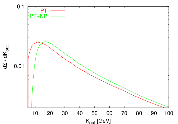
Figure 2: The differential distribution in (65) as function of $K_{\mbox{\scriptsize out}}$. We plot both the PT resummed and matched result and the full distribution including NP correction for $Q_{m}=50\mathop{\rm Ge\!V}$. Here we have taken $\alpha_{\overline{\mbox{\scriptsize MS}}}(M_{Z})=0.120$ and the NP parameter $\alpha_{0}(2\mathop{\rm Ge\!V})=0.52$. The contribution due to the beam remnant interaction is not included, it is given by a rigid shift in $K_{\mbox{\scriptsize out}}$ by $K_{\mbox{\scriptsize out}}^{\mbox{\scriptsize remnant}}$ of the order of few GeV, see (10).

In figs. 2, 3 we plot the differential distributions

$$\frac{d\Sigma(Q_{m},K_{\mbox{\scriptsize out}})}{dK_{\mbox{\scriptsize out}}}\>,$$ (65)

for two values of $Q_{m}$. The PT curve represents (54) with the coefficient function given by (60). We have performed the substitution (61) in order to take into account the correct normalization at the kinematical boundary. The rapidity cut is set at $\eta_{0}=2$. For simplicity we have taken the hard scale $K$ at $M$. We used the incoming parton distribution of [21].

The PT$+$NP curve is given by the above PT expression in which we make the substitution $K_{\mbox{\scriptsize out}}$ into $K_{\mbox{\scriptsize out}}^{\prime}$ according to (62). The leading NP correction is determined by the single parameter $\alpha_{0}(\mu_{I})$.

As discussed before, the effect of the NP substitution (62) is a deformation of the PT distribution. In particular the PT peak is shifted by about $10$ GeV. This effect, due to the QCD running coupling in the infrared region, has to be contrasted with the contribution from the beam remnant interaction which corresponds to a “rigid shift” of the hard QCD result by an amount $K_{\mbox{\scriptsize out}}^{\mbox{\scriptsize remnant}}$ of order of few GeV, see [14, 16, 17], proportional to $\eta_{0}$ but independent of the hard scales (see (10)).

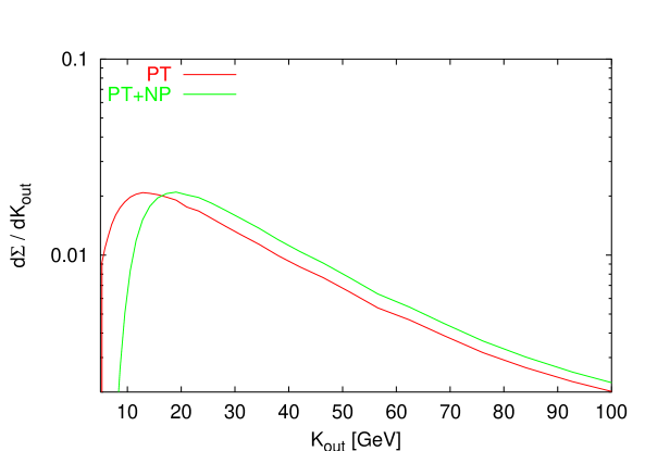
Figure 3: Same as fig. 2 for $Q_{m}=100\mathop{\rm Ge\!V}$.

7 Discussion and conclusion

The aim of the present study is the understanding of the structure of radiation in hard hh-collisions within the standard QCD treatment. We have introduced the jet-shape observable $K_{\mbox{\scriptsize out}}$ which is the extension to hh-collisions of $T_{m}$ in $e^{+}e^{-}$ annihilation. The hard QCD analysis includes next-to-leading order PT resummation, matching with exact first order result, and leading NP power corrections (arising from the fact that the running coupling argument runs into the infrared region). To avoid measurements inside the beam direction we have included a rapidity cut $\eta_{0}$ (see (4)). For values of $K_{\mbox{\scriptsize out}}$ much smaller than $K_{\mbox{\scriptsize out}}^{c}$ (of the order of $10$ GeV for $\eta_{0}=2$) there are powers of $\ln K_{\mbox{\scriptsize out}}/K_{\mbox{\scriptsize out}}^{c}$. In our calculation we consider the region $K_{\mbox{\scriptsize out}}>K_{\mbox{\scriptsize out}}^{c}$ so that we do not need to resum them. As a result the PT contribution does not depend on $\eta_{0}$. The dependence on $\eta_{0}$ enters only in the NP correction which corresponds to the substitution (62) in the argument of the PT distribution.

We discuss now some of the features of our hard QCD result.

In the present calculation we have various hard scales. It is then important to identify the specific hard scales in the various factorized pieces of the result (54). We find that $K_{\mbox{\scriptsize out}}$ is the hard scale for the incoming partons distribution ${\cal{P}}_{\delta}$ while it is the lower bound for frequencies contributing to the radiation factor ${\cal{A}}_{\delta}$. This result is based on the different rôle of real/virtual cancellations in the collinear singular quantity ${\cal{P}}_{\delta}$ and in the CIS radiation factor ${\cal{A}}_{\delta}$. Technically, in the present treatment, the factorization (${\cal{P}}_{\delta}\cdot{\cal{A}}_{\delta}$) results from (31) while real/virtual cancellation from (36). The hard scales for ${\cal{A}}_{\delta}$ are given by $Q_{a}^{(\delta)}\sim\sqrt{\hat{s}}$, the scales of the elementary hard process. They are identified at SL level and depend on the geometry of the event ($\hat{s}$- and $Q_{t}$-dependence) and on the configuration $\delta=q\bar{q},qg,gq$ for the two incoming partons. Therefore, the shape in $K_{\mbox{\scriptsize out}}$ of the distribution (at fixed $s$ and $Q_{m}$) depends on the weight of the various configurations. By changing $s$ and $Q_{m}$ one may be able to study the three configurations separately.

Leading power corrections come from the radiation factor (power corrections in the incoming parton distributions are subleading [5] and were not considered). They enter as a shift in the PT distribution given by (62). This is a feature common to all observables linear in the transverse momentum. The strength of the power correction is given by the NP parameter $\lambda^{\mbox{\scriptsize NP}}$ (expressed in terms of $\alpha_{0}(\mu_{I})$, see (98)), the same as introduced for the $e^{+}e^{-}$ jet-shape observables. The structure of the shift is characteristic of the fact that the observable $K_{\mbox{\scriptsize out}}$ is uniform in rapidity, see the discussions after (49) and (64). The NP shift is larger then the corresponding NP shift for 2-jet observables since it takes contributions from three hard partons, one of which is a gluon. This was also the case for the near to planar $3$-jet observables in $e^{+}e^{-}$ [2, 3]. We then expect that higher order NP effects may come into play near the peak of the distribution. This calls for a deeper analysis that would address higher power corrections, for example, along the lines of Korchemsky-Sterman approach which was recently developed for some 2-jet observables in [22]. The comparison with experimental data (not yet available) would shed light on this important point.

Numerical programs for exact results on the matrix elements for the process (1) are available [19] to order $\alpha_{\mbox{\scriptsize s}}^{2}$. Thus we have been able to compute only the first term of the coefficient function $C_{\delta}(\alpha_{\mbox{\scriptsize s}})$.

In $e^{+}e^{-}$ annihilation the hard QCD analysis described above has been shown to be sufficient to make quantitative predictions and study the universality of NP effects. In hh-collisions however we also need to take into account contributions coming from the soft underlying event due to beam remnant interaction. With the hypothesis that such contributions are factorized and independent of the hard scales (see [14, 16, 17] and Appendix G), they give rise to a “rigid shift” in $K_{\mbox{\scriptsize out}}$ by the amount $K_{\mbox{\scriptsize out}}^{\mbox{\scriptsize remnant}}$ (see (10)). This quantity, of the order of few GeV, is proportional to $\eta_{0}$ and the minimum bias parameters ${\cal{N}}$ and $\left\langle k_{t}\right\rangle^{\mbox{\scriptsize remnant}}$. The last two parameters should be the same in all hard hh-processes and could be determined and checked in the study of various observables.

This completes the analysis of our jet-shape observable in hard hh-collisions. The results depend on the two parameters $\alpha_{\mbox{\scriptsize s}}(M_{Z})$ and $\alpha_{0}(\mu_{I}=2\mathop{\rm Ge\!V})$. The important question is then whether the present QCD standard treatment is sufficient to reproduce the data in hard hh-collisions. In particular, our results should provide solid ground to study whether there is any need for non-hard QCD contributions.

Appendix A Elementary cross sections

We present the three elementary cross sections relating to the configurations $q\bar{q}$, $qg$ and $gq$ in terms of the kinematical variables $\hat{s}$ and $\theta$ introduced in equation (13).

The parton-level cross section $\hat{\sigma}_{\delta}^{f}$ for quark flavour $f$ and configuration $\delta$ is

$$\hat{\sigma}_{\delta}^{f}=\frac{1}{2\hat{s}}\int d\mbox{Lips}[P_{1}P_{2}\to QP_{3}]\cdot|M_{\delta}^{f}|^{2}\>,$$ (66)

where the Lorentz-invariant integration measure, after eliminating a trivial azimuthal angle, becomes simply

$$\int d\mbox{Lips}[P_{1}P_{2}\to QP_{3}]=\frac{\hat{s}-M^{2}}{16\pi\hat{s}}\int d\cos\theta\>.$$ (67)

For the matrix elements $M_{\delta}^{f}$ only the simple $2\to 2$ tree-level diagrams are required. After averaging over colours and spins we obtain

$$\begin{split}&|M_{q\bar{q}}^{f}|^{2}=\frac{32\pi^{2}\alpha_{\mbox{\scriptsize s}}\alpha_{f}C_{F}}{N_{c}}\frac{(P_{1}Q)^{2}+(P_{2}Q)^{2}}{(P_{1}P_{3})(P_{2}P_{3})}\\ &|M_{qg}^{f}|^{2}=\frac{32\pi^{2}\alpha_{\mbox{\scriptsize s}}\alpha_{f}T_{R}}{N_{c}}\frac{(P_{1}Q)^{2}+(P_{3}Q)^{2}}{(P_{1}P_{2})(P_{2}P_{3})}\\ &|M_{gq}^{f}|^{2}=\frac{32\pi^{2}\alpha_{\mbox{\scriptsize s}}\alpha_{f}T_{R}}{N_{c}}\frac{(P_{2}Q)^{2}+(P_{3}Q)^{2}}{(P_{1}P_{2})(P_{1}P_{3})}\>,\end{split}$$ (68)

where $\alpha_{f}$ is the electroweak coupling of the quark to the $Z_{0}$

$$4\pi\alpha_{f}=\left(\frac{g_{W}}{2\cos\theta_{W}}\right)^{2}\left(V_{f}^{2}+A_{f}^{2}\right)\>.$$ (69)

Using (13) to express these matrix elements in terms of $\hat{s}$ and $\theta$ quickly yields the differential cross sections

$$\begin{split}\frac{d\hat{\sigma}^{f}_{q\bar{q}}(\hat{s},\theta)}{d\cos\theta}&=\>\frac{2\pi\alpha_{\mbox{\scriptsize s}}\alpha_{f}C_{F}}{N_{c}}\cdot\frac{2(E^{2}+p^{2}\cos^{2}\theta)}{p\,\hat{s}^{3/2}\sin^{2}\theta}\>,\\ \frac{d\hat{\sigma}^{f}_{qg}(\hat{s},\theta)}{d\cos\theta}&=\>\frac{2\pi\alpha_{\mbox{\scriptsize s}}\alpha_{f}T_{R}}{N_{c}}\cdot\frac{(E-p\cos\theta)^{2}+4p^{2}}{\hat{s}^{2}(1-\cos\theta)}\,\\ \frac{d\hat{\sigma}^{f}_{gq}(\hat{s},\theta)}{d\cos\theta}&=\>\frac{2\pi\alpha_{\mbox{\scriptsize s}}\alpha_{f}T_{R}}{N_{c}}\cdot\frac{(E+p\cos\theta)^{2}+4p^{2}}{\hat{s}^{2}(1+\cos\theta)}\,\end{split}$$ (70)

We however are interested in $d\hat{\sigma}_{\delta}^{f}/dQ_{t}$, which is given by

$$\frac{d\hat{\sigma}_{\delta}^{f}(\hat{s},Q_{t})}{dQ_{t}}=\int_{-1}^{1}d\cos\theta\,\delta(Q_{t}-p\sin\theta)\,\frac{d\hat{\sigma}_{\delta}^{f}(\hat{s},\theta)}{d\cos\theta}\>.$$ (71)

On integrating over $\theta$ there are contributions from $\cos\theta=\pm\sqrt{1-Q_{t}^{2}/p^{2}}$. Thus

$$\frac{d\hat{\sigma}_{\delta}^{f}(\hat{s},Q_{t})}{dQ_{t}}=\left.\frac{\tan\theta}{p}\frac{d\hat{\sigma}_{\delta}^{f}}{d\cos\theta}\right|_{\cos\theta>0}-\left.\frac{\tan\theta}{p}\frac{d\hat{\sigma}_{\delta}^{f}}{d\cos\theta}\right|_{\cos\theta<0}\>.$$ (72)

Now we make use of the fact that, for proton-proton and proton-antiproton collisions, these two terms contribute equally to (14). (This would not of course be true for collisions of two arbitrary hadrons.) Therefore we may take $\cos\theta>0$ and write

$$\frac{d\hat{\sigma}_{\delta}^{f}(\hat{s},Q_{t})}{dQ_{t}}=2\frac{\tan\theta}{p}\frac{d\hat{\sigma}_{\delta}^{f}(\hat{s},\theta)}{d\cos\theta}\>,\quad\quad\sin\theta=Q_{t}/p\>,\quad\cos\theta=\sqrt{1-Q_{t}^{2}/p^{2}}\>.$$ (73)

The relation $\sin\theta=Q_{t}/p$ gives a lower bound on the total centre of mass energy $\sqrt{\hat{s}}$:

$$\sqrt{\hat{s}}>\sqrt{\hat{s}_{0}}=Q_{t}+\sqrt{M^{2}+Q_{t}^{2}}\>.$$ (74)

Finally, a consideration of the kinematics shows that, for fixed partonic energy $\sqrt{\hat{s}}$ the observable is bounded by

$$K_{\mbox{\scriptsize out}}^{2}<\hat{s}+M^{2}-2\sqrt{\hat{s}(Q_{t}^{2}+M^{2})}\>,$$ (75)

and since $Q_{t}$ can be as low as $Q_{m}$ and $\hat{s}$ can (with small probability) be as large as $s$, we have the absolute upper bound

$$K_{M}^{2}=s+M^{2}-2\sqrt{s(Q_{m}^{2}+M^{2})}\>.$$ (76)

Appendix B Incoming parton evolution at the hard scale

We denote by $s_{ab}$ the contribution to $\Gamma_{\delta}$ from a given $ab$-dipole distribution $w_{ab}$, see (29), and consider first the $12$-dipole contribution

$$s_{12}=\sum_{a=1}^{2}\int_{{\cal{C}}_{a}}\frac{d^{3}k}{\pi\omega}w_{12}(k)(1-z^{N_{a}-1})\,u(k_{x})=\sum_{a=1}^{2}S_{1}(N_{a})\int\frac{d^{2}k_{t}}{\pi k_{t}^{2}}\frac{\alpha_{\mbox{\scriptsize s}}(k_{t})}{\pi}\,e^{-\nu(|k_{x}|-i\beta k_{x})}\>,$$ (77)

with

$$S_{1}(N)=\int_{0}^{1}dz\;\frac{1-z^{N-1}}{1-z}=\sum_{n=1}^{N-1}\frac{1}{n}\>,$$ (78)

proportional to the soft piece of the anomalous dimension. Here both collinear regions ${\cal{C}}_{1},{\cal{C}}_{2}$ contribute.

The contribution from the other two radiators $s_{13},s_{23}$ is similar. They take a contribution from a single collinear region (the $a3$-dipole from the region ${\cal{C}}_{a}$ collinear to $p_{a}$), so that

$$s_{a3}=S_{1}(N_{a})\int\frac{d^{2}k_{t}}{\pi k_{t}^{2}}\frac{\alpha_{\mbox{\scriptsize s}}(k_{t})}{\pi}\,e^{-\nu(|k_{x}|-i\beta k_{x})}\>,\qquad a=1,2\>.$$ (79)

Since the $s_{ab}$ are singular for $k_{x}\to 0$, one needs to introduce a cutoff $\mu$ on the $k_{t}$ integral. We also use the fact that, to our required accuracy, the $k_{x}$-source can be replaced by an effective cutoff (see (36)). We are therefore required to integrate over a region in $k_{x},k_{y}$-space given by $\Theta(\rho^{-1}-|k_{x}|)\Theta(k_{t}-\mu)$, where we choose $\mu$ to be less than $\rho^{-1}$. So, to SL accuracy, we write (for instance for the $a3$-dipole)

$$s_{a3}=S_{1}(N_{a})\int_{\mu}^{1/\rho}\frac{dk_{t}}{k_{t}}\frac{2\alpha_{\mbox{\scriptsize s}}(k_{t})}{\pi}\>,$$ (80)

where the remainder is beyond our required SL accuracy.

As anticipated, since here one has $|k_{x}|<\rho^{-1}\ll Q_{t}$, the precise definition of the collinear regions ${\cal{C}}_{1},{\cal{C}}_{2}$ is not important.

Appendix C The PT radiator

The PT radiator is given, to SL accuracy, in terms of $ab$-dipole radiators

$$r_{ab}(\nu,\beta)=\int\frac{d^{3}k}{\pi\omega}w_{ab}(k)\,\left[1-e^{-\nu(|k_{x}|-i\beta k_{x})}\right],\qquad w_{ab}(k)=\frac{\alpha_{\mbox{\scriptsize s}}(k^{2}_{ab,t})}{\pi k^{2}_{ab,t}}\>,$$ (81)

where $k_{ab,\,t}$ is the invariant transverse momentum of $k$ with respect to the $P_{a},P_{b}$ hard partons in (13). For the configuration $\delta=q\bar{q}$, for instance, we have

$$R^{\mbox{\scriptsize PT}}_{q\bar{q}}(\nu,\beta)=\frac{N_{c}}{2}\left(r_{13}(\nu,\beta)+r_{23}(\nu,\beta)-\frac{1}{N_{c}^{2}}\,r_{12}(\nu,\beta)\right).$$ (82)

To evaluate the $ab$-dipole radiator $r_{ab}(\nu,\beta)$ we work in the centre of mass system of the $ab$-dipole. We neglect at this stage the rapidity cut (4): we will show at the end of this appendix that the difference is beyond our accuracy. Denoting by $P^{*}_{a},P^{*}_{b}$ and $k^{*}$ the momenta in this system, we introduce the Sudakov decomposition

$$P_{a}^{*}=\frac{Q_{ab}}{2}(1,0,0,1)\>,\quad P_{b}^{*}=\frac{Q_{ab}}{2}(1,0,0,-1)\>,\qquad k^{*}=\alpha P_{a}^{*}+\beta P_{b}^{*}+\kappa\>,$$ (83)

where $Q_{ab}^{2}=2(P_{a}P_{b})$ so that (13) gives

$$Q^{2}_{12}=\hat{s}\>,\quad Q^{2}_{13}=p\sqrt{\hat{s}}\,(1+\cos\theta)\>,\quad Q^{2}_{23}=p\sqrt{\hat{s}}\,(1-\cos\theta)\>,$$ (84)

and $\theta$ is given in equation (73). Here the two-dimensional vector $\vec{\kappa}$ is the transverse momentum orthogonal to the $ab$-dipole momenta ($\kappa^{2}=k^{2}_{ab,t}$). We have then

$$w_{ab}(k)=\frac{\alpha_{\mbox{\scriptsize s}}(\kappa^{2})}{\pi\kappa^{2}}\>,\qquad\frac{d^{3}k}{\pi\omega}=\frac{d^{2}\kappa}{\pi}\frac{d\alpha}{\alpha}\>,\quad\alpha>\frac{\kappa^{2}}{Q^{2}_{ab}}\>.$$ (85)

Since, neglecting the recoil $q_{3}$, the outgoing momentum $P_{3}$ is in the $yz$-plane, the Lorentz transformation is in the $yz$-plane and our observable $k_{x}$ remains unchanged. The $ab$-radiator has then the form

$$r_{ab}(\nu,\beta)=2\int_{0}^{Q^{2}_{ab}}\frac{d^{2}\kappa}{\pi\kappa^{2}}\frac{\alpha_{\mbox{\scriptsize s}}(\kappa)}{\pi}\int_{\kappa/Q_{ab}}^{1}\frac{d\alpha}{\alpha}\left[1-e^{-\nu(|k_{x}|-i\beta k_{x})}\right],\quad\kappa_{x}=k_{x}\>,$$ (86)

where the factor $2$ comes because we have integrated only over the “right hemisphere” $\alpha>\kappa/Q_{ab}$. Integrating over $\alpha$ and $\kappa_{y}$ we have

$$r_{ab}(\nu,\beta)=2\int_{-Q_{ab}}^{Q_{ab}}\frac{dk_{x}}{|k_{x}|}\left[1-e^{-\nu(|k_{x}|-i\beta k_{x})}\right]\cdot\frac{\alpha_{\mbox{\scriptsize s}}(2|k_{x}|)}{\pi}\ln\frac{Q_{ab}}{2|k_{x}|}\>.$$ (87)

To show this we introduced $\kappa_{y}=t\cdot|k_{x}|$ and used

$$\int_{-\infty}^{\infty}\frac{dt}{\pi(1+t^{2})}\alpha_{\mbox{\scriptsize s}}\left(|k_{x}|\sqrt{1+t^{2}}\right)\ln\frac{Q_{ab}}{|k_{x}|\sqrt{1+t^{2}}}\simeq\alpha_{\mbox{\scriptsize s}}(2|k_{x}|)\ln\frac{Q_{ab}}{2|k_{x}|}\>.$$ (88)

We extended the $t$-integration to infinity since it is convergent, then we integrated over $t$ by expanding $\alpha_{\mbox{\scriptsize s}}$ to second order. Corrections are beyond SL accuracy. Finally, using (36), we obtain

$$r_{ab}(\nu,\beta)=4\int_{\rho^{-1}}^{Q_{ab}}\frac{dk_{x}}{k_{x}}\frac{\alpha_{\mbox{\scriptsize s}}(2k_{x})}{\pi}\>\ln\frac{Q_{ab}}{2k_{x}}\>.$$ (89)

Assembling the various dipole contributions and including hard collinear splittings then yields, to SL accuracy, (44) and (45).

We now show that the rapidity cut (4) is negligible for the PT radiator. The difference between the radiator with the cut imposed and that without is given by the dipole contributions

$$\Delta r_{ab}(\nu,\beta)=-\int_{|\eta_{k}|>\eta_{0}}\frac{d^{3}k}{\pi\omega}\>w_{ab}(k)\>e^{i\nu\beta k_{x}}\left(1-e^{-\nu|k_{x}|}\right)\>.$$ (90)

In order to implement the rapidity cut, we express $\eta_{k}$ the soft gluon rapidity in the frame (3) in the invariant form:

$$\eta_{k}=\frac{1}{2}\ln\frac{(h_{2}k)}{(h_{1}k)}=y+\frac{1}{2}\ln\frac{(P_{2}k)}{(P_{1}k)}\>,$$ (91)

where $h_{1},h_{2}$ are the incoming hadron momenta in (3) and $P_{1},P_{2},y$ are the hard incoming parton momenta and rapidity in (13).

For the $12$ dipole we have $\eta_{k}=y+\ln(\alpha Q_{12}/\kappa)$, and thus we obtain from the “right” hemisphere

$$\Delta r_{12}(\nu,\beta)=-\int_{0}^{Q_{12}^{\prime}}\frac{d^{2}\kappa}{\pi\kappa^{2}}\frac{\alpha_{\mbox{\scriptsize s}}(\kappa)}{\pi}\int_{\kappa/Q_{12}^{\prime}}^{1}\frac{d\alpha}{\alpha}\>e^{i\nu\beta k_{x}}\left(1-e^{-\nu|k_{x}|}\right)\>,\quad Q_{12}^{\prime}=Q_{12}e^{y-\eta_{0}}\>.$$ (92)

Here the scale for the correction is $Q_{12}^{\prime}\sim K_{\mbox{\scriptsize out}}^{c}\leq{\cal{O}}\left(\nu^{-1}\right)$ and so the contribution is of order $\alpha_{\mbox{\scriptsize s}}(K_{\mbox{\scriptsize out}})$ without a logarithmic enhancement. The same is found for the “left” hemisphere contribution.

For the $13$ dipole we obtain a similar result for the cut around the $P_{1}$ direction, (using (105) to evaluate $\eta_{k}$), while the cut around the $P_{2}$ direction gives a tiny correction proportional to the size of the hole: the converse holds for the $23$ dipole.

Appendix D NP corrections to the radiator

We consider the NP correction $\delta r_{ab}$ to the $ab$-dipole radiator. In this case, as we shall see, we need to retain both the recoil $q_{3x}$ and the rapidity cut $\eta_{0}$ (recall that in the PT component they both gave subleading effects and were neglected). We write the integral in the $ab$-dipole centre of mass variables $\alpha,\beta$ and $\vec{\kappa}$ introduced in (83) and, to obtain the NP correction $\delta r_{ab}$, we perform the following standard operations:

• the running coupling, reconstructed by two loop emission, is represented by the dispersive form [5]. Then, the $ab$-dipole radiation $w_{ab}(k)$ is written in the $ab$-centre of mass system (see (85)) in the form

  $$w_{ab}(k)=\frac{\alpha_{\mbox{\scriptsize s}}(\kappa)}{\pi\kappa^{2}}=\int_{0}^{\infty}\frac{dm^{2}\,\alpha_{\mbox{\scriptsize eff}}(m)}{\pi(\kappa^{2}+m^{2})^{2}}\>;$$ (93)

• to take into account the emission of soft partons at two loop order [6], we need to extend the source $u(k_{x})$ to include the mass $m$ of the soft system. We assume $k_{x}=\kappa\cos\phi\to\sqrt{\kappa^{2}+m^{2}}\cos\phi$, with $\phi$ the azimuthal angle of $\vec{\kappa}$. Similarly we introduce the mass in the kinematical relations such as $\alpha\beta=(\kappa^{2}+m^{2})/Q_{ab}^{2}$ for the $ab$-dipole variables;

• we take the NP part $\delta\alpha_{\mbox{\scriptsize eff}}(m)$ of the effective coupling. Since it has support only for small $m$, we take the leading part of the integrand for small $\kappa$, and $m$. In particular we linearize the source $U(k)$

  $$\left[1-U(k)\right]\>\to\>\nu\sqrt{\kappa^{2}+m^{2}}\>|\cos\phi|\>\Theta(\eta_{0}-|\eta_{k}|)\>.$$ (94)

  Recall that $\eta_{k}$ is the rapidity of $k$ in the laboratory system (3). Here we have neglected terms proportional to $\beta$ since they vanish, by symmetry, upon the $\beta$ integration;

• the recoil component $q_{3x}$ of the outgoing parton does provide an effective cut in the soft gluon rapidity along the outgoing parton [2, 8]. This is due to a real-virtual cancellation which takes place when the angle of the outgoing parton $p_{3}$ with the event plane exceeds the corresponding angle of the soft gluon. The detailed analysis of real and virtual pieces entails that the contribution from the observable $\sqrt{\kappa^{2}+m^{2}}\>|\cos\phi|$ in the linear expansion of the source (see (94)) has to be replaced by

  $$\sqrt{\kappa^{2}+m^{2}}\>|\cos\phi|\to\left|\sqrt{\kappa^{2}+m^{2}}\,\cos\phi+\alpha q_{3x}\right|-\alpha|q_{3x}|\>,$$ (95)

  with $\alpha$ the Sudakov variable in the $a3$-dipole centre of mass;

• to take fully into account effects of non-inclusiveness of jet observables at two-loop order, we multiply the radiator by the Milan factor [6, 7]

  $${\cal{M}}=\frac{3}{64}\frac{(128\pi+128\pi\ln 2-35\pi^{2})C_{A}-5\pi^{2}n_{f}}{11C_{A}-2n_{f}}\>,$$ (96)

  using $n_{f}=3$;

• the NP correction is finally expressed in terms of the parameter

  $$\lambda^{\mbox{\scriptsize NP}}=2{\cal{M}}\,c_{K_{\mbox{\scriptsize out}}}\int dm\frac{\delta\alpha_{\mbox{\scriptsize eff}}(m)}{\pi}\>,\quad c_{K_{\mbox{\scriptsize out}}}=\frac{2}{\pi}\>.$$ (97)

  After merging PT and NP contributions to the observable in a renormalon free manner, one has that the distribution is independent of $\mu_{I}$ and one obtains

  $$\lambda^{\mbox{\scriptsize NP}}\!\equiv c_{K_{\mbox{\scriptsize out}}}\,{\cal{M}}\frac{4}{\pi^{2}}\mu_{I}\left\{\alpha_{0}(\mu_{I})-\bar{\alpha}_{s}-\beta_{0}\frac{\bar{\alpha}_{s}^{2}}{2\pi}\left(\ln\frac{Q}{\mu_{I}}+\frac{K}{\beta_{0}}+1\right)\right\},$$ (98)

  where

  $$\bar{\alpha}_{s}\equiv\alpha_{\overline{\mbox{\scriptsize MS}}}(Q)\>,\quad K\equiv C_{A}\left(\frac{67}{18}-\frac{\pi^{2}}{6}\right)-\frac{5}{9}n_{f}\>,\quad\beta_{0}=\frac{11N_{c}}{3}-\frac{2n_{f}}{3}\>.$$ (99)

  The $K$ factor accounts for the mismatch between the $\overline{\mbox{\scriptsize MS}}$ and the physical scheme [18] and $\alpha_{0}(\mu_{I})$ is given in (48). Here $Q$ is the renormalisation scale used in the next-to-leading order PT calculation.

  The numerical coefficient $c_{K_{\mbox{\scriptsize out}}}$ depends on our observable $K_{\mbox{\scriptsize out}}$. For instance, the shift for the $\tau=1\!-\!T$ distribution is

  $$\frac{d\sigma}{d\tau}(\tau)=\frac{d\sigma^{\mbox{\scriptsize PT}}}{d\tau}(\tau\!-\!\Delta_{\tau})\>,\qquad\Delta_{\tau}=C_{F}\,\frac{c_{\tau}\,\lambda^{\mbox{\scriptsize NP}}}{c_{K_{\mbox{\scriptsize out}}}}\>,\quad c_{\tau}=2\>,$$ (100)

  where $C_{F}$ enters due to the fact the two-jet system is made of a quark-antiquark pair.

We recall that these prescriptions correspond to taking into account NP corrections at two-loop order in the reconstruction of the (dispersive) running coupling and in the non-inclusive nature of the observable. We implement the rapidity cut by expressing $\eta_{k}$ the soft gluon rapidity in the invariant form (91).

D.1 Dipole $12$

This procedure gives, for the $12$-dipole contribution,

$$\begin{split}\delta r_{12}&=\frac{\nu{\cal{M}}}{\pi}\!\int\!dm^{2}\delta\alpha_{\mbox{\scriptsize eff}}(m)\frac{-d}{dm^{2}}\!\int\frac{d\kappa^{2}}{\kappa^{2}+m^{2}}\int_{-\pi}^{\pi}\frac{d\phi}{2\pi}\sqrt{\kappa^{2}+m^{2}}|\cos\phi|\cdot 2\eta_{0}\\ &=\nu\,\lambda^{\mbox{\scriptsize NP}}\>2\eta_{0}\>.\end{split}$$ (101)

We used the $12$-dipole centre of mass variables $\alpha,\beta$ and $\vec{\kappa}$ introduced in (83). This result is found by using (91) and

$$\frac{P_{2}k}{P_{1}k}=\frac{\alpha}{\beta}=\frac{(\alpha Q_{12})^{2}}{\kappa^{2}+m^{2}}\>,$$ (102)

so that the $\alpha$ integration yields

$$\int_{0}^{1}\frac{d\alpha}{\alpha}\Theta\left(\eta_{0}-\left|\ln\frac{\alpha Q_{12}e^{y}}{\sqrt{\kappa^{2}+m^{2}}}\right|\right)\to 2\eta_{0}\>,\qquad\kappa,m\to 0\>.$$ (103)

The observable is uniform in rapidity and its integration gives $2\eta_{0}$. Corrections coming from the presence of the recoil $q_{3x}$ can be neglected in this case.

D.2 Dipoles $13$ and $23$

We consider now the NP corrections $\delta r_{a3}$ to the $a3$-dipole radiators and again we use the $a3$-dipole centre of mass variables $\alpha,\beta$ and $\vec{\kappa}$ introduced in (83). The situation is different from the previous $12$-case in two respects.

First of all we have that the $\eta_{0}$ cut in the soft gluon rapidity $\eta_{k}$ does not affect the region along the hard outgoing parton $p_{3}$. There one has to take into account that, as in the case of broadening [8] or thrust minor [2], the recoil component $q_{3x}$ of the outgoing parton provides an effective cut in the soft gluon rapidity. If the three momenta in this system are given by the Sudakov decomposition

$$P_{3}^{*}=\frac{Q_{a3}}{2}(1,0,0,1)\>,\quad P_{a}^{*}=\frac{Q_{a3}}{2}(1,0,0,-1)\>,\qquad k^{*}=\alpha P_{3}^{*}+\beta P_{a}^{*}+\kappa\>,$$ (104)

we are required to use the expression given in (95) as our linearized source.

The second complication for the $a3$ case is that the expression of $|\eta_{k}|$ in terms of the variables in (104) is rather complex, due to the fact that the Lorentz transformation to go from (13) to (104) involves both a $yz$-rotation and a boost along the $y$-axis. For our analysis, we need the expression for $\eta_{k}$ only for the soft gluon close to the incoming parton direction.

We consider first the case of $13$-dipole. For ${k}$ nearly parallel to ${P}_{1}$ we have $\beta\gg\alpha$ and this gives

$$\frac{P_{2}k}{P_{1}k}\simeq\left(\frac{Q_{12}}{Q_{13}}\right)^{2}\cdot\frac{\kappa^{2}+m^{2}}{(\alpha Q_{13})^{2}}\>,$$ (105)

The NP correction to the $13$-dipole radiator is then given by

$$\begin{split}\delta r_{13}&=\frac{\nu{\cal{M}}}{\pi}\!\int\!dm^{2}\delta\alpha_{\mbox{\scriptsize eff}}(m)\frac{-d}{dm^{2}}\!\int\frac{d\kappa^{2}}{\kappa^{2}+m^{2}}\cdot I_{13}\>,\\ I_{13}&=\int_{-\pi}^{\pi}\frac{d\phi}{2\pi}\int_{0}^{1}\frac{d\alpha}{\alpha}\left(\left|\sqrt{\kappa^{2}\!+\!m^{2}}\cos\phi\!+\!\alpha q_{3x}\right|\!-\!\alpha|q_{3x}|\right)\Theta\left(\eta_{0}+\ln\frac{\alpha Q^{2}_{13}\>e^{-y}}{Q_{12}\sqrt{\kappa^{2}+m^{2}}}\right).\end{split}$$ (106)

Again, in the region of $k^{*}$ emitted in the $P^{*}_{1}$ hemisphere ($\alpha<\sqrt{\kappa^{2}+m^{2}}/{Q_{13}}$) the rapidity cut $\eta_{0}$ gives the lower limit of the $\alpha$-integral. In the other region of $k^{*}$ emitted in the $P^{*}_{3}$ hemisphere ($\alpha>\sqrt{\kappa^{2}+m^{2}}/{Q_{13}}$) it is the recoil component $q_{3x}$ which provides the upper limit of $\alpha$. We have

$$\alpha_{m}<\alpha<\alpha_{M}\>,\qquad\alpha_{m}\equiv\frac{\sqrt{\kappa^{2}+m^{2}}\,Q_{12}\,e^{y-\eta_{0}}}{Q^{2}_{13}}\>,\quad\alpha_{M}\equiv{\frac{\sqrt{\kappa^{2}+m^{2}}}{|q_{3x}|}}\>,$$ (107)

giving

$$\begin{split}I_{13}&=\int_{-\pi}^{\pi}\frac{d\phi}{2\pi}\int_{\alpha_{m}}^{\alpha_{M}}\frac{d\alpha}{\alpha}\left(\left|\sqrt{\kappa^{2}\!+\!m^{2}}\cos\phi\!+\!\alpha q_{3x}\right|\!-\!\alpha|q_{3x}|\right)\\ &=\frac{2}{\pi}\sqrt{\kappa^{2}+m^{2}}\left(\eta_{0}-y+\ln\frac{Q_{13}}{Q_{12}}+\ln\frac{Q_{13}\zeta}{|q_{3x}|}\right),\qquad\zeta=2e^{-2}\>.\end{split}$$ (108)

Here $\zeta$ comes from the integration region of large rapidity of $k$ near $p_{3}$. In conclusion we have

$$\begin{split}\delta r_{13}=\nu\lambda^{\mbox{\scriptsize NP}}\left(\eta_{0}-y+\ln\frac{Q_{13}}{Q_{12}}+\ln\frac{Q_{13}\zeta}{|q_{3x}|}\right).\end{split}$$ (109)

A similar result is obtained from the last $23$-dipole radiator:

$$\delta r_{23}=\nu\lambda^{\mbox{\scriptsize NP}}\left(\eta_{0}+y+\ln\frac{Q_{23}}{Q_{12}}+\ln\frac{Q_{23}\zeta}{|q_{3x}|}\right)\>.$$ (110)

A compilation of these three contributions then gives the result (47).

Appendix E Distribution

E.1 Evaluation of ${\cal{A}}_{\delta}^{\mbox{\scriptsize PT}}$

Here we compute ${\cal{A}}^{\mbox{\scriptsize PT}}_{\delta}$ obtained from (41) by taking only the PT part of the radiator given in (44). Since $R^{\mbox{\scriptsize PT}}_{\delta}$ does not depend on the recoil, in (42) we can freely integrate over $q_{3x}$ to get

$${\cal{A}}^{\mbox{\scriptsize PT}}_{\delta}(\hat{s},Q_{t},K_{\mbox{\scriptsize out}})\>=\>\int\frac{d\nu\,e^{\nu K_{\mbox{\scriptsize out}}}}{2\pi i\nu}\>\int_{-\infty}^{\infty}\frac{d\beta\,e^{-R^{\mbox{\scriptsize PT}}_{\delta}\left(\bar{\nu}\sqrt{1+\beta^{2}}\right)}}{\pi(1+\beta^{2})}\>,\qquad\bar{\nu}=e^{\gamma_{E}}\nu\>.$$ (111)

We now perform the Mellin transform to SL accuracy. We make use of the operator identity

$$\int\frac{d\nu\,e^{\nu K_{\mbox{\scriptsize out}}}}{2\pi i\nu}\>G(\nu)=\frac{1}{\Gamma\left(1+\frac{\partial}{\partial\ln K_{\mbox{\scriptsize out}}}\right)}\>G(K_{\mbox{\scriptsize out}}^{-1})$$ (112)

for any logarithmically varying function $G$. (To prove this, multiply both sides by the $\Gamma$-function operator and use the definition $\Gamma(z)=\int_{0}^{\infty}dx\,x^{z-1}e^{-x}$.) Thus we obtain the quantity ${\cal{A}}_{\delta}^{\mbox{\scriptsize PT}}$ in the form

$${\cal{A}}_{\delta}^{\mbox{\scriptsize PT}}=\int_{-\infty}^{\infty}\frac{d\beta}{\pi(1+\beta^{2})}\>\frac{1}{\Gamma\left(1+\frac{\partial}{\partial\ln K_{\mbox{\scriptsize out}}}\right)}\>e^{-R^{\mbox{\scriptsize PT}}_{\delta}\left(\bar{K}_{\mbox{\scriptsize out}}^{-1}\sqrt{1+\beta^{2}}\right)}\>,\quad\bar{K}_{\mbox{\scriptsize out}}=e^{-\gamma_{E}}K_{\mbox{\scriptsize out}}\>.$$ (113)

We make a logarithmic expansion of the radiator, neglecting contributions from the second logarithmic derivative, which are beyond SL accuracy. So we obtain

$$\begin{split}&R_{\delta}^{\mbox{\scriptsize PT}}\left(\bar{K}_{\mbox{\scriptsize out}}^{-1}\sqrt{1+\beta^{2}}\right)=R_{\delta}^{\mbox{\scriptsize PT}}\left(K_{\mbox{\scriptsize out}}^{-1}\right)+\left(\gamma_{E}+\ln\sqrt{1+\beta^{2}}\right)R^{\prime}\>,\\ &R^{\prime}=-\frac{\partial}{\partial\ln K_{\mbox{\scriptsize out}}}R_{\delta}^{\mbox{\scriptsize PT}}\left(K_{\mbox{\scriptsize out}}^{-1}\right)\>.\end{split}$$ (114)

To SL accuracy, $R^{\prime}$ is given by (51).

Therefore we may write

$${\cal{A}}_{\delta}^{\mbox{\scriptsize PT}}=e^{-R^{\mbox{\scriptsize PT}}_{\delta}(K_{\mbox{\scriptsize out}}^{-1})}\frac{e^{-\gamma_{E}R^{\prime}}}{\Gamma(1+R^{\prime})}\>\int_{-\infty}^{\infty}\frac{d\beta}{\pi(1+\beta^{2})^{1+\frac{1}{2}R^{\prime}}}\>,$$ (115)

which leads immediately to the result (50).

E.2 Including the NP correction

The analysis is similar to the one in [2]. We report only the essential steps. Consider

$$\begin{split}\hat{\cal{A}}_{\delta}(\nu)&=\int_{-\infty}^{\infty}\frac{\nu d\beta dq_{3x}}{2\pi}e^{-\nu(|q_{3x}|-i\beta q_{3x})}e^{-R^{\mbox{\scriptsize PT}}_{\delta}\left(\bar{\nu}\sqrt{1+\beta^{2}}\right)}\\ &\qquad\times\left\{1-\nu\,\lambda^{\mbox{\scriptsize NP}}\,\left(C_{1}^{(\delta)}(\eta_{0}-\eta_{3})+C_{2}^{(\delta)}(\eta_{0}+\eta_{3})+C_{3}^{(\delta)}\ln\frac{\zeta Q_{t}}{|q_{3x}|}\right)\right\},\end{split}$$ (116)

where we have expanded $\exp(-\delta R_{\delta})$ to first order in order to obtain the leading correction. Performing the $q_{3x}$ integration we get

$$\hat{\cal{A}}_{\delta}(\nu)=\hat{\cal{A}}_{\delta}^{\mbox{\scriptsize PT}}(\nu)-\nu\,\lambda^{\mbox{\scriptsize NP}}\>f_{\delta}(\nu)\>,$$ (117)

where

$$f_{\delta}(\nu)\!=\!\!\int_{-\infty}^{\infty}\!\!\frac{d\beta\,e^{-R^{\mbox{\scriptsize PT}}_{\delta}\left(\bar{\nu}\sqrt{1+\beta^{2}}\right)}}{\pi(1+\beta^{2})}\left(C_{1}^{(\delta)}(\eta_{0}\!-\!\eta_{3})+C_{2}^{(\delta)}(\eta_{0}\!+\!\eta_{3})+C_{3}^{(\delta)}[\ln\zeta\bar{\nu}Q_{t}\!+\!\chi(\beta)]\right),$$ (118)

with $\chi(\beta)=\ln\sqrt{1+\beta^{2}}+\beta\tan^{-1}\beta$. This gives

$${\cal{A}}_{\delta}(K_{\mbox{\scriptsize out}})={\cal{A}}_{\delta}^{\mbox{\scriptsize PT}}(K_{\mbox{\scriptsize out}})+\delta{\cal{A}}_{\delta}(K_{\mbox{\scriptsize out}})\>,\quad\delta{\cal{A}}_{\delta}(K_{\mbox{\scriptsize out}})=-\lambda^{\mbox{\scriptsize NP}}\partial_{K_{\mbox{\scriptsize out}}}\int\frac{d\nu e^{\nu K_{\mbox{\scriptsize out}}}}{2\pi i\nu}\,f_{\delta}(\nu)\>.$$ (119)

From equation (112) and (119) we obtain

$$\begin{split}&\delta{\cal{A}}_{\delta}(K_{\mbox{\scriptsize out}})=\frac{-\lambda^{\mbox{\scriptsize NP}}}{K_{\mbox{\scriptsize out}}}\int_{-\infty}^{\infty}\frac{d\beta}{\pi(1+\beta^{2})}\frac{\frac{\partial}{\partial\ln K_{\mbox{\scriptsize out}}}}{\Gamma\left(1+\frac{\partial}{\partial\ln K_{\mbox{\scriptsize out}}}\right)}\\ &\times e^{-R^{\mbox{\scriptsize PT}}_{\delta}\left(\bar{K}_{\mbox{\scriptsize out}}^{-1}\sqrt{1+\beta^{2}}\right)}\left(C_{1}(\eta_{0}-\eta_{3})+C_{2}(\eta_{0}+\eta_{3})+C_{3}[\ln(\zeta\bar{K}_{\mbox{\scriptsize out}}^{-1}Q_{t})+\chi(\beta)]\right)\>.\end{split}$$ (120)

Neglecting contributions from the second logarithmic derivative of $R^{\mbox{\scriptsize PT}}_{\delta}$, which are beyond SL accuracy, we obtain

$$\begin{split}&\delta{\cal{A}}_{\delta}(K_{\mbox{\scriptsize out}})=\frac{-\lambda^{\mbox{\scriptsize NP}}}{K_{\mbox{\scriptsize out}}}e^{-R^{\mbox{\scriptsize PT}}_{\delta}(K_{\mbox{\scriptsize out}}^{-1})}\frac{R^{\prime}e^{-\gamma_{E}R^{\prime}}}{\Gamma(1+R^{\prime})}\int_{-\infty}^{\infty}\frac{d\beta}{\pi(1+\beta^{2})^{1+\frac{1}{2}R^{\prime}}}\\ &\quad\times\left[C_{1}^{(\delta)}(\eta_{0}\!-\!\eta_{3})+C_{2}^{(\delta)}(\eta_{0}\!+\!\eta_{3})+C_{3}^{(\delta)}\left\{\ln(\zeta\bar{K}_{\mbox{\scriptsize out}}^{-1}Q_{t})+\chi(\beta)+\psi(1+R^{\prime})-\frac{1}{R^{\prime}}\right\}\right]\,.\end{split}$$ (121)

Performing the $\beta$ integral then gives

$$\delta{\cal{A}}_{\delta}(K_{\mbox{\scriptsize out}})=\frac{-\lambda^{\mbox{\scriptsize NP}}}{K_{\mbox{\scriptsize out}}}\Delta_{\delta}(K_{\mbox{\scriptsize out}})R^{\prime}(K_{\mbox{\scriptsize out}}){\cal{A}}_{\delta}^{\mbox{\scriptsize PT}}(K_{\mbox{\scriptsize out}})=-\lambda^{\mbox{\scriptsize NP}}\Delta_{\delta}(K_{\mbox{\scriptsize out}})\partial_{K_{\mbox{\scriptsize out}}}{\cal{A}}_{\delta}^{\mbox{\scriptsize PT}}\>,$$ (122)

in other words the distribution is shifted by $-\lambda^{\mbox{\scriptsize NP}}\Delta_{\delta}$, where $\Delta_{\delta}$ is given in (63).

Appendix F Matching

Expanding the numerator of the integrand of (54) we have (flavour and configuration indices are understood)

$$\begin{split}&C(\alpha_{\mbox{\scriptsize s}})\cdot{\cal{P}}(X_{1},X_{2},K_{\mbox{\scriptsize out}})\cdot{\cal{A}}(\hat{s},Q_{t},K_{\mbox{\scriptsize out}})={\cal{P}}(X_{1},X_{2},K)\\ &\cdot\left\{1+\frac{\alpha_{\mbox{\scriptsize s}}}{2\pi}\left(-2C_{T}L^{2}+\bar{G}_{11}\,L+c_{1}+\bar{r}_{1}\right)+{\cal{O}}\left(\alpha_{\mbox{\scriptsize s}}^{2}\right)\right\}\>,\quad L=\ln\frac{M}{K_{\mbox{\scriptsize out}}}\>,\end{split}$$ (123)

where we have expanded around $K_{\mbox{\scriptsize out}}=M$. Here $c_{1}$ is the first order term of the coefficient function $C(\alpha_{\mbox{\scriptsize s}})$ in (56) and we have

$$\begin{split}\bar{G}_{11}&=\gamma-4\sum_{a}C_{a}\ln\frac{Q_{a}}{M}\>,\\ \bar{r}_{1}&=\gamma\ln\frac{K}{M}-2\sum_{a}C_{a}\left(\ln^{2}\frac{Q_{a}}{M}-\ln^{2}\frac{Q_{a}}{K}\right).\end{split}$$ (124)

The quantity $\gamma(X_{1},X_{2},K)$ is defined by

$$\frac{\alpha_{\mbox{\scriptsize s}}}{2\pi}{\cal{P}}(X_{1},X_{2},K)\cdot\gamma=-\frac{\partial{\cal{P}}(X_{1},X_{2},K)}{\partial\ln K}$$ (125)

Therefore the first order contribution $\Sigma_{1}$ in (58) is:

$$\Sigma_{1}=-2C_{T}\,L^{2}+G_{11}\,L+C_{1}\>,\qquad C_{1}=c_{1}+r_{1}\>,$$ (126)

with

$$G_{11}(Q_{m})=\left\langle\bar{G}_{11}\right\rangle\>,\qquad r_{1}=\left\langle\bar{r}_{1}\right\rangle\>,$$ (127)

where we introduced the averages

$$\left\langle F\right\rangle=\sigma^{-1}(Q_{m})\int_{Q_{m}}^{Q_{M}}\!\!dQ_{t}\int dX_{1}dX_{2}\sum_{f\delta}\left\{\frac{d\hat{\sigma}^{f}_{\delta}}{dQ_{t}}\,{\cal{P}}^{f}_{\delta}(X_{1},X_{2},K)\cdot F_{\delta}\right\}\>.$$ (128)

The normalization $\sigma(Q_{m})$ is given by (55). Notice that $r_{1}=0$ for $K=M$.

Appendix G Particle production from beam remnant

Here we discuss a factorized model for the beam remnant interaction which gives the contribution $K_{\mbox{\scriptsize out}}^{\mbox{\scriptsize remnant}}$ to the shift as in (10). We assume an independent emission model, roughly similar to the one discussed in [14, 17], in which the two outgoing hadron remnants produce soft particles with distribution in $\vec{k}_{t}$ and rapidity given by

$$\frac{dn^{\mbox{\scriptsize remnant}}}{d^{2}k_{t}d\eta}=\frac{{\cal{N}}b^{2}}{2\pi}e^{-bk_{t}}\>,\qquad\left\langle k_{t}\right\rangle^{\mbox{\scriptsize remnant}}=\frac{2}{b}\>,$$ (129)

where ${\cal{N}}$ is the number per unit rapidity of soft hadrons emitted by the beam remnants and $\left\langle k_{t}\right\rangle^{\mbox{\scriptsize remnant}}$ the $k_{t}$ mean value. Then we obtain an additional term in the radiator due to the beam remnant

$$\begin{split}R^{\mbox{\scriptsize remnant}}&=\frac{{\cal{N}}b^{2}}{2\pi}\int d^{2}k_{t}e^{-bk_{t}}\left(1-e^{-\nu k_{t}|\cos\phi|}\right)\int_{-\eta_{0}}^{\eta_{0}}d\eta\\ &=2\eta_{0}\,{\cal{N}}\left\{1-\frac{2b}{\pi(b^{2}-\nu^{2})}\left(\frac{2b^{2}}{\sqrt{b^{2}-\nu^{2}}}\tan^{-1}\sqrt{\frac{b-\nu}{b+\nu}}-\nu\right)\right\}.\end{split}$$ (130)

For $\nu\sim b$, i.e. $K_{\mbox{\scriptsize out}}\sim\left\langle k_{t}\right\rangle^{\mbox{\scriptsize remnant}}$ we get distortions of the distribution. For $\nu\ll b$, i.e. $K_{\mbox{\scriptsize out}}\gg\left\langle k_{t}\right\rangle^{\mbox{\scriptsize remnant}}$, we may expand

$$R^{\mbox{\scriptsize remnant}}\simeq\nu\,\frac{8\eta_{0}{\cal{N}}}{\pi}\,b^{-1}+\ldots=\nu\,K_{\mbox{\scriptsize out}}^{\mbox{\scriptsize remnant}}+\ldots$$ (131)

with $K_{\mbox{\scriptsize out}}^{\mbox{\scriptsize remnant}}$ given by (10). We conclude that, in the region we consider, the factorized beam remnant interaction can be taken into account simply as “rigid shift”

$$K_{\mbox{\scriptsize out}}\to K_{\mbox{\scriptsize out}}-K_{\mbox{\scriptsize out}}^{\mbox{\scriptsize remnant}}\>,$$ (132)

of the hard QCD distribution.

References

-
[1]
S. Catani, L. Trentadue, G. Turnock and B.R. Webber,
Nucl. Phys. B 407 (1993) 3;
S. Catani, G. Turnock and B.R. Webber, Phys. Lett. B 295 (1992) 269;
S. Catani and B.R. Webber, Phys. Lett. B 427 (1998) 377 [hep-ph/9801350];
Yu.L. Dokshitzer, A. Lucenti, G. Marchesini and G.P. Salam, J. High Energy Phys. 01 (1998) 011 [hep-ph/9801324]. - [2] A. Banfi, Yu.L. Dokshitzer, G. Marchesini and G. Zanderighi, J. High Energy Phys. 07 (2000) 002 [hep-ph/0004027]; Phys. Lett. B 508 (2001) 269 [hep-ph/0010267] and J. High Energy Phys. 03 (2001) 007 [hep-ph/0101205].
- [3] A. Banfi, Yu.L. Dokshitzer, G. Marchesini and G. Zanderighi, J. High Energy Phys. 05 (2001) 040 [hep-ph/0104162].
-
[4]
B.R. Webber, Phys. Lett. B 339 (1994) 148 [hep-ph/9408222];
see also Proc. Summer School on Hadronic Aspects
of Collider Physics, Zuoz, Switzerland, August 1994,
ed. M.P. Locher (PSI, Villigen, 1994) [hep-ph/9411384];
M. Beneke and V.M. Braun, Nucl. Phys. B 454 (1995) 253 [hep-ph/9506452];
Yu.L. Dokshitzer and B.R. Webber, Phys. Lett. B 352 (1995) 451 [hep-ph/9504219];
R. Akhoury and V.I. Zakharov, Phys. Lett. B 357 (1995) 646 [hep-ph/9504248]; Nucl. Phys. B 465 (1996) 295 [hep-ph/9507253];
G.P. Korchemsky and G. Sterman, Nucl. Phys. B 437 (1995) 415 [hep-ph/9411211];
Yu.L. Dokshitzer, V.A. Khoze and S.I. Troyan, Phys. Rev. D 53 (1996) 89 [hep-ph/9506425];
P. Nason and B.R. Webber, Phys. Lett. B 395 (1997) 355 [hep-ph/9612353];
P. Nason and M.H. Seymour, Nucl. Phys. B 454 (1995) 291 [hep-ph/9506317];
Yu.L. Dokshitzer, G. Marchesini and B.R. Webber, J. High Energy Phys. 07 (1999) 012 [hep-ph/9905339];
M. Beneke, Phys. Rept. 317 (1999) 1 [hep-ph/9807443];
S.J. Brodsky, E. Gardi, G. Grunberg, J. Rathsman, Phys. Rev. D 63 (2001) 094017 [hep-ph/0002065];
E. Gardi and J. Rathsman, [hep-ph/0103217]. - [5] Yu.L. Dokshitzer, G. Marchesini and B.R. Webber, Nucl. Phys. B 469 (1996) 93 [hep-ph/9512336].
-
[6]
Yu.L. Dokshitzer, A. Lucenti, G. Marchesini and G.P. Salam,
Nucl. Phys. B 511 (1998) 396, [hep-ph/9707532], erratum
ibid. B593 (2001) 729; J. High Energy Phys. 05 (1998) 003 [hep-ph/9802381];
M. Dasgupta and B.R. Webber J. High Energy Phys. 10 (1998) 001 [hep-ph/9809247]. -
[7]
M. Dasgupta, L. Magnea and G. Smye,
J. High Energy Phys. 11 (1999) 25 [hep-ph/9911316];
G. Smye, J. High Energy Phys. 05 (2001) 005 [hep-ph/0101323]. - [8] Yu.L. Dokshitzer, G. Marchesini and G.P. Salam, Eur. Phys. J. C 3 (1999) 1 [hep-ph/9812487].
-
[9]
P. A. Movilla Fernandez, O. Biebel, S. Bethke,
paper contributed to the EPS-HEP99 conference in Tampere, Finland,
hep-ex/9906033;
H. Stenzel, MPI-PHE-99-09 Prepared for 34th Rencontres de Moriond: “QCD and Hadronic interactions”, Les Arcs, France, 20-27 Mar 1999;
ALEPH Collaboration, ALEPH 2000-044 CONF 2000-027;
P. Abreu et al. (DELPHI Collaboration), Phys. Lett. B 456 (1999) 322;
DELPHI Collaboration, DELPHI 2000-116 CONF 415, July 2000;
M. Acciarri et al. (L3 Collaboration), Phys. Lett. B 489 (2000) 65 [hep-ex/0005045]. -
[10]
D. Decamp et al. (ALEPH Collaboration),
Phys. Lett. B 284 (1992) 163;
P. Abreu, et al. (DELPHI Collaboration) Eur. Phys. J. C 14 (2000) 557 [hep-ex/0002026];
P. A. Movilla Fernandez, O. Biebel, S. Bethke, S. Kluth and P. Pfeifenschneider (JADE Collaboration), Eur. Phys. J. C 1 (1998) 461 [hep-ex/9708034];
M. Acciarri et al. (L3 Collaboration), Phys. Lett. B 411 (1997) 339;
P. D. Acton et al. (OPAL Collaboration), Z. Physik C 59 (1993) 1;
K. Abe et al. (SLD Collaboration), Phys. Rev. D 51 (1995) 962 [hep-ex/9501003]. -
[11]
Yu. L. Dokshitzer, D.I. Dyakonov and S.I. Troyan, Phys. Rept. 58 (1980) 270;
A. Bassetto, M. Ciafaloni and G. Marchesini, Phys. Rept. 100 (1983) 201;
for recent applications see A. Guffanti and G. Smye, J. High Energy Phys. 10 (2000) 025 [hep-ph/0007190], and, in DIS thrust distribution, V. Antonelli, M. Dasgupta and G.P. Salam, J. High Energy Phys. 02 (2000) 001 [hep-ph/9912488]. - [12] S.J. Burby and E.W.N. Glover, J. High Energy Phys. 04 (2001) 029 [hep-ph/0101226].
- [13] M. Dasgupta and G.P. Salam, hep-ph/0104277.
- [14] G. Marchesini and B.R. Webber, Phys. Rev. D 38 (1988) 3419.
- [15] UA1 Collaboration, C. Albajar et al. Nucl. Phys. B 309 (1988) 405.
- [16] R.K. Ellis et al., “Report of the QCD Tools Working Group”, hep-ph/0011122.
- [17] G. Marchesini and B.R. Webber, Nucl. Phys. B 310 (1988) 461.
- [18] S. Catani, G. Marchesini and B.R. Webber, Nucl. Phys. B 349 (1991) 635.
- [19] W.T. Giele, E.W.N. Glover, D.A. Kosower, Nucl. Phys. B 403 (1993) 633 [hep-ph/9302225].
- [20] G.P. Salam and G. Zanderighi, Nucl. Phys. 86 (Proc. Suppl.) (2000) 430 [hep-ph/9909324].
- [21] A.D. Martin, R.G. Roberts, W.J. Stirling and R.S. Thorne, Eur. Phys. J. C 14 (2000) 133 [hep-ph/9907231].
-
[22]
G.P. Korchemsky and G. Sterman, Nucl. Phys. B 555 (1999) 335 [hep-ph/9902341];
G.P. Korchemsky and S. Tafat, J. High Energy Phys. 10 (2000) 010 [hep-ph/0007005].