Is right-handed neutrino degeneracy compatible with the solar and atmospheric neutrino data?

R. González Felipe
Centro de Física das Interacções Fundamentais, Departamento de Física,
Instituto Superior Técnico, 1049-001 Lisboa, Portugal
E-mail: gonzalez@gtae3.ist.utl.pt
   F. R. Joaquim
Centro de Física das Interacções Fundamentais, Departamento de Física,
Instituto Superior Técnico, 1049-001 Lisboa, Portugal
E-mail: filipe@cfif3.ist.utl.pt
Abstract:

In light of the recent solar and atmospheric neutrino data, we investigate the possibility of having an exactly degenerate spectrum for heavy right-handed Majorana neutrinos at the grand unification scale. The analysis is performed in the context of the minimal supersymmetric standard model with unbroken R𝑅R parity and extended with three heavy Majorana neutrino fields in order to implement the seesaw mechanism. In the absence of a Dirac-type leptonic mixing, the only source of lepton flavour violation is the right-handed neutrino sector. Inspired by GUT-motivated relations among the quark, charged-lepton and Dirac neutrino Yukawa coupling matrices, and after the inclusion of the radiative effects, we determine the effective neutrino mass matrix at the electroweak scale. Using then the latest global analyses of the solar and atmospheric data at 99% C.L., we conclude that, within this framework, the only solar solutions compatible with the experimental data are the LOW and LMA solutions, being the latter the most favoured one. At 90% C.L., only the LMA solution is allowed.

neutrino physics, solar and atmospheric neutrinos, seesaw mechanism
preprint: FISIST/11-2001/CFIF

1 Introduction

The recent observation of solar and atmospheric neutrino deficits constitutes a solid evidence for physics beyond the Standard Model. The existence of such anomalies gives us a strong indication of neutrino oscillations among the three known families, which in turn imply that neutrinos have nonvanishing masses and nontrivial mixings. The latest atmospheric neutrino data from the Super-Kamiokande Collaboration [1] and CHOOZ experiments [2] tends to favour the νμντsubscript𝜈𝜇subscript𝜈𝜏\nu_{\mu}\rightarrow\nu_{\tau} oscillations with a large mixing angle θatmπ/4similar-to-or-equalssubscript𝜃atm𝜋4\theta_{\rm atm}\simeq\pi/4. On the other hand, the solar neutrino experiments [3]-[6] point towards the conversions νeνμsubscript𝜈𝑒subscript𝜈𝜇\nu_{e}\rightarrow\nu_{\mu} and νeντsubscript𝜈𝑒subscript𝜈𝜏\nu_{e}\rightarrow\nu_{\tau}, and strongly favour the large mixing angle (LMA) MSW [7] solution over the small mixing angle (SMA), the LOW and the just-so vacuum oscillation (VO) solutions, as well as over the sterile neutrino hypothesis.

From a theoretical viewpoint, modelling neutrino masses and mixings represents a challenge. First, the presently most favoured solution, namely the LMA MSW solution, is usually the most difficult one to achieve in realistic models. Second, large mixing angles do not seem to fit naturally in our grand unification view. This is because in a very large class of string and grand unified theories (GUT’s), the quark, charged lepton and Dirac neutrino mass matrices are typically related to each other and, therefore, one would expect small neutrino mixings in analogy to what is observed in the quark sector. The above reasoning assumes of course that the large neutrino mixing arises only from the Dirac neutrino mass matrix structure. Third, even if large neutrino mixings are consistently incorporated in the general picture of fermions, a natural question then arises, namely, why neutrino masses are so tiny compared to the rest of the fermions of the theory.

A simple and economical way to overcome some of the above difficulties is to invoke the so-called seesaw mechanism [8] which, in the presence of heavy right-handed Majorana neutrinos, νRsubscript𝜈𝑅\nu_{R}\ , leads to an effective mass matrix for the light neutrinos. Rather than an assumption, the existence of the νRsubscript𝜈𝑅\nu_{R}’s is a natural requirement in the context of all GUT’s with a group symmetry larger than SU(5)𝑆𝑈5SU(5). The seesaw mechanism by itself has, unfortunately, a very limited predictive power: the overall scale of the light neutrino masses is not uniquely determined, the mixing angles and the ratios of the effective neutrino masses are not fixed.

Grand unified theories such as SO(10)𝑆𝑂10SO(10) [9] are a suitable framework not only to analyze fermion masses but also to implement the seesaw mechanism. One of the attractive features of the SO(10)𝑆𝑂10SO(10) model is that its gauge group is left-right symmetric and, consequently, there exists a complete quark-lepton symmetry in the spectrum. In particular, the fact that all left-handed (right-handed) fermions of each family fit into the single irreducible spinor representation 16 (16¯¯16\overline{\textbf{16}}) of SO(10)𝑆𝑂10SO(10) and that the right-handed neutrino νRsubscript𝜈𝑅\nu_{R} is precisely contained in this representation is remarkable. As it happens in all gauge groups, after the spontaneous symmetry breaking, the fermions will acquire masses out of the Yukawa couplings and the vacuum expectation values (VEV) of the Higgs fields. Several constraints on fermion masses are usually implied in these models [9]. For instance, if there is only one 10 Higgs multiplet responsible for the masses, then we have the relation YU=YD=Y=YνsubscriptY𝑈subscriptY𝐷subscriptYsubscriptY𝜈\textbf{Y}_{U}=\textbf{Y}_{D}=\textbf{Y}_{\ell}=\textbf{Y}_{\nu}\ (the indices U,D,𝑈𝐷U,D,\ell and ν𝜈\nu stand for the up quarks, down quarks, charged leptons and Dirac neutrinos, respectively). Similarly, the existence of two 10 Higgs multiplets implies YD=YsubscriptY𝐷subscriptY\textbf{Y}_{D}=\textbf{Y}_{\ell} and YU=YνsubscriptY𝑈subscriptY𝜈\textbf{Y}_{U}=\textbf{Y}_{\nu}\ . On the other hand, if the fermion masses are generated by a VEV of the 126 of SO(10)𝑆𝑂10SO(10), then the SU(4)𝑆𝑈4SU(4) symmetry yields the relations 3YD=Y3subscriptY𝐷subscriptY3\,\textbf{Y}_{D}=-\textbf{Y}_{\ell} and 3YU=Yν3subscriptY𝑈subscriptY𝜈3\,\textbf{Y}_{U}=-\textbf{Y}_{\nu}\ . Of course, equalities such as the ones arising purely from the 10-dimensional representation cannot be exact in realistic models, since they imply undesirable relations among the quark and charged lepton masses. Additional assumptions are therefore necessary in order to predict the correct fermion spectrum [10, 11].

At this point it is worth recalling that the Majorana mass matrix, MRsubscriptM𝑅\textbf{M}_{R}\ , for the right-handed neutrinos is usually much less constrained in unified models than the Dirac mass matrix. This has led many authors to discuss possible textures for the heavy Majorana neutrino mass matrix within the seesaw framework [12]-[17]. A common feature to most of these analyses is the fact that the heavy Majorana spectrum turns out to be either hierarchical or partially degenerate. We may therefore ask ourselves whether a complete degenerate spectrum is allowed for MRsubscriptM𝑅\textbf{M}_{R} in this context. Similar studies have been previously performed in the case of degenerate left-handed Majorana neutrinos [18]-[20]. In particular, it has recently been argued [19] that if the Majorana masses of the light neutrinos are exactly degenerate at some high scale, then the one-loop radiative corrections are not sufficient to produce the required neutrino mass splittings and mixings at low scale.

Although a fully degenerate mass pattern for the light neutrinos could be natural, if the Majorana masses arise from nonrenormalizable operators, and is welcome by cosmology, e.g. if relic neutrinos constitute the hot dark matter of the Universe, at a fundamental level it seems more plausible to construct and motivate patterns for the Dirac and right-handed Majorana matrices rather than for the effective neutrino mass matrix. In fact, the effective neutrino mass matrix is only a secondary output of the seesaw mechanism and, consequently, it may not be directly related to any symmetry of the theory.

Of course, the observed hierarchy Δmatm2=|m32m22|Δm2=|m22m12|Δsubscriptsuperscript𝑚2atmsubscriptsuperscript𝑚23subscriptsuperscript𝑚22much-greater-thanΔsubscriptsuperscript𝑚2direct-productsubscriptsuperscript𝑚22subscriptsuperscript𝑚21\Delta m^{2}_{\rm atm}=|m^{2}_{3}-m^{2}_{2}|\gg\Delta m^{2}_{\odot}=|m^{2}_{2}-m^{2}_{1}| among the light neutrino masses mi(i=1,2,3)subscript𝑚𝑖𝑖123m_{i}\ (i=1,2,3)\ implies that one of the following mass patterns should be realized: |m1,2||m3|much-less-thansubscript𝑚12subscript𝑚3|m_{1,2}|\ll|m_{3}| (hierarchical), |m1||m2||m3|similar-tosubscript𝑚1subscript𝑚2much-greater-thansubscript𝑚3|m_{1}|\sim|m_{2}|\gg|m_{3}| (inversely hierarchical) or |m1||m2||m3|similar-tosubscript𝑚1subscript𝑚2similar-tosubscript𝑚3|m_{1}|\sim|m_{2}|\sim|m_{3}| (almost degenerate). Thus, if one believes in the seesaw as the mechanism responsible for the smallness of neutrino masses, any realistic texture for the Dirac and Majorana matrices should lead to one of these patterns.

In this paper we address the question whether right-handed neutrino degeneracy is compatible or not with the present experimental solar and atmospheric neutrino data. We assume complete degeneracy of the heavy Majorana neutrinos νRsubscript𝜈𝑅\nu_{R} at GUT scale and also that the right-handed neutrino sector provides all the source of lepton flavour violation in the theory. Neglecting the rotation between the charged lepton and the Dirac neutrino mass matrices is a reasonable approximation, if the Higgs field has its components along suitable representations of SO(10)𝑆𝑂10SO(10) such as the ones mentioned above. This scenario is quite appealing since one starts from a situation where there is no leptonic mixing (similar to what happens in the quark sector where the mixing is described by the CKM matrix and is therefore small) to generate large mixing through the seesaw mechanism.

When discussing neutrino masses and mixing angles, a crucial aspect is the running of the various couplings from the unification scale down to the electroweak scale. In the presence of nonvanishing neutrino couplings, the renormalization group equations (RGE) are modified. From the unification scale ΛXsubscriptΛ𝑋\Lambda_{X} to the νRsubscript𝜈𝑅\nu_{R} decoupling scale ΛRsubscriptΛ𝑅\Lambda_{R}, the radiative corrections from the Dirac and right-handed Majorana neutrinos must be included. Below ΛRsubscriptΛ𝑅\Lambda_{R}, when the seesaw mechanism becomes operative and the νRsubscript𝜈𝑅\nu_{R}’s decouple from the theory, the running of the effective neutrino Yukawa couplings then becomes relevant. Radiative corrections could indeed provide potential contributions to the effective neutrino mass matrix or be even disastrous. A typical example is given by the RGE effects due to the charged-lepton Yukawa couplings [21].

The outline of the paper is as follows. In Section 2 we briefly present the general framework used in our analysis, with some attention given to the parametrization of the degenerate right-handed Majorana neutrino mass matrix. Section 3 is devoted to the study of the RGE effects from the GUT scale down to the electroweak scale. In order to account for the right-handed decoupling threshold at ΛRsubscriptΛ𝑅\Lambda_{R}, the RGE analysis consists of two steps: first, the running of all the quark, charged-lepton as well as the Dirac and right-handed neutrino Yukawa couplings from ΛXsubscriptΛ𝑋\Lambda_{X} to ΛRsubscriptΛ𝑅\Lambda_{R} and, second, the evolution of all the quark and charged-lepton couplings together with the effective neutrino mass matrix from ΛRsubscriptΛ𝑅\Lambda_{R} to the electroweak scale MZsubscript𝑀𝑍M_{Z}. Such an analysis is required in order to verify whether the imposed patterns for the Yukawa coupling matrices at high scales are compatible or not with the low-energy data. In Section 4, the effective neutrino mass matrix, obtained at the electroweak scale, is confronted with the experimental data to determine which of the currently allowed solar neutrino solutions can indeed be realized in the present framework. Some numerical examples for the most favoured solution, namely the LMA MSW solution, and for different hierarchical patterns of the Dirac neutrino Yukawa couplings, are given in this section. Few comments on neutrinoless double β𝛽\beta decay are also presented. These results allow us to motivate a simple analytical structure for the effective neutrino mass matrix in Section 5. Finally, we present our concluding remarks in Section 6.

2 Theoretical framework

We shall work in the context of the minimal supersymmetric standard model (MSSM) with unbroken R𝑅R parity and extended with 3 heavy right-handed neutrinos. Supersymmetry (SUSY) is a natural choice to implement the seesaw mechanism. For instance, the hierarchy problem, usually present in a nonsupersymmetric seesaw, is automatically cured in the supersymmetric case. Indeed, the existence of very heavy right-handed neutrinos coupled to the Higgs field implies logarithmically-divergent radiative corrections to the Higgs mass ΛR2Yν2H2ln(ΛR2/μ2)similar-toabsentsuperscriptsubscriptΛ𝑅2superscriptsubscriptY𝜈2superscript𝐻2superscriptsubscriptΛ𝑅2superscript𝜇2\sim\Lambda_{R}^{2}\textbf{Y}_{\nu}^{2}H^{2}\ln(\Lambda_{R}^{2}/\mu^{2}). While such corrections persist in nonsupersymmetric theories, they are naturally cancelled in SUSY by similar contributions coming from the right-handed sneutrinos.

The relevant Yukawa mass terms are described by the Lagrangian (generation indices are suppressed)

Y=subscript𝑌absent\displaystyle{\cal L}_{Y}=\ Q¯YUUcH2+Q¯YDDcH1+L¯YEcH1¯𝑄subscriptY𝑈superscript𝑈𝑐subscript𝐻2¯𝑄subscriptY𝐷superscript𝐷𝑐subscript𝐻1¯𝐿subscriptYsuperscript𝐸𝑐subscript𝐻1\displaystyle\bar{Q}\,\textbf{Y}_{U}\,U^{c}\,H_{2}+\bar{Q}\,\textbf{Y}_{D}\,D^{c}\,H_{1}+\bar{L}\,\textbf{Y}_{\ell}\,E^{c}\,H_{1}
+L¯YννRcH2+12νRcTMRνRc+h.c.,¯𝐿subscriptY𝜈superscriptsubscript𝜈𝑅𝑐subscript𝐻212superscriptsubscript𝜈𝑅𝑐𝑇subscriptM𝑅superscriptsubscript𝜈𝑅𝑐h.c.\displaystyle+\bar{L}\,\textbf{Y}_{\nu}\,\nu_{R}^{c}\,H_{2}+\frac{1}{2}\,\nu_{R}^{c\;T}\,\textbf{M}_{R}\,\nu_{R}^{c}+\text{h.c.}\ , (1)

where YU,YD,YsubscriptY𝑈subscriptY𝐷subscriptY\textbf{Y}_{U}\ ,\textbf{Y}_{D}\ ,\textbf{Y}_{\ell} and YνsubscriptY𝜈\textbf{Y}_{\nu} are the up-quark, down-quark, charged-lepton and Dirac neutrino Yukawa coupling matrices111We assume all the Yukawa coupling matrices real., respectively; MRsubscriptM𝑅\textbf{M}_{R} is a 3×3333{\times}3 symmetric Majorana mass matrix which preserves the SM gauge symmetry; Q𝑄Q and L𝐿L are the quark and charged-lepton left-handed doublets; Uc,Dcsuperscript𝑈𝑐superscript𝐷𝑐U^{c}\ ,D^{c} and Ecsuperscript𝐸𝑐E^{c} are the up-quark, down-quark and charged-lepton right-handed singlets. The additional neutrino chiral fields νRi(i=e,μ,τ)subscript𝜈𝑅𝑖𝑖𝑒𝜇𝜏\nu_{R\,i}\ (i=e,\mu,\tau) are right-handed Majorana fields responsible for the seesaw mechanism. Finally, H1subscript𝐻1H_{1} and H2subscript𝐻2H_{2} are the hypercharge -1/2 and +1/2 MSSM Higgs doublets, whose neutral components acquire VEVs after the spontaneous symmetry breaking: H10=vcosβ,H20=vsinβformulae-sequencedelimited-⟨⟩superscriptsubscript𝐻10𝑣𝛽delimited-⟨⟩superscriptsubscript𝐻20𝑣𝛽\langle H_{1}^{0}\rangle=v\cos\beta\ ,\ \langle H_{2}^{0}\rangle=v\sin\beta, with v174similar-to-or-equals𝑣174v\simeq 174 GeV.

In what follows we shall assume that YνYUproportional-tosubscriptY𝜈subscriptY𝑈\textbf{Y}_{\nu}\propto\textbf{Y}_{U} and also that there is a left-handed alignment between YsubscriptY\textbf{Y}_{\ell}\ and YνsubscriptY𝜈\textbf{Y}_{\nu} at the unification scale ΛXsubscriptΛ𝑋\Lambda_{X}, which can be equal or higher than the decoupling scale ΛRsubscriptΛ𝑅\Lambda_{R}\,, i.e. the scale at which the seesaw mechanism becomes operative and the νRsubscript𝜈𝑅\nu_{R}’s decouple from the light fields. As mentioned in the Introduction, these are reasonable assumptions in the context of grand unified theories. This means, in particular, that the only source of non-trivial leptonic mixing is the right-handed neutrino sector. In this scenario large neutrino mixings will be generated through the seesaw mechanism.

Next we assume that the right-handed Majorana neutrinos are degenerate at ΛXsubscriptΛ𝑋\Lambda_{X}. In this case a simple and general parametrization [22] can be given for the right-handed Majorana neutrino mass matrix MRsubscriptM𝑅\textbf{M}_{R}. Indeed, since MRsubscriptM𝑅\textbf{M}_{R} is symmetric we can always write

WTMRW=ΛR11,YRΛR1MR=WW,formulae-sequencesuperscript𝑊𝑇subscriptM𝑅𝑊subscriptΛ𝑅11subscriptY𝑅superscriptsubscriptΛ𝑅1subscriptM𝑅superscript𝑊superscript𝑊\displaystyle W^{T}\,\textbf{M}_{R}\,W=\Lambda_{R}\leavevmode\hbox{\small 1\kern-3.3pt\normalsize 1}\ ,\quad\textbf{Y}_{R}\equiv\Lambda_{R}^{-1}\textbf{M}_{R}=\,W^{\ast}W^{{\dagger}}\ , (2)

where W𝑊W is a unitary matrix and YRsubscriptY𝑅\textbf{Y}_{R} is a unitary symmetric matrix. It is then straightforward to show that the matrix YRsubscriptY𝑅\textbf{Y}_{R} can be parametrized as

YR=RθRϕRθT,subscriptY𝑅subscriptR𝜃subscriptRitalic-ϕsuperscriptsubscriptR𝜃𝑇\displaystyle\textbf{Y}_{R}=\textbf{R}_{\,\theta}\,\textbf{R}_{\,\phi}\,{\textbf{R}_{\,\theta}}^{T}\ , (3)

where the rotation matrices RθsubscriptR𝜃\textbf{R}_{\,\theta} and RϕsubscriptRitalic-ϕ\textbf{R}_{\,\phi} are given by

Rθ=(cθsθ0sθcθ0001),Rϕ=(eiα000c2ϕs2ϕ0s2ϕc2ϕ).formulae-sequencesubscriptR𝜃subscript𝑐𝜃subscript𝑠𝜃0subscript𝑠𝜃subscript𝑐𝜃0001subscriptRitalic-ϕsuperscript𝑒𝑖𝛼000subscript𝑐2italic-ϕsubscript𝑠2italic-ϕ0subscript𝑠2italic-ϕsubscript𝑐2italic-ϕ\displaystyle\textbf{R}_{\,\theta}=\left(\begin{array}[]{ccc}c_{\theta}&s_{\theta}&0\\ -s_{\theta}&\quad c_{\theta}&0\\ 0&0&1\end{array}\right)\ ,\quad\textbf{R}_{\,\phi}=\left(\begin{array}[]{ccc}e^{\,i\,\alpha}&0&0\\ 0&\quad c_{2\phi}&-s_{2\phi}\\ 0&-s_{2\phi}&-c_{2\phi}\end{array}\right)\ . (10)

Here we have introduced, for simplicity, the notations cφcosφ,sφsinφformulae-sequencesubscript𝑐𝜑𝜑subscript𝑠𝜑𝜑c_{\varphi}\equiv\cos\varphi\ ,\ s_{\varphi}\equiv\sin\varphi\ .

Let us note that the parametrization (3) does not include the trivial case when CP𝐶𝑃CP is conserved and all the right-handed neutrinos have the same CP𝐶𝑃CP parity [22]. The CP𝐶𝑃CP-violating phase α𝛼\alpha turns out to be irrelevant in our further analysis and thus we shall set α=0𝛼0\alpha=0. In the latter case the complete form of YRsubscriptY𝑅\textbf{Y}_{R} is given by

YR=(cθ2+c2ϕsθ2s2θsϕ2sθs2ϕs2θsϕ2sθ2+c2ϕcθ2cθs2ϕsθs2ϕcθs2ϕc2ϕ).subscriptY𝑅subscriptsuperscript𝑐2𝜃subscript𝑐2italic-ϕsubscriptsuperscript𝑠2𝜃subscript𝑠2𝜃subscriptsuperscript𝑠2italic-ϕsubscript𝑠𝜃subscript𝑠2italic-ϕsubscript𝑠2𝜃subscriptsuperscript𝑠2italic-ϕsubscriptsuperscript𝑠2𝜃subscript𝑐2italic-ϕsubscriptsuperscript𝑐2𝜃subscript𝑐𝜃subscript𝑠2italic-ϕsubscript𝑠𝜃subscript𝑠2italic-ϕsubscript𝑐𝜃subscript𝑠2italic-ϕsubscript𝑐2italic-ϕ\displaystyle\textbf{Y}_{R}=\left(\begin{array}[]{ccc}c^{2}_{\theta}+c_{2\phi}s^{2}_{\theta}&-s_{2\theta}s^{2}_{\phi}&-s_{\theta}s_{2\phi}\\ -s_{2\theta}s^{2}_{\phi}&\quad s^{2}_{\theta}+c_{2\phi}c^{2}_{\theta}&-c_{\theta}s_{2\phi}\\ -s_{\theta}s_{2\phi}&-c_{\theta}s_{2\phi}&-c_{2\phi}\end{array}\right)\ . (14)

Moreover,

MR1=ΛR1[RθRϕRθT]1=ΛR1RθRϕRθT=ΛR1YR.superscriptsubscriptM𝑅1superscriptsubscriptΛ𝑅1superscriptdelimited-[]subscriptR𝜃subscriptRitalic-ϕsuperscriptsubscriptR𝜃𝑇1superscriptsubscriptΛ𝑅1subscriptR𝜃subscriptRitalic-ϕsuperscriptsubscriptR𝜃𝑇superscriptsubscriptΛ𝑅1subscriptY𝑅\displaystyle{\textbf{M}_{R}}^{-1}=\Lambda_{R}^{-1}\,[\,\textbf{R}_{\,\theta}\,\textbf{R}_{\,\phi}\,{\textbf{R}_{\,\theta}}^{T}\,]^{-1}=\Lambda_{R}^{-1}\,\textbf{R}_{\,\theta}\,\textbf{R}_{\,\phi}\,{\textbf{R}_{\,\theta}}^{T}=\Lambda_{R}^{-1}\,\textbf{Y}_{R}\ . (15)

Notice that the parametrization (14) highly constrains the form of MRsubscriptM𝑅\textbf{M}_{R}, which only depends on two angles θ,ϕ𝜃italic-ϕ\theta,\phi and the decoupling scale ΛRsubscriptΛ𝑅\Lambda_{R}\ .

3 The effects of radiative corrections

In this section we shall consider the evolution of the couplings from the unification scale ΛXsubscriptΛ𝑋\Lambda_{X} to the electroweak scale MZsubscript𝑀𝑍M_{Z}. The relevant one-loop RGE, which include neutrino threshold effects, are summarized in the Appendix. Let us note that it is customary to take the SUSY breaking scale as ΛSUSY1similar-to-or-equalssubscriptΛSUSY1\Lambda_{\text{SUSY}}\simeq 1 TeV or ΛSUSYmtsimilar-to-or-equalssubscriptΛSUSYsubscript𝑚𝑡\Lambda_{\text{SUSY}}\simeq m_{t}\ . Since in general the renormalization group effects that could possibly arise between ΛSUSYsubscriptΛSUSY\Lambda_{\text{SUSY}} and MZsubscript𝑀𝑍M_{Z} are negligible, we will not account for such effects in our analysis. Thus we set ΛSUSY=MZsubscriptΛSUSYsubscript𝑀𝑍\Lambda_{\text{SUSY}}=M_{Z}.

At the unification scale ΛXsubscriptΛ𝑋\Lambda_{X} the Yukawa matrices YsubscriptY\textbf{Y}_{\ell} and YνsubscriptY𝜈\textbf{Y}_{\nu} can be diagonalized by real and orthogonal matrices UL,Rsubscript𝑈𝐿𝑅U_{L,R} and VL,Rsubscript𝑉𝐿𝑅V_{L,R} such that

ULYUR=diag(ye(ΛX),yμ(ΛX),yτ(ΛX)),superscriptsubscript𝑈𝐿subscriptYsubscript𝑈𝑅diagsubscript𝑦𝑒subscriptΛ𝑋subscript𝑦𝜇subscriptΛ𝑋subscript𝑦𝜏subscriptΛ𝑋\displaystyle{U_{L}}^{{\dagger}}\,\textbf{Y}_{\ell}\,U_{R}=\text{diag}\left(\,y_{e}(\Lambda_{X})\,,\,y_{\mu}(\Lambda_{X})\,,\,y_{\tau}(\Lambda_{X})\,\right)\ ,
VLYνVR=diag(y1(ΛX),y2(ΛX),y3(ΛX)),superscriptsubscript𝑉𝐿subscriptY𝜈subscript𝑉𝑅diagsubscript𝑦1subscriptΛ𝑋subscript𝑦2subscriptΛ𝑋subscript𝑦3subscriptΛ𝑋\displaystyle{V_{L}}^{{\dagger}}\,\textbf{Y}_{\nu}\,V_{R}=\text{diag}\left(\,y_{1}(\Lambda_{X})\,,\,y_{2}(\Lambda_{X})\,,\,y_{3}(\Lambda_{X})\,\right)\ , (16)

where yi(ΛX)subscript𝑦𝑖subscriptΛ𝑋y_{i}(\Lambda_{X}) denotes the respective Yukawa couplings at ΛXsubscriptΛ𝑋\Lambda_{X}. The hypothesis of left-handed alignment between YνsubscriptY𝜈\textbf{Y}_{\nu} and YsubscriptY\textbf{Y}_{\ell} implies UL=VLsubscript𝑈𝐿subscript𝑉𝐿U_{L}=V_{L}. In this case, YνsubscriptY𝜈\textbf{Y}_{\nu} and YsubscriptY\textbf{Y}_{\ell} can be simultaneously diagonalized, leaving the charged-current Lagrangian invariant. This means that there is no “Dirac-type” leptonic mixing at ΛXsubscriptΛ𝑋\Lambda_{X}. Obviously, this diagonalization process does not affect the spectrum of the right-handed Majorana matrix and, therefore, the resulting matrix MR=VLTMRVLsuperscriptsubscriptM𝑅superscriptsubscript𝑉𝐿𝑇subscriptM𝑅subscript𝑉𝐿\textbf{M}_{R}^{\prime}=V_{L}^{T}\,\textbf{M}_{R}\,V_{L} can also be parametrized in the form of Eq. (14) with a different set of the parameters θ𝜃\theta and ϕitalic-ϕ\phi.

3.1 Running YνsubscriptY𝜈\textbf{Y}_{\nu} from ΛXsubscriptΛ𝑋\Lambda_{X} to ΛRsubscriptΛ𝑅\Lambda_{R}

Our first step in discussing the effects of radiative corrections on neutrino masses and mixing angles will be the study of the evolution of the Dirac Yukawa coupling matrix YνsubscriptY𝜈\textbf{Y}_{\nu} from GUT scale to the right-handed neutrino decoupling scale. After performing the diagonalization given in Eq. (16) we have

Yν(ΛX)=y3(ΛX)(ϵ1000ϵ20001),subscriptY𝜈subscriptΛ𝑋subscript𝑦3subscriptΛ𝑋subscriptitalic-ϵ1000subscriptitalic-ϵ20001\displaystyle\textbf{Y}_{\nu}\,(\Lambda_{X})=y_{3}(\Lambda_{X})\,\left(\begin{array}[]{ccc}\epsilon_{1}&0&0\\ 0&\epsilon_{2}&0\\ 0&0&1\end{array}\right)\ , (20)

where the parameters

ϵ1=y1(ΛX)y3(ΛX),ϵ2=y2(ΛX)y3(ΛX),formulae-sequencesubscriptitalic-ϵ1subscript𝑦1subscriptΛ𝑋subscript𝑦3subscriptΛ𝑋subscriptitalic-ϵ2subscript𝑦2subscriptΛ𝑋subscript𝑦3subscriptΛ𝑋\displaystyle\epsilon_{1}=\frac{y_{1}(\Lambda_{X})}{y_{3}(\Lambda_{X})}\ ,\quad\epsilon_{2}=\frac{y_{2}(\Lambda_{X})}{y_{3}(\Lambda_{X})}\ , (21)

have been introduced.

The running of YνsubscriptY𝜈\textbf{Y}_{\nu} from ΛXsubscriptΛ𝑋\Lambda_{X} to ΛRsubscriptΛ𝑅\Lambda_{R} is governed by Eq. (137). From this equation and neglecting all but the third-generation Yukawa couplings222This is a reasonable assumption considering that we will focus on cases where y1y2y3much-less-thansubscript𝑦1subscript𝑦2much-less-thansubscript𝑦3y_{1}\ll y_{2}\ll y_{3}. we get

Yν(ΛR)I1(10001000Iν)Yν(ΛX),similar-to-or-equalssubscriptY𝜈subscriptΛ𝑅subscript𝐼110001000subscript𝐼𝜈subscriptY𝜈subscriptΛ𝑋\displaystyle\textbf{Y}_{\nu}(\Lambda_{R})\simeq I_{1}\left(\begin{array}[]{ccc}1&0&0\\ 0&1&0\\ 0&0&I_{\nu}\end{array}\right)\textbf{Y}_{\nu}(\Lambda_{X})\ , (25)

where

I1=exp[116π2tXtR(TνGν)𝑑t]exp[116π2tXtR(3yt2+y3235g123g22)𝑑t],subscript𝐼1116superscript𝜋2superscriptsubscriptsubscript𝑡𝑋subscript𝑡𝑅subscript𝑇𝜈subscript𝐺𝜈differential-d𝑡similar-to-or-equals116superscript𝜋2superscriptsubscriptsubscript𝑡𝑋subscript𝑡𝑅3superscriptsubscript𝑦𝑡2superscriptsubscript𝑦3235superscriptsubscript𝑔123superscriptsubscript𝑔22differential-d𝑡\displaystyle I_{1}=\exp\left[\frac{1}{16\,\pi^{2}}\int_{t_{X}}^{t_{R}}(\,T_{\nu}-G_{\nu})\,dt\right]\simeq\exp\left[\frac{1}{16\,\pi^{2}}\int_{t_{X}}^{t_{R}}\left(3y_{t}^{2}+y_{3}^{2}-\frac{3}{5}g_{1}^{2}-3g_{2}^{2}\right)\,dt\right], (26)
Iνexp[116π2tXtR( 3y32+yτ2)𝑑t],similar-to-or-equalssubscript𝐼𝜈116superscript𝜋2superscriptsubscriptsubscript𝑡𝑋subscript𝑡𝑅3superscriptsubscript𝑦32superscriptsubscript𝑦𝜏2differential-d𝑡\displaystyle I_{\nu}\simeq\exp\left[\frac{1}{16\,\pi^{2}\,}\int_{t_{X}}^{t_{R}}(\,3y_{3}^{2}+y_{\tau}^{2}\,)\,dt\right]\ , (27)

with tXln(ΛX/MZ)subscript𝑡𝑋subscriptΛ𝑋subscript𝑀𝑍\ t_{X}\equiv\ln(\Lambda_{X}/M_{Z})\ and tRln(ΛR/MZ)subscript𝑡𝑅subscriptΛ𝑅subscript𝑀𝑍\ t_{R}\equiv\ln(\Lambda_{R}/M_{Z})\ .

From Eqs. (20) and (25) we find

Yν(ΛR)=KD(ϵ1000ϵ20001),KD=y3(ΛX)I1Iν,ϵ1, 2=Iν1ϵ1, 2.formulae-sequencesubscriptY𝜈subscriptΛ𝑅subscript𝐾𝐷superscriptsubscriptitalic-ϵ1000superscriptsubscriptitalic-ϵ20001formulae-sequencesubscript𝐾𝐷subscript𝑦3subscriptΛ𝑋subscript𝐼1subscript𝐼𝜈superscriptsubscriptitalic-ϵ12superscriptsubscript𝐼𝜈1subscriptitalic-ϵ12\displaystyle\textbf{Y}_{\nu}(\Lambda_{R})=K_{D}\left(\begin{array}[]{ccc}\epsilon_{1}^{\,\prime}&0&0\\ 0&\epsilon_{2}^{\,\prime}&0\\ 0&0&1\end{array}\right)\ ,\quad K_{D}=y_{3}(\Lambda_{X})\,I_{1}\,I_{\nu}\ ,\quad\epsilon_{1,\,2}^{\,\prime}=I_{\nu}^{-1}\,\epsilon_{1,\,2}\ . (31)

3.2 Running MRsubscriptM𝑅\textbf{M}_{R} from ΛXsubscriptΛ𝑋\Lambda_{X} to ΛRsubscriptΛ𝑅\Lambda_{R}

The running of the right-handed Majorana mass matrix MRsubscriptM𝑅\textbf{M}_{R} from ΛXsubscriptΛ𝑋\Lambda_{X} to ΛRsubscriptΛ𝑅\Lambda_{R} is described by Eq. (143) given in the Appendix. This equation allows us to relate the right-handed neutrino mass matrices MR(ΛR)subscriptM𝑅subscriptΛ𝑅\textbf{M}_{R}(\Lambda_{R}) and MR(ΛX)subscriptM𝑅subscriptΛ𝑋\textbf{M}_{R}(\Lambda_{X}):

[MR(ΛR)]ij=[MR(ΛX)]ijexp[18π2tXtR(yi2+yj2)𝑑t].subscriptdelimited-[]subscriptM𝑅subscriptΛ𝑅𝑖𝑗subscriptdelimited-[]subscriptM𝑅subscriptΛ𝑋𝑖𝑗18superscript𝜋2superscriptsubscriptsubscript𝑡𝑋subscript𝑡𝑅superscriptsubscript𝑦𝑖2superscriptsubscript𝑦𝑗2differential-d𝑡\displaystyle[\textbf{M}_{R}(\Lambda_{R})]_{ij}=[\textbf{M}_{R}(\Lambda_{X})]_{ij}\,\exp\left[\,\frac{1}{8\,\pi^{2}}\int_{t_{X}}^{t_{R}}\left(y_{i}^{2}+y_{j}^{2}\right)\,dt\right]\ . (32)

In the limit where only the third Dirac neutrino Yukawa coupling y3subscript𝑦3y_{3} is kept, we find

MR(ΛR)=(10001000IR)MR(ΛX)(10001000IR),subscriptM𝑅subscriptΛ𝑅10001000subscript𝐼𝑅subscriptM𝑅subscriptΛ𝑋10001000subscript𝐼𝑅\displaystyle\textbf{M}_{R}(\Lambda_{R})=\left(\begin{array}[]{ccc}1&0&0\\ 0&1&0\\ 0&0&I_{R}\end{array}\right)\textbf{M}_{R}(\Lambda_{X})\left(\begin{array}[]{ccc}1&0&0\\ 0&1&0\\ 0&0&I_{R}\end{array}\right)\ , (39)

where

IRexp[18π2tXtRy32𝑑t].similar-to-or-equalssubscript𝐼𝑅18superscript𝜋2superscriptsubscriptsubscript𝑡𝑋subscript𝑡𝑅superscriptsubscript𝑦32differential-d𝑡\displaystyle I_{R}\simeq\exp\left[\frac{1}{8\,\pi^{2}}\int_{t_{X}}^{t_{R}}y_{3}^{2}\,dt\right]\ . (40)

The inverse of MRsubscript𝑀𝑅M_{R} at ΛRsubscriptΛ𝑅\Lambda_{R} is then given by

MR1(ΛR)=ΛR1(10001000IR1)YR(10001000IR1),superscriptsubscriptM𝑅1subscriptΛ𝑅superscriptsubscriptΛ𝑅110001000superscriptsubscript𝐼𝑅1subscriptY𝑅10001000superscriptsubscript𝐼𝑅1\displaystyle\textbf{M}_{R}^{-1}(\Lambda_{R})=\Lambda_{R}^{-1}\,\left(\begin{array}[]{ccc}1&0&0\\ 0&1&0\\ 0&0&I_{R}^{-1}\end{array}\right)\textbf{Y}_{R}\left(\begin{array}[]{ccc}1&0&0\\ 0&1&0\\ 0&0&I_{R}^{-1}\end{array}\right)\ , (47)

where YRsubscriptY𝑅\textbf{Y}_{R} has the form given in Eq. (14).

3.3 𝐌νeffsuperscriptsubscript𝐌𝜈eff{\rm\bf M}_{\nu}^{\rm eff} from high to low scales

In order to study the low-energy consequences of our assumptions, imposed at high scales, we must find the effective neutrino mass matrix 𝐌νeffsuperscriptsubscript𝐌𝜈eff{\rm\bf M}_{\nu}^{\rm eff} at the typical neutrino experiment scale, i.e. the electroweak scale (MZsimilar-to-or-equalsabsentsubscript𝑀𝑍\simeq M_{Z}). If R𝑅R parity is an exact symmetry in the MSSM, the lowest (5-dimensional) operator in the superpotential which violates lepton number and generates a Majorana mass for the left-handed neutrinos, ν𝜈\nu, is given by [23, 24]

Wνν=14𝜿νTνH20H20+h.c.,subscript𝑊𝜈𝜈14𝜿superscript𝜈𝑇𝜈superscriptsubscript𝐻20superscriptsubscript𝐻20h.c.\displaystyle W_{\nu\nu}=\frac{1}{4}\boldsymbol{\kappa}\,\nu^{T}\,\nu\,H_{2}^{0}\,H_{2}^{0}+\text{h.c.}\ , (48)

where 𝜿𝜿\boldsymbol{\kappa} is a 3×3333{\times}3 symmetric matrix. The effective neutrino mass matrix is obviously given by

𝐌νeff=𝜿H202=𝜿v2sin2β.superscriptsubscript𝐌𝜈eff𝜿superscriptdelimited-⟨⟩superscriptsubscript𝐻202𝜿superscript𝑣2superscript2𝛽\displaystyle{\rm\bf M}_{\nu}^{\rm eff}=\boldsymbol{\kappa}\langle H_{2}^{0}\rangle^{2}=\boldsymbol{\kappa}\,v^{2}\sin^{2}\beta\ . (49)

The supersymmetric seesaw mechanism is realized by adding to the superpotential the following terms:

W=WMSSM12νRcTMRνRc+νRcTYνLH2.𝑊subscript𝑊MSSM12superscriptsuperscriptsubscript𝜈𝑅𝑐𝑇subscriptM𝑅superscriptsubscript𝜈𝑅𝑐superscriptsuperscriptsubscript𝜈𝑅𝑐𝑇subscriptY𝜈𝐿subscript𝐻2\displaystyle W=W_{\text{MSSM}}-\frac{1}{2}{{\nu}_{R}^{c}}^{T}\,\textbf{M}_{R}\,{\nu}_{R}^{c}+{{\nu}_{R}^{c}}^{T}\textbf{Y}_{\nu}\,L\,H_{2}\ . (50)

Below ΛRsubscriptΛ𝑅\Lambda_{R} one can consider the effective superpotential given by

Weff=WMSSM+12(YνLH2)TMR1(YνLH2),subscript𝑊effsubscript𝑊MSSM12superscriptsubscriptY𝜈𝐿subscript𝐻2𝑇superscriptsubscriptM𝑅1subscriptY𝜈𝐿subscript𝐻2\displaystyle W_{\text{eff}}=W_{\text{MSSM}}+\frac{1}{2}{(\textbf{Y}_{\nu}\,L\,H_{2})}^{T}\,\textbf{M}_{R}^{-1}\,(\textbf{Y}_{\nu}\,L\,H_{2})\ , (51)

which is obtained by integrating out the heavy right-handed neutrino fields νRsubscript𝜈𝑅\nu_{R} in Eq. (50). The second term in Weffsubscript𝑊effW_{\text{eff}} will originate in the Lagrangian a Majorana mass term of the type

νν=12νT𝜿νH2 0H2 0+h.c.,subscript𝜈𝜈12superscript𝜈𝑇𝜿𝜈superscriptsubscript𝐻2 0superscriptsubscript𝐻2 0h.c.\displaystyle{\cal L}_{\nu\nu}=-\frac{1}{2}\,\nu^{T}\boldsymbol{\kappa}\,\nu\,H_{2}^{\,0}\,H_{2}^{\,0}+\text{h.c.}\ , (52)

where

𝜿=YνTMR1Yν.𝜿superscriptsubscriptY𝜈𝑇superscriptsubscriptM𝑅1subscriptY𝜈\displaystyle\boldsymbol{\kappa}=\textbf{Y}_{\nu}^{T}\,\textbf{M}_{R}^{-1}\,\textbf{Y}_{\nu}\,. (53)

Let us note that at this stage the matrices 𝜿𝜿\boldsymbol{\kappa} and 𝐌νeffsuperscriptsubscript𝐌𝜈eff{\rm\bf M}_{\nu}^{\rm eff} are defined at the decoupling scale ΛRsubscriptΛ𝑅\Lambda_{R}. To compare them with the experimental ones, obtained at the electroweak scale, we must run these matrices down to MZsubscript𝑀𝑍M_{Z} through the corresponding RGE. Taking into account Eqs. (31) and (47) we have

𝜿(ΛR)=ΛR1YνT(ΛR)YRYν(ΛR)=KD2ΛR(ϵ1000ϵ2000IR1)YR(ϵ1000ϵ2000IR1).𝜿subscriptΛ𝑅superscriptsubscriptΛ𝑅1superscriptsubscriptY𝜈𝑇subscriptΛ𝑅subscriptY𝑅subscriptY𝜈subscriptΛ𝑅superscriptsubscript𝐾𝐷2subscriptΛ𝑅superscriptsubscriptitalic-ϵ1000superscriptsubscriptitalic-ϵ2000superscriptsubscript𝐼𝑅1subscriptY𝑅superscriptsubscriptitalic-ϵ1000superscriptsubscriptitalic-ϵ2000superscriptsubscript𝐼𝑅1\displaystyle\boldsymbol{\kappa}(\Lambda_{R})=\Lambda_{R}^{-1}\,\textbf{Y}_{\nu}^{T}(\Lambda_{R})\,\textbf{Y}_{R}\,\textbf{Y}_{\nu}(\Lambda_{R})=\frac{K_{D}^{2}}{\Lambda_{R}}\left(\begin{array}[]{ccc}\epsilon_{1}^{\,\prime}&0&0\\ 0&\epsilon_{2}^{\,\prime}&0\\ 0&0&I_{R}^{-1}\end{array}\right)\,\textbf{Y}_{R}\,\left(\begin{array}[]{ccc}\epsilon_{1}^{\,\prime}&0&0\\ 0&\epsilon_{2}^{\,\prime}&0\\ 0&0&I_{R}^{-1}\end{array}\right)\ . (60)

The running of the matrix 𝜿𝜿\boldsymbol{\kappa} from ΛRsubscriptΛ𝑅\Lambda_{R} to MZsubscript𝑀𝑍M_{Z} is described by the RGE given in Eq. (147). From the latter equation, and neglecting the charged-lepton Yukawa couplings yμsubscript𝑦𝜇y_{\mu} and yesubscript𝑦𝑒y_{e}, we get the following relation between 𝜿(MZ)𝜿subscript𝑀𝑍\boldsymbol{\kappa}(M_{Z}) and 𝜿(ΛR)𝜿subscriptΛ𝑅\boldsymbol{\kappa}(\Lambda_{R}):

𝜿(MZ)=I2(10001000Iτ)𝜿(ΛR)(10001000Iτ),𝜿subscript𝑀𝑍subscript𝐼210001000subscript𝐼𝜏𝜿subscriptΛ𝑅10001000subscript𝐼𝜏\displaystyle\boldsymbol{\kappa}(M_{Z})=I_{2}\left(\begin{array}[]{ccc}1&0&0\\ 0&1&0\\ 0&0&I_{\tau}\end{array}\right)\,\boldsymbol{\kappa}(\Lambda_{R})\,\left(\begin{array}[]{ccc}1&0&0\\ 0&1&0\\ 0&0&I_{\tau}\end{array}\right)\ , (67)

where

I2=exp[116π2tRtZ(T𝜿G𝜿)𝑑t]exp[116π2tRtZ(6yt265g126g22)𝑑t],subscript𝐼2116superscript𝜋2superscriptsubscriptsubscript𝑡𝑅subscript𝑡𝑍subscript𝑇𝜿subscript𝐺𝜿differential-d𝑡similar-to-or-equals116superscript𝜋2superscriptsubscriptsubscript𝑡𝑅subscript𝑡𝑍6superscriptsubscript𝑦𝑡265superscriptsubscript𝑔126superscriptsubscript𝑔22differential-d𝑡\displaystyle I_{2}=\exp\left[\frac{1}{16\,\pi^{2}}\,\int_{t_{R}}^{t_{Z}}(\,T_{\boldsymbol{\kappa}}-G_{\boldsymbol{\kappa}})\,dt\right]\simeq\exp\left[\frac{1}{16\,\pi^{2}}\,\int_{t_{R}}^{t_{Z}}\left(6y_{t}^{2}-\frac{6}{5}g_{1}^{2}-6g_{2}^{2}\right)\,dt\right]\ , (68)
Iτ=exp[116π2tRtZyτ2𝑑t].subscript𝐼𝜏116superscript𝜋2superscriptsubscriptsubscript𝑡𝑅subscript𝑡𝑍superscriptsubscript𝑦𝜏2differential-d𝑡\displaystyle I_{\tau}=\exp\left[\frac{1}{16\,\pi^{2}\,}\int_{t_{R}}^{t_{Z}}y_{\tau}^{2}\,dt\right]\ . (69)

Using Eq. (60) we finally obtain

𝜿(MZ)=KeffΛR(δ1000δ20001)YR(ΛX)(δ1000δ20001),𝜿subscript𝑀𝑍subscript𝐾𝑒𝑓𝑓subscriptΛ𝑅subscript𝛿1000subscript𝛿20001subscriptY𝑅subscriptΛ𝑋subscript𝛿1000subscript𝛿20001\displaystyle\boldsymbol{\kappa}(M_{Z})=\frac{K_{eff}}{\Lambda_{R}}\left(\begin{array}[]{ccc}\delta_{1}&0&0\\ 0&\delta_{2}&0\\ 0&0&1\end{array}\right)\,\textbf{Y}_{R}(\Lambda_{X})\,\left(\begin{array}[]{ccc}\delta_{1}&0&0\\ 0&\delta_{2}&0\\ 0&0&1\end{array}\right)\ , (76)

with

δ1, 2subscript𝛿12\displaystyle\delta_{1,\,2} =IeffIτ1ϵ1, 2,Ieff=IRIν1,formulae-sequenceabsentsubscript𝐼𝑒𝑓𝑓subscriptsuperscript𝐼1𝜏subscriptitalic-ϵ12subscript𝐼𝑒𝑓𝑓subscript𝐼𝑅superscriptsubscript𝐼𝜈1\displaystyle=I_{eff}\,I^{-1}_{\tau}\,\epsilon_{1,\,2}\ ,\quad I_{eff}=I_{R}\,I_{\nu}^{-1}\ , (77)
Keffsubscript𝐾𝑒𝑓𝑓\displaystyle K_{eff} =y32(ΛX)I12I2Iτ2Ieff2,absentsuperscriptsubscript𝑦32subscriptΛ𝑋superscriptsubscript𝐼12subscript𝐼2superscriptsubscript𝐼𝜏2superscriptsubscript𝐼𝑒𝑓𝑓2\displaystyle=y_{3}^{2}(\Lambda_{X})\,I_{1}^{2}\,I_{2}\,I_{\tau}^{2}\,I_{eff}^{-2}\ , (78)

and I1,I2subscript𝐼1subscript𝐼2I_{1}\ ,\ I_{2}\ given in Eqs. (26) and (68), respectively.

From Eqs. (14) and (76) we obtain our final expression for the neutrino effective operator at the electroweak scale:

𝜿(MZ)=KeffΛR(δ12(cθ2+c2ϕsθ2)δ1δ2s2θsϕ2δ1sθs2ϕδ1δ2s2θsϕ2δ22(sθ2+c2ϕcθ2)δ2cθs2ϕδ1sθs2ϕδ2cθs2ϕc2ϕ).𝜿subscript𝑀𝑍subscript𝐾𝑒𝑓𝑓subscriptΛ𝑅superscriptsubscript𝛿12subscriptsuperscript𝑐2𝜃subscript𝑐2italic-ϕsubscriptsuperscript𝑠2𝜃subscript𝛿1subscript𝛿2subscript𝑠2𝜃subscriptsuperscript𝑠2italic-ϕsubscript𝛿1subscript𝑠𝜃subscript𝑠2italic-ϕsubscript𝛿1subscript𝛿2subscript𝑠2𝜃subscriptsuperscript𝑠2italic-ϕsuperscriptsubscript𝛿22subscriptsuperscript𝑠2𝜃subscript𝑐2italic-ϕsubscriptsuperscript𝑐2𝜃subscript𝛿2subscript𝑐𝜃subscript𝑠2italic-ϕsubscript𝛿1subscript𝑠𝜃subscript𝑠2italic-ϕsubscript𝛿2subscript𝑐𝜃subscript𝑠2italic-ϕsubscript𝑐2italic-ϕ\displaystyle\boldsymbol{\kappa}(M_{Z})=\frac{K_{eff}}{\Lambda_{R}}\left(\begin{array}[]{ccc}\delta_{1}^{2}\,(c^{2}_{\theta}+c_{2\phi}s^{2}_{\theta})&-\delta_{1}\,\delta_{2}\,s_{2\theta}s^{2}_{\phi}&-\delta_{1}\,s_{\theta}s_{2\phi}\\ -\delta_{1}\,\delta_{2}\,s_{2\theta}s^{2}_{\phi}&\quad\delta_{2}^{2}\,(s^{2}_{\theta}+c_{2\phi}c^{2}_{\theta})&-\delta_{2}\,c_{\theta}s_{2\phi}\\ -\delta_{1}\,s_{\theta}s_{2\phi}&-\delta_{2}\,c_{\theta}s_{2\phi}&-c_{2\phi}\end{array}\right)\ . (82)

Let us remark that the mass spectrum and mixings arising from this matrix are invariant under the transformations (θθ,ϕπϕformulae-sequence𝜃𝜃italic-ϕ𝜋italic-ϕ\theta\rightarrow\theta\ ,\ \phi\rightarrow\pi-\phi) and (θπθ,ϕϕformulae-sequence𝜃𝜋𝜃italic-ϕitalic-ϕ\theta\rightarrow\pi-\theta\ ,\ \phi\rightarrow\phi), and, obviously, under any transformation resulting from their successive application. This simply corresponds to a phase redefinition of the left-handed neutrino fields. Thus, from now on we restrict ourselves to the intervals 0θ,ϕπ/2formulae-sequence0𝜃italic-ϕ𝜋20\leq\theta,\phi\leq\pi/2.

In the limit where the evolution of the third Dirac neutrino Yukawa coupling y3subscript𝑦3y_{3} and the τ𝜏\tau Yukawa coupling yτsubscript𝑦𝜏y_{\tau} can be neglected, we find the approximate expressions:

Iν(ΛRΛX)3y32+yτ216π2,IR(ΛRΛX)y328π2,Iτ(MZΛR)yτ216π2,formulae-sequencesimilar-to-or-equalssubscript𝐼𝜈superscriptsubscriptΛ𝑅subscriptΛ𝑋3superscriptsubscript𝑦32superscriptsubscript𝑦𝜏216superscript𝜋2formulae-sequencesimilar-to-or-equalssubscript𝐼𝑅superscriptsubscriptΛ𝑅subscriptΛ𝑋superscriptsubscript𝑦328superscript𝜋2similar-to-or-equalssubscript𝐼𝜏superscriptsubscript𝑀𝑍subscriptΛ𝑅superscriptsubscript𝑦𝜏216superscript𝜋2\displaystyle I_{\nu}\simeq\left({\frac{\Lambda_{R}}{\Lambda_{X}}}\right)^{\frac{3y_{3}^{2}+y_{\tau}^{2}}{16\pi^{2}}}\ ,\quad I_{R}\simeq\left({\frac{\Lambda_{R}}{\Lambda_{X}}}\right)^{\frac{y_{3}^{2}}{8\pi^{2}}}\ ,\quad I_{\tau}\simeq\left(\frac{M_{Z}}{\Lambda_{R}}\right)^{\frac{y_{\tau}^{2}}{16\pi^{2}}}\ , (83)

and, consequently,

δ1, 2subscript𝛿12\displaystyle\delta_{1,\,2} (ΛXΛR)y32+yτ216π2(ΛRMZ)yτ216π2ϵ1, 2,similar-to-or-equalsabsentsuperscriptsubscriptΛ𝑋subscriptΛ𝑅superscriptsubscript𝑦32superscriptsubscript𝑦𝜏216superscript𝜋2superscriptsubscriptΛ𝑅subscript𝑀𝑍superscriptsubscript𝑦𝜏216superscript𝜋2subscriptitalic-ϵ12\displaystyle\simeq\left({\frac{\Lambda_{X}}{\Lambda_{R}}}\right)^{\frac{y_{3}^{2}+y_{\tau}^{2}}{16\pi^{2}}}\left(\frac{\Lambda_{R}}{M_{Z}}\right)^{\frac{y_{\tau}^{2}}{16\pi^{2}}}\,\epsilon_{1,\,2}\ , (84)
Keffsubscript𝐾𝑒𝑓𝑓\displaystyle K_{eff} y32(ΛX)I12I2(ΛRΛX)y32+yτ28π2(MZΛR)yτ28π2.similar-to-or-equalsabsentsuperscriptsubscript𝑦32subscriptΛ𝑋superscriptsubscript𝐼12subscript𝐼2superscriptsubscriptΛ𝑅subscriptΛ𝑋superscriptsubscript𝑦32superscriptsubscript𝑦𝜏28superscript𝜋2superscriptsubscript𝑀𝑍subscriptΛ𝑅superscriptsubscript𝑦𝜏28superscript𝜋2\displaystyle\simeq y_{3}^{2}(\Lambda_{X})\,I_{1}^{2}\,I_{2}\,\left({\frac{\Lambda_{R}}{\Lambda_{X}}}\right)^{\frac{y_{3}^{2}+y_{\tau}^{2}}{8\pi^{2}}}\left(\frac{M_{Z}}{\Lambda_{R}}\right)^{\frac{y_{\tau}^{2}}{8\pi^{2}}}\ . (85)

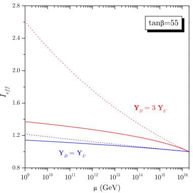
At this point few remarks are in order. First, as it has already been noticed by several authors [21], the parameter Iτ1similar-to-or-equalssubscript𝐼𝜏1I_{\tau}\simeq 1. This can be easily checked by using either the exact expression (69) or the approximate expression given in Eq. (83). Moreover, the parameter Ieffsubscript𝐼𝑒𝑓𝑓I_{eff}, which controls the RGE effects of the Dirac neutrino Yukawa coupling ratios (cf. Eq. (77)), is also close to the unity. This can be seen from Fig. 1 where we present the dependence of Ieffsubscript𝐼𝑒𝑓𝑓I_{eff} on the value of the scale μ𝜇\mu for the two initial conditions Yν=YUsubscriptY𝜈subscriptY𝑈\textbf{Y}_{\nu}=\textbf{Y}_{U} and Yν=3YUsubscriptY𝜈3subscriptY𝑈\textbf{Y}_{\nu}=3\,\textbf{Y}_{U}. We note that Ieff1similar-to-or-equalssubscript𝐼𝑒𝑓𝑓1I_{eff}\simeq 1 for a wide range of tanβ𝛽\tan\beta. Notice also that for the case Yν=3YUsubscriptY𝜈3subscriptY𝑈\textbf{Y}_{\nu}=3\,\textbf{Y}_{U}, the use of the approximate expression for Ieffsubscript𝐼𝑒𝑓𝑓I_{eff}, obtained by neglecting the running of the Yukawa couplings, is not well justified. This is because in the latter case y3(ΛX)=3yt(ΛX)subscript𝑦3subscriptΛ𝑋3subscript𝑦𝑡subscriptΛ𝑋y_{3}(\Lambda_{X})=3y_{t}(\Lambda_{X}) and the evolution of the couplings becomes more relevant.
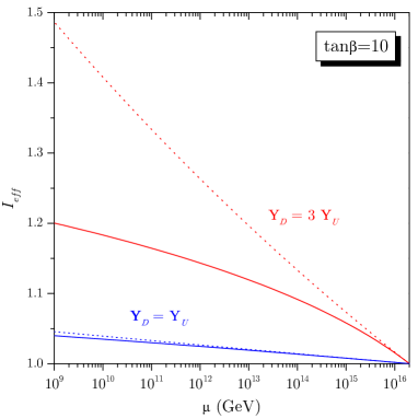
Figure 1: The evolution of the RGE coefficient Ieff=IRIν1subscript𝐼𝑒𝑓𝑓subscript𝐼𝑅superscriptsubscript𝐼𝜈1I_{eff}=I_{R}\,I_{\nu}^{-1} from ΛXsubscriptΛ𝑋\Lambda_{X} to ΛRsubscriptΛ𝑅\Lambda_{R}\ , assuming two different Dirac neutrino textures, YD=YUsubscriptY𝐷subscriptY𝑈\textbf{Y}_{D}=\textbf{Y}_{U} and YD=3YUsubscriptY𝐷3subscriptY𝑈\textbf{Y}_{D}=3\textbf{Y}_{U}\ , and for the values of tanβ=10𝛽10\tan\beta=10 and tanβ=55𝛽55\tan\beta=55. The solid curves correspond to the exact expressions as defined by Eqs. (27) and (40). The dashed lines correspond to the approximate curves as given in Eqs. (83).
Refer to caption Refer to caption

4 Confronting the neutrino mass matrix with the experimental data

The analysis of the neutrino oscillation data indicates that, contrary to what happens in the quark sector, where the mixing is always small, the mixing angle is large in the 2-3 neutrino sector. The latest atmospheric neutrino data from the Super-Kamiokande Collaboration [1] and CHOOZ experiments [2] implies a large mixing angle θatmπ/4similar-to-or-equalssubscript𝜃atm𝜋4\theta_{\text{atm}}\simeq\pi/4. In what concerns the 1-2 neutrino sector, there are four different scenarios depending on the solar neutrino problem solution.

Since the present experimental data constrains the neutrino mass squared differences and the mixing angles, it is necessary to diagonalize the effective neutrino mass matrix 𝐌νeffsuperscriptsubscript𝐌𝜈eff{\rm\bf M}_{\nu}^{\rm eff} at the electroweak scale. The neutrino mixing matrix U, which relates the flavour and mass eigenstates,

(νeνμντ)=U(ν1ν2ν3),subscript𝜈𝑒subscript𝜈𝜇subscript𝜈𝜏Usubscript𝜈1subscript𝜈2subscript𝜈3\displaystyle\left(\begin{array}[]{c}\nu_{e}\\ \nu_{\mu}\\ \nu_{\tau}\end{array}\right)=\textbf{U}\left(\begin{array}[]{c}\nu_{1}\\ \nu_{2}\\ \nu_{3}\end{array}\right)\ , (92)

can be parametrized in the standard form [25]

U=(c13c12s12c13s13s12c23s23s13c12c23c12s23s13s12s23c13s23s12s13c23c12s23c12s13s12c23c23c13),Usubscript𝑐13subscript𝑐12subscript𝑠12subscript𝑐13subscript𝑠13subscript𝑠12subscript𝑐23subscript𝑠23subscript𝑠13subscript𝑐12subscript𝑐23subscript𝑐12subscript𝑠23subscript𝑠13subscript𝑠12subscript𝑠23subscript𝑐13subscript𝑠23subscript𝑠12subscript𝑠13subscript𝑐23subscript𝑐12subscript𝑠23subscript𝑐12subscript𝑠13subscript𝑠12subscript𝑐23subscript𝑐23subscript𝑐13\displaystyle\textbf{U}=\left(\begin{array}[]{ccc}c_{13}c_{12}&s_{12}c_{13}&s_{13}\\ -s_{12}c_{23}-s_{23}s_{13}c_{12}&\quad c_{23}c_{12}-s_{23}s_{13}s_{12}&s_{23}c_{13}\\ s_{23}s_{12}-s_{13}c_{23}c_{12}&-s_{23}c_{12}-s_{13}s_{12}c_{23}&c_{23}c_{13}\end{array}\right)\ , (96)

such that UT𝐌νeff(MZ)U=diag(m1,m2,m3)superscriptU𝑇superscriptsubscript𝐌𝜈effsubscript𝑀𝑍Udiagsubscript𝑚1subscript𝑚2subscript𝑚3\textbf{U}^{T}\,{\rm\bf M}_{\nu}^{\rm eff}(M_{Z})\,\textbf{U}=\text{diag}(\,m_{1}\ ,m_{2}\ ,m_{3}\,), where misubscript𝑚𝑖m_{i} are the light neutrino masses; cijcosθij,sijsinθijformulae-sequencesubscript𝑐𝑖𝑗subscript𝜃𝑖𝑗subscript𝑠𝑖𝑗subscript𝜃𝑖𝑗c_{ij}\equiv\cos\theta_{ij}\ ,\ s_{ij}\equiv\sin\theta_{ij}\ .

We also remark that the lepton mixing matrix can have, besides a Dirac-type phase (analogous to that of the quark sector), two other physical phases associated with the Majorana character of neutrinos. If CP𝐶𝑃CP is conserved these phases are either 0 or π𝜋\pi. In the analysis that follows we shall assume all these phases vanishing. However, as we shall see in Section 4.2, such phases play a significant role in processes such as the neutrinoless double β𝛽\beta decay [26].

4.1 Neutrino oscillation data

The relevant parameter set for the study of solar and atmospheric data is usually identified with the quantities

Δm2Δm122=m22m12,Δmatm2Δm232=m32m22,formulae-sequenceΔsubscriptsuperscript𝑚2direct-productΔsubscriptsuperscript𝑚212subscriptsuperscript𝑚22subscriptsuperscript𝑚21Δsubscriptsuperscript𝑚2atmΔsubscriptsuperscript𝑚223subscriptsuperscript𝑚23subscriptsuperscript𝑚22\displaystyle\Delta m^{2}_{\odot}\equiv\Delta m^{2}_{12}=m^{2}_{2}-m^{2}_{1}\ ,\quad\Delta m^{2}_{\text{atm}}\equiv\Delta m^{2}_{23}=m^{2}_{3}-m^{2}_{2}\ ,
tan2θtan2θ12,tan2θatmtan2θ23,Ue3sinθ13,formulae-sequencesuperscript2subscript𝜃direct-productsuperscript2subscript𝜃12formulae-sequencesuperscript2subscript𝜃atmsuperscript2subscript𝜃23subscript𝑈𝑒3subscript𝜃13\displaystyle\tan^{2}\theta_{\odot}\equiv\tan^{2}\theta_{12}\ ,\quad\tan^{2}\theta_{\text{atm}}\equiv\tan^{2}\theta_{23}\ ,\quad U_{e3}\equiv\sin\theta_{13}\ , (97)

where all mixing angles are assumed to lie in the range [0,π/2]0𝜋2[0,\pi/2]. In Table 1 we summarize the present constraints on neutrino mass squared differences and on the mixing angles obtained from the recent global analyses [27, 28] of the solar, atmospheric and reactor neutrino data at 99% C.L. [90% C.L.] .

Table 1: Constraints on neutrino masses and mixing angles at 99% C.L. [90% C.L.] coming from global analyses of the solar, atmospheric and reactor neutrino data [27, 28]. The numbers in bold correspond to the best-fit values.
Atmospheric and reactor neutrinos
Δmatm2(eV2)Δsubscriptsuperscript𝑚2atmsuperscripteV2\Delta m^{2}_{\text{atm}}~{}(\text{eV}^{2}) tan2θatmsuperscript2subscript𝜃atm\tan^{2}\theta_{\text{atm}} |Ue3|subscript𝑈𝑒3|U_{e3}|
( 1.17.3)×1031.17.3superscript103(\,1.1-7.3\,){\times}10^{-3} 0.3 - 3.8 <0.27absent0.27<0.27
[ 1.46.1]×103delimited-[]1.46.1superscript103[\,1.4-6.1\,]{\times}10^{-3} [ 0.4 - 3.1 ] [<0.23]delimited-[]absent0.23[\,<0.23\,]
3.1×𝟏𝟎𝟑3.1superscript103\mathbf{3.1\times 10^{-3}} 1.4 0.07
Solar neutrinos
Δm2(eV2)Δsubscriptsuperscript𝑚2direct-productsuperscripteV2\Delta m^{2}_{\odot}~{}(\text{eV}^{2}) tan2θsuperscript2subscript𝜃direct-product\tan^{2}\theta_{\odot} r=Δm2/Δmatm2subscript𝑟direct-productΔsubscriptsuperscript𝑚2direct-productΔsubscriptsuperscript𝑚2atmr_{\odot}=\Delta m^{2}_{\odot}/\Delta m^{2}_{\text{atm}}
LMA ( 2.020)×1052.020superscript105(\,2.0-20\,){\times}10^{-5} 0.1 - 0.7 ( 0.031.8)×1010.031.8superscript101(\,0.03-1.8\,){\times}10^{-1}
[ 2.310]×105delimited-[]2.310superscript105[\,2.3-10\,]{\times}10^{-5} [ 0.2 - 0.5 ] [ 0.040.7]×101delimited-[]0.040.7superscript101[\,0.04-0.7\,]{\times}10^{-1}
4.2×𝟏𝟎𝟓4.2superscript105\mathbf{4.2\times 10^{-5}} 0.26 0.014
SMA ( 0.41)×1050.41superscript105(\,0.4-1\,){\times}10^{-5} ( 0.22)×1030.22superscript103(\,0.2-2\,){\times}10^{-3} ( 0.559.1)×1030.559.1superscript103(\,0.55-9.1\,){\times}10^{-3}
LOW ( 0.52)×1070.52superscript107(\,0.5-2\,){\times}10^{-7} 0.50.90.50.90.5-0.9 ( 0.071.8)×1040.071.8superscript104(\,0.07-1.8\,){\times}10^{-4}
Just-So2 ( 58)×101258superscript1012(\,5-8\,){\times}10^{-12} 0.520.520.5-2 ( 0.687.3)×1090.687.3superscript109(\,0.68-7.3\,){\times}10^{-9}

Apart from the overall factor Keff/ΛRsubscript𝐾𝑒𝑓𝑓subscriptΛ𝑅K_{eff}/\Lambda_{R}\,, the effective neutrino operator 𝜿(MZ)𝜿subscript𝑀𝑍\boldsymbol{\kappa}(M_{Z}) defined in Eq.(82) depends on the angles θ𝜃\theta and ϕitalic-ϕ\phi, which parametrize the heavy right-handed neutrinos, and the parameters δ1, 2subscript𝛿12\delta_{1,\,2}. For the structure of 𝜿𝜿\boldsymbol{\kappa} to be compatible with the low-energy data, we should take into account not only all the constraints on r=Δm2/Δmatm2subscript𝑟direct-productΔsubscriptsuperscript𝑚2direct-productΔsubscriptsuperscript𝑚2atmr_{\odot}=\Delta m^{2}_{\odot}/\Delta m^{2}_{\text{atm}} and the mixing angles, but also the experimentally allowed region for the up-quark mass ratios, since within our assumptions, these ratios fix the parameters δ1subscript𝛿1\delta_{1} and δ2subscript𝛿2\delta_{2} at ΛXsubscriptΛ𝑋\Lambda_{X}:

δ1ϵ1=yu(ΛX)yt(ΛX),δ2ϵ2=yc(ΛX)yt(ΛX).formulae-sequencesimilar-to-or-equalssubscript𝛿1subscriptitalic-ϵ1subscript𝑦𝑢subscriptΛ𝑋subscript𝑦𝑡subscriptΛ𝑋similar-to-or-equalssubscript𝛿2subscriptitalic-ϵ2subscript𝑦𝑐subscriptΛ𝑋subscript𝑦𝑡subscriptΛ𝑋\displaystyle\delta_{1}\simeq\epsilon_{1}=\frac{y_{u}(\Lambda_{X})}{y_{t}(\Lambda_{X})}\ ,\quad\delta_{2}\simeq\epsilon_{2}=\frac{y_{c}(\Lambda_{X})}{y_{t}(\Lambda_{X})}\ . (98)

The above ratios can be determined by running the RGE from the electroweak scale MZsubscript𝑀𝑍M_{Z} to the unification scale ΛXsubscriptΛ𝑋\Lambda_{X}, which we assume to be ΛX2×1016similar-to-or-equalssubscriptΛ𝑋2superscript1016\Lambda_{X}\simeq 2{\times}10^{16}. Since these ratios are quite insensitive to the value of tanβ𝛽\tan\beta in a wide region, we shall take tanβ=10𝛽10\tan\beta=10 as the input value in our analysis. Using the experimentally allowed values for the quark masses at the electroweak scale [29, 25], the following ranges are then obtained at ΛXsubscriptΛ𝑋\Lambda_{X}:

2.8×1062.8superscript106\displaystyle 2.8{\times}10^{-6} δ11.5×10⁵,less-than-or-similar-toabsentsubscript𝛿1less-than-or-similar-to1.5superscript105\displaystyle\lesssim\delta_{1}\lesssim 1.5{\times}10^{-5}\ ,
9×1049superscript104\displaystyle 9{\times}10^{-4} δ24×103.less-than-or-similar-toabsentsubscript𝛿2less-than-or-similar-to4superscript103\displaystyle\lesssim\delta_{2}\lesssim 4{\times}10^{-3}\ . (99)

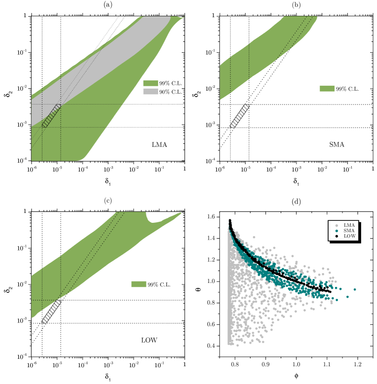
In our numerical study we randomly varied all the parameters in the ranges: 0δ1, 21, 0θπ/2, 0ϕπ/2.formulae-sequence0subscript𝛿121 0𝜃𝜋2 0italic-ϕ𝜋20\leq\delta_{1,\,2}\leq 1\ ,\ 0\leq\theta\leq\pi/2\ ,\ 0\leq\phi\leq\pi/2\ . In Fig. 2 we plot the allowed region in the plane (δ1,δ2subscript𝛿1subscript𝛿2\delta_{1},\delta_{2}) for the three different MSW solar solutions (LMA, SMA, LOW) at 99% C.L. . We assume that the right-handed Majorana neutrinos are exactly degenerate at the unification scale ΛXsubscriptΛ𝑋\Lambda_{X}. The dashed area delimited by the dotted lines corresponds to the allowed region for the Dirac neutrino coupling ratios, as defined by Eqs. (99) and assuming YνYUproportional-tosubscriptY𝜈subscriptY𝑈\textbf{Y}_{\nu}\propto\textbf{Y}_{U} at ΛXsubscriptΛ𝑋\Lambda_{X}. The intersection of the filled areas with the dashed area provides us with the points (δ1,δ2subscript𝛿1subscript𝛿2\delta_{1},\delta_{2}) compatible with the low-energy data and the initial conditions imposed at ΛXsubscriptΛ𝑋\Lambda_{X}. From the plots it is clear that the SMA solution is excluded. The LOW solution is barely compatible with the data at 99% C.L., and certainly excluded at 90% C.L. . Finally, the LMA solution is the most favoured one, and at 90% C.L. it is the only one that survives.

The results in the parameter space (ϕ,θitalic-ϕ𝜃\phi,\theta) are shown in Fig. 2d at 99% C.L. . We notice that the allowed region for LMA is more extensive than the SMA and LOW regions, and the SMA region is in turn wider than the LOW one. This is a direct consequence of the hierarchy rLMA>rSMA>rLOWsuperscriptsubscript𝑟direct-productLMAsuperscriptsubscript𝑟direct-productSMAsuperscriptsubscript𝑟direct-productLOW{r_{\odot}}^{\text{LMA}}>{r_{\odot}}^{\text{SMA}}>{r_{\odot}}^{\text{LOW}}. For the VO (Just-So2) solar solutions an extreme fine-tuning is required between θ𝜃\theta and ϕitalic-ϕ\phi in order to get a solution compatible with the solar and atmospheric neutrino data. The latter solutions are therefore not presented in our plots.

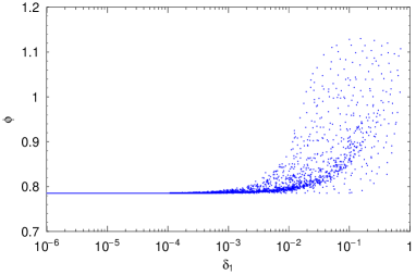
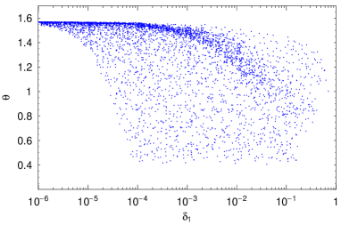
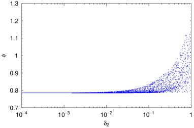
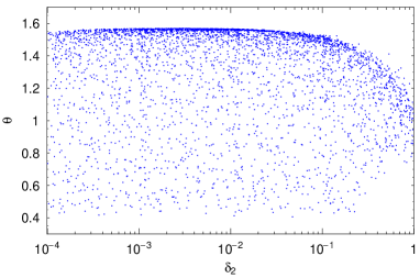
Since the LMA solution is the most favoured in the present framework, the rest of our discussion will be devoted to it. In Figs. 3 we show the allowed region at 99% C.L. for the LMA MSW solution, in different planes of the input parameters δ1,δ2,ϕsubscript𝛿1subscript𝛿2italic-ϕ\delta_{1},\delta_{2},\phi and θ𝜃\theta. A remarkable feature is the fact that for small values of δ1subscript𝛿1\delta_{1} and δ2subscript𝛿2\delta_{2}, which are required in our framework, one has ϕπ/4similar-to-or-equalsitalic-ϕ𝜋4\phi\simeq\pi/4 and θπ/2similar-to-or-equals𝜃𝜋2\theta\simeq\pi/2. We remark that the same conclusion for the value of ϕitalic-ϕ\phi can be drawn by looking at the structure of the effective neutrino mass matrix (82), since for small values of δ1, 2subscript𝛿12\delta_{1,\,2}\ , the relation cos2ϕ1much-less-than2italic-ϕ1\cos 2\phi\ll 1 is required to avoid a quasi-diagonal pattern in the mass matrix.

Let us conclude this section by giving few numerical examples (see Table 2). We consider two different GUT-motivated relations for the Dirac neutrino Yukawa coupling matrix: Yν=YUsubscriptY𝜈subscriptY𝑈\textbf{Y}_{\nu}=\textbf{Y}_{U} and Yν=3YUsubscriptY𝜈3subscriptY𝑈\textbf{Y}_{\nu}=3\textbf{Y}_{U}. In both cases, consistency with the present LMA solar, atmospheric and reactor neutrino data was achieved. It was not possible however to obtain the best-fit values, simultaneously for all the parameters. By slightly modifying the initial assumption y1/y3=yu/ytsubscript𝑦1subscript𝑦3subscript𝑦𝑢subscript𝑦𝑡y_{1}/y_{3}=y_{u}/y_{t}\ , we were then able to reproduce the best-fit values for all the solar and atmospheric neutrino data, as shown in the last column of the table. Notice also that the obtained value |Ue3|0.05similar-to-or-equalssubscript𝑈𝑒30.05|U_{e3}|\simeq 0.05 is close to the best-fit value |Ue3|=0.07subscript𝑈𝑒30.07|U_{e3}|=0.07 given in Table 1.

As suggested by our full numerical analysis (see Figs. 3), the angles θ𝜃\theta and ϕitalic-ϕ\phi were chosen to be close to π/2𝜋2\pi/2 and π/4𝜋4\pi/4, respectively. The degeneracy imposed at ΛXsubscriptΛ𝑋\Lambda_{X} for the right-handed Majorana neutrinos, |M1|=|M2|=|M3|subscript𝑀1subscript𝑀2subscript𝑀3|M_{1}|=|M_{2}|=|M_{3}|\ , is lifted in all cases by radiative corrections. At the decoupling scale ΛRsubscriptΛ𝑅\Lambda_{R} we have |M1||M2|IRΛR<|M3|ΛRsimilar-to-or-equalssubscript𝑀1subscript𝑀2similar-to-or-equalssubscript𝐼𝑅subscriptΛ𝑅subscript𝑀3similar-to-or-equalssubscriptΛ𝑅|M_{1}|\simeq|M_{2}|\simeq I_{R}\Lambda_{R}<|M_{3}|\simeq\Lambda_{R}. For the effective neutrinos with masses misubscript𝑚𝑖m_{i}\ , we obtain at the electroweak scale a hierarchical spectrum with

|m1|<|m2|Δm122<|m3|Δm232.subscript𝑚1subscript𝑚2similar-to-or-equalsΔsubscriptsuperscript𝑚212subscript𝑚3similar-to-or-equalsΔsubscriptsuperscript𝑚223\displaystyle|m_{1}|<|m_{2}|\simeq\sqrt{\Delta m^{2}_{12}}<|m_{3}|\simeq\sqrt{\Delta m^{2}_{23}}\ . (100)

Finally, we also notice the stability of the atmospheric and solar neutrino parameters, rν=Δm122/Δm232,tan2θ12,tan2θ23subscript𝑟𝜈Δsubscriptsuperscript𝑚212Δsubscriptsuperscript𝑚223superscript2subscript𝜃12superscript2subscript𝜃23r_{\nu}=\Delta m^{2}_{12}/\Delta m^{2}_{23}\ ,\ \tan^{2}\theta_{12}\ ,\ \tan^{2}\theta_{23} and Ue3subscript𝑈𝑒3U_{e3} with the energy scale. In fact, from ΛRsubscriptΛ𝑅\Lambda_{R} to MZsubscript𝑀𝑍M_{Z} no significant running of these parameters is observed. This is related with the fact that Iτ1similar-to-or-equalssubscript𝐼𝜏1I_{\tau}\simeq 1.

Figure 2: Allowed region in the plane (δ1,δ2subscript𝛿1subscript𝛿2\delta_{1},\delta_{2}) for the three different MSW solar solutions (LMA, SMA, LOW) at 99% C.L., if we assume YνYUproportional-tosubscriptY𝜈subscriptY𝑈\textbf{Y}_{\nu}\propto\textbf{Y}_{U} and an exactly degenerate spectrum for the right-handed Majorana neutrinos at the unification scale ΛXsubscriptΛ𝑋\Lambda_{X}. The dashed area corresponds to the allowed region for the up quark mass ratios at ΛXsubscriptΛ𝑋\Lambda_{X}. At 90% C.L., the only solution that is compatible with the experimental data is the LMA one. The corresponding allowed region in the plane (ϕ,θitalic-ϕ𝜃\phi,\theta) is shown in Fig. 2d at 99% C.L. .
Refer to caption
Figure 3: Allowed region at 99% C.L. for the most favoured solar solution, namely the LMA MSW solution, in different planes of the input parameters δ1,δ2,ϕsubscript𝛿1subscript𝛿2italic-ϕ\delta_{1},\delta_{2},\phi and θ𝜃\theta, within our framework. For small values of the parameters δ1subscript𝛿1\delta_{1} and δ2subscript𝛿2\delta_{2}, the angles ϕitalic-ϕ\phi and θ𝜃\theta approach π/4𝜋4\pi/4 and π/2𝜋2\pi/2, respectively.
Refer to caption Refer to caption
Table 2: Numerical results for tanβ=10𝛽10\tan\beta=10. We assume right-handed neutrino degeneracy at ΛXsubscriptΛ𝑋\Lambda_{X}, which is then lifted by radiative corrections. Two different Ansätze were considered for the Dirac neutrino Yukawa coupling matrix, Yν=YUsubscriptY𝜈subscriptY𝑈\textbf{Y}_{\nu}=\textbf{Y}_{U} and Yν=3YUsubscriptY𝜈3subscriptY𝑈\textbf{Y}_{\nu}=3\textbf{Y}_{U}. By slightly modifying the initial condition y1/y3=yu/ytsubscript𝑦1subscript𝑦3subscript𝑦𝑢subscript𝑦𝑡y_{1}/y_{3}=y_{u}/y_{t} it is possible to reproduce the best-fit values for all the solar and atmospheric neutrino data, as shown in the last column of the table. The negative CP𝐶𝑃CP parities are indicated by ()(-).
Yν=YUsubscriptY𝜈subscriptY𝑈\textbf{Y}_{\nu}=\textbf{Y}_{U} Yν=3YUsubscriptY𝜈3subscriptY𝑈\textbf{Y}_{\nu}=3\,\textbf{Y}_{U} Best fit
At ΛX=2.0×10¹⁶subscriptΛ𝑋2.0superscript1016\Lambda_{X}=2.0{\times}10^{16} GeV
yusubscript𝑦𝑢y_{u} 5.0×1065.0superscript1065.0{\times}10^{-6} 5.9×1065.9superscript1065.9{\times}10^{-6} 5.6×1065.6superscript1065.6{\times}10^{-6}
ycsubscript𝑦𝑐y_{c} 1.7×1031.7superscript1031.7{\times}10^{-3} 2.1×1032.1superscript1032.1{\times}10^{-3} 1.7×1031.7superscript1031.7{\times}10^{-3}
ytsubscript𝑦𝑡y_{t} 0.68 0.80 0.64
y1subscript𝑦1y_{1} 5.0×1065.0superscript1065.0{\times}10^{-6} 1.8×1051.8superscript1051.8{\times}10^{-5} 6.4×1076.4superscript1076.4{\times}10^{-7}
y2subscript𝑦2y_{2} 1.7×1031.7superscript1031.7{\times}10^{-3} 6.3×1036.3superscript1036.3{\times}10^{-3} 1.7×1031.7superscript1031.7{\times}10^{-3}
y3subscript𝑦3y_{3} 0.68 2.4 0.64
π/2θ𝜋2𝜃\pi/2-\theta 7.0×1037.0superscript1037.0{\times}10^{-3} 7.0×1037.0superscript1037.0{\times}10^{-3} 2.6×1032.6superscript1032.6{\times}10^{-3}
ϕπ/4italic-ϕ𝜋4\phi-\pi/4 1.0×1051.0superscript1051.0{\times}10^{-5} 1.0×1051.0superscript1051.0{\times}10^{-5} 2.3×1062.3superscript1062.3{\times}10^{-6}
At ΛR=subscriptΛ𝑅absent\Lambda_{R}\,= 2.6×1092.6superscript1092.6{\times}10^{9} GeV 1.4×10111.4superscript10111.4{\times}10^{11} GeV 6.3×1086.3superscript1086.3{\times}10^{8} GeV
M1subscript𝑀1M_{1} (GeV) 2.4×1092.4superscript1092.4{\times}10^{9} 9.6×10109.6superscript10109.6{\times}10^{10} 5.8×1085.8superscript1085.8{\times}10^{8}
M2subscript𝑀2M_{2} (GeV) () 2.4×1092.4superscript109(-)\,2.4{\times}10^{9} () 9.6×10109.6superscript1010(-)\,9.6{\times}10^{10} () 5.8×1085.8superscript108(-)\,5.8{\times}10^{8}
M3subscript𝑀3M_{3} (GeV) 2.6×1092.6superscript1092.6{\times}10^{9} 1.4×10111.4superscript10111.4{\times}10^{11} 6.3×1086.3superscript1086.3{\times}10^{8}
rνsubscript𝑟𝜈r_{\nu} 6.7×1026.7superscript1026.7{\times}10^{-2} 8.1×1028.1superscript1028.1{\times}10^{-2} 1.4×1021.4superscript1021.4{\times}10^{-2}
tan2θ12superscript2subscript𝜃12\tan^{2}\theta_{12} 0.34 0.34 0.26
tan2θ23superscript2subscript𝜃23\tan^{2}\theta_{23} 0.47 0.57 1.4
|Ue3|subscript𝑈𝑒3|U_{e3}| 0.18 0.18 0.05
At MZ=91.2subscript𝑀𝑍91.2M_{Z}=91.2 GeV
Keffsubscript𝐾𝑒𝑓𝑓K_{eff} 0.31 2.18 0.30
m1subscript𝑚1m_{1} (eV) 1.6×1031.6superscript1031.6{\times}10^{-3} 1.9×1031.9superscript1031.9{\times}10^{-3} 1.6×1031.6superscript1031.6{\times}10^{-3}
m2subscript𝑚2m_{2} (eV) () 1.0×1021.0superscript102(-)\,1.0{\times}10^{-2} () 1.1×1021.1superscript102(-)\,1.1{\times}10^{-2} () 6.8×1036.8superscript103(-)\,6.8{\times}10^{-3}
m3subscript𝑚3m_{3} (eV) 4.0×1024.0superscript1024.0{\times}10^{-2} 3.9×1023.9superscript1023.9{\times}10^{-2} 5.6×1025.6superscript1025.6{\times}10^{-2}
Δm122(eV2)Δsubscriptsuperscript𝑚212superscripteV2\Delta m^{2}_{12}~{}(\text{eV}^{2}) 1.0×1041.0superscript1041.0{\times}10^{-4} 1.2×1041.2superscript1041.2{\times}10^{-4} 4.3×1054.3superscript1054.3{\times}10^{-5}
Δm232(eV2)Δsubscriptsuperscript𝑚223superscripteV2\Delta m^{2}_{23}~{}(\text{eV}^{2}) 1.5×1031.5superscript1031.5{\times}10^{-3} 1.4×1031.4superscript1031.4{\times}10^{-3} 3.1×1033.1superscript1033.1{\times}10^{-3}
rνsubscript𝑟𝜈r_{\nu} 6.7×1026.7superscript1026.7{\times}10^{-2} 8.1×1028.1superscript1028.1{\times}10^{-2} 1.4×1021.4superscript1021.4{\times}10^{-2}
tan2θ12superscript2subscript𝜃12\tan^{2}\theta_{12} 0.34 0.34 0.26
tan2θ23superscript2subscript𝜃23\tan^{2}\theta_{23} 0.47 0.57 1.4
|Ue3|subscript𝑈𝑒3|U_{e3}| 0.18 0.18 0.05
|<m>|expectation𝑚\left|<\!m\!>\right|\  (eV) 2.0×10122.0superscript10122.0{\times}10^{-12} 2.4×10122.4superscript10122.4{\times}10^{-12} 9.8×10159.8superscript10159.8{\times}10^{-15}
musubscript𝑚𝑢m_{u} (MeV) 1.9 2.0 2.2
mcsubscript𝑚𝑐m_{c} (GeV) 0.68 0.69 0.66
mtsubscript𝑚𝑡m_{t} (GeV) 174 174 175
Down-quark masses md=4.61subscript𝑚𝑑4.61m_{d}=4.61 MeV ms=91.8subscript𝑚𝑠91.8m_{s}=91.8 MeV mb=2.99subscript𝑚𝑏2.99m_{b}=2.99 GeV
Charged-lepton masses me=0.49subscript𝑚𝑒0.49m_{e}=0.49 MeV mμ=102.8subscript𝑚𝜇102.8m_{\mu}=102.8 MeV mτ=1.75subscript𝑚𝜏1.75m_{\tau}=1.75 GeV

4.2 Neutrinoless double 𝜷𝜷\boldsymbol{\beta} decay

The Majorana nature of massive neutrinos can be traced by looking for processes where the total lepton charge L𝐿L changes by two units, i.e. ΔL=2Δ𝐿2\Delta L=2. The information coming from these type of events can be crucial not only to establish the nature of neutrinos but also to reveal some aspects about CP𝐶𝑃CP violation in the leptonic sector, to which neutrino oscillations are insensitive. In particular, if neutrinos have a Dirac signature, then the two extra Majorana phases which appear in the neutrino mixing matrix will be absent. Moreover, even if CP𝐶𝑃CP invariance holds, some information about the relative CP𝐶𝑃CP parities and neutrino mass spectrum can be extracted. One example of such processes is the neutrinoless double β𝛽\beta decay (ββ0ν𝛽subscript𝛽0𝜈\beta\beta_{0\nu}\,- decay) of the type

(A,Z)(A,Z+2)+2e,𝐴𝑍𝐴𝑍22superscript𝑒\displaystyle(A,Z)\rightarrow(A,Z+2)+2\,e^{-}\,, (101)

which can occur through the exchange of massive Majorana neutrinos coupled to electrons. The decay rate is proportional to the so-called “effective Majorana mass parameter”

|<m>|=|m1Ue1 2+m2Ue2 2+m3Ue3 2|.expectation𝑚subscript𝑚1superscriptsubscript𝑈𝑒12subscript𝑚2superscriptsubscript𝑈𝑒22subscript𝑚3superscriptsubscript𝑈𝑒32\displaystyle\mbox{$\left|<\!m\!>\right|\ $}=\left|m_{1}\,U_{e1}^{\,2}+m_{2}\,U_{e2}^{\,2}+m_{3}\,U_{e3}^{\,2}\right|\,. (102)

Although no experimental evidence has been found so far for this kind of processes, an upper bound has been obtained by the Ge76superscriptGe76{}^{76}{\rm Ge} Heidelberg-Moscow experiment [30]:

|<m>|<0.35eV[ 90%C.L.].\displaystyle\mbox{$\left|<\!m\!>\right|\ $}<0.35~{}\text{eV}\;[\,90\%\,{\rm C.L.}\,]\,. (103)

If CP𝐶𝑃CP is conserved, then Eq. (102) can be written as

|<m>|=|η1CPm1Ue1 2+η2CPm2Ue2 2+η3CPm3Ue3 2|,mi>0,formulae-sequenceexpectation𝑚superscriptsubscript𝜂1𝐶𝑃subscript𝑚1superscriptsubscript𝑈𝑒12superscriptsubscript𝜂2𝐶𝑃subscript𝑚2superscriptsubscript𝑈𝑒22superscriptsubscript𝜂3𝐶𝑃subscript𝑚3superscriptsubscript𝑈𝑒32subscript𝑚𝑖0\displaystyle\mbox{$\left|<\!m\!>\right|\ $}=\left|\eta_{1}^{CP}m_{1}\,U_{e1}^{\,2}+\eta_{2}^{CP}\,m_{2}\,U_{e2}^{\,2}+\eta_{3}^{CP}\,m_{3}\,U_{e3}^{\,2}\right|\ ,\quad m_{i}>0\ , (104)

where ηiCP=±1superscriptsubscript𝜂𝑖𝐶𝑃plus-or-minus1\eta_{i}^{CP}={\pm}1 are the neutrino CP𝐶𝑃CP parities. By examining the invariants of the effective neutrino mass matrix given in Eq. (82), one can conclude that one of the neutrinos should have a negative CP𝐶𝑃CP parity and the other two should have positive CP𝐶𝑃CP parity. This is verified for the numerical examples considered in Table 2, where the neutrino with mass m2subscript𝑚2m_{2} has η2CP=1superscriptsubscript𝜂2𝐶𝑃1\eta_{2}^{CP}=-1, while the other two have η1,3CP=+1superscriptsubscript𝜂13𝐶𝑃1\eta_{1,3}^{CP}=+1. In this case, Eq. (104) reads

|<m>|=|m1Ue1 2m2Ue2 2+m3Ue3 2|.expectation𝑚subscript𝑚1superscriptsubscript𝑈𝑒12subscript𝑚2superscriptsubscript𝑈𝑒22subscript𝑚3superscriptsubscript𝑈𝑒32\displaystyle\mbox{$\left|<\!m\!>\right|\ $}=\left|m_{1}\,U_{e1}^{\,2}-m_{2}\,U_{e2}^{\,2}+m_{3}\,U_{e3}^{\,2}\right|\ . (105)

A particular feature in the above expression is the possibility of a cancellation among the different terms [31, 26], such that |<m>|0similar-to-or-equalsexpectation𝑚0\mbox{$\left|<\!m\!>\right|\ $}\simeq 0. In fact, for all the numerical cases considered in Table 2, such a cancellation indeed occurs. This can be easily understood if we recall that the effective Majorana mass parameter is nothing but the absolute value of (𝐌νeff)11subscriptsuperscriptsubscript𝐌𝜈eff11({\rm\bf M}_{\nu}^{\rm eff})_{11}. Therefore, from Eq. (82) we have

|<m>||δ12(cθ2+c2ϕsθ2)|.proportional-toexpectation𝑚superscriptsubscript𝛿12subscriptsuperscript𝑐2𝜃subscript𝑐2italic-ϕsubscriptsuperscript𝑠2𝜃\displaystyle\mbox{$\left|<\!m\!>\right|\ $}\propto|\,\delta_{1}^{2}\,(c^{2}_{\theta}+c_{2\phi}\,s^{2}_{\theta})\,|\,. (106)

Since θπ/2similar-to-or-equals𝜃𝜋2\theta\simeq\pi/2 and ϕπ/4similar-to-or-equalsitalic-ϕ𝜋4\phi\simeq\pi/4, in order to account for the low-energy neutrino data, and δ1subscript𝛿1\delta_{1} is small, it is now clear from Eq. (106) why |<m>|expectation𝑚\left|<\!m\!>\right|\ is highly suppressed in our framework.

5 A simple analytical form for 𝐌νeffsuperscriptsubscript𝐌𝜈eff{\rm\bf M}_{\nu}^{\rm eff}

In this section we shall present a simple analytical example which can reproduce the results obtained in the last section. We have seen that, in the context of complete degeneracy of right-handed neutrinos and imposing proportionality between YνsubscriptY𝜈\textbf{Y}_{\nu} and YUsubscriptY𝑈\textbf{Y}_{U}, the only possible solution at low energies is the LMA. Moreover, as it is clear from Figs. 3 this would require θπ/2similar-to-or-equals𝜃𝜋2\theta\simeq\pi/2 and ϕπ/4similar-to-or-equalsitalic-ϕ𝜋4\phi\simeq\pi/4. On the other hand, if one assumes in Eq. (82), ϕ=π/4italic-ϕ𝜋4\phi=\pi/4 and θ=π/2𝜃𝜋2\theta=\pi/2, then

𝜿(MZ)=KeffΛR(00δ10δ220δ100).𝜿subscript𝑀𝑍subscript𝐾𝑒𝑓𝑓subscriptΛ𝑅00subscript𝛿10superscriptsubscript𝛿220subscript𝛿100\displaystyle\boldsymbol{\kappa}(M_{Z})=\frac{K_{eff}}{\Lambda_{R}}\left(\begin{array}[]{ccc}0&0&-\delta_{1}\\ 0&\delta_{2}^{2}&0\\ -\delta_{1}&0&0\end{array}\right)\ . (110)

In this case the neutrino masses are

{m1,m2,m3}=KeffΛRv2sin2β{δ1,δ1,δ22}.subscript𝑚1subscript𝑚2subscript𝑚3subscript𝐾𝑒𝑓𝑓subscriptΛ𝑅superscript𝑣2superscript2𝛽subscript𝛿1subscript𝛿1superscriptsubscript𝛿22\displaystyle\{\,m_{1}\ ,\,m_{2}\ ,\,m_{3}\,\}=\frac{K_{eff}}{\Lambda_{R}}\,v^{2}\sin^{2}\beta\,\{\,\delta_{1}\,,\,\delta_{1}\,,\,\delta_{2}^{2}\,\}\ . (111)

Taking into account Eqs. (110) and (111), it is straightforward to show that, independently of the value of the parameters δ1subscript𝛿1\delta_{1} and δ2subscript𝛿2\delta_{2}, one always has sin2(2θ23)=0superscript22subscript𝜃230\sin^{2}(2\,\theta_{23})=0, which is not phenomenologically viable.

At first sight the above result may seem contradictory, since on one hand our numerical study clearly shows that values of θπ/2similar-to-or-equals𝜃𝜋2\theta\simeq\pi/2 and ϕπ/4similar-to-or-equalsitalic-ϕ𝜋4\phi\simeq\pi/4 are indeed compatible with the low-energy neutrino data, but on the other hand, a simple analytical check gives a completely opposite answer. As we shall see shortly, the reason for this mismatching lies in the fact that small deviations, such as δθ=π/2θ1𝛿𝜃𝜋2𝜃much-less-than1\delta\theta=\pi/2-\theta\ll 1 and δϕ=ϕπ/41𝛿italic-ϕitalic-ϕ𝜋4much-less-than1\delta\phi=\phi-\pi/4\ll 1, and/or small perturbations from our original assumptions, turn out to be crucial. To show that this is indeed the case, let us relax the condition of proportionality between YνsubscriptY𝜈\textbf{Y}_{\nu} and YUsubscriptY𝑈\textbf{Y}_{U} for the smallest Dirac neutrino Yukawa coupling by putting

ϵ1=aϵ2,ϵ2=ϵ=yc(ΛX)yt(ΛX),formulae-sequencesubscriptitalic-ϵ1𝑎superscriptitalic-ϵ2subscriptitalic-ϵ2italic-ϵsubscript𝑦𝑐subscriptΛ𝑋subscript𝑦𝑡subscriptΛ𝑋\displaystyle\epsilon_{1}=a\,\epsilon^{2}\ ,\quad\epsilon_{2}=\epsilon=\frac{y_{c}(\Lambda_{X})}{y_{t}(\Lambda_{X})}\ , (112)

and write θ𝜃\theta and ϕitalic-ϕ\phi as

ϕ=π4+bϵ2,θ=π2ϵ,formulae-sequenceitalic-ϕ𝜋4𝑏superscriptitalic-ϵ2𝜃𝜋2italic-ϵ\displaystyle\phi=\frac{\pi}{4}+b\,\epsilon^{2}\ ,\quad\theta=\frac{\pi}{2}-\epsilon\ , (113)

where a𝑎a and b𝑏b are some positive real constants. From Eq. (77) we have then

δ1=aIeffIτ1ϵ2aϵ2,δ2=IeffIτ1ϵϵ.formulae-sequencesubscript𝛿1𝑎subscript𝐼𝑒𝑓𝑓superscriptsubscript𝐼𝜏1superscriptitalic-ϵ2similar-to-or-equals𝑎superscriptitalic-ϵ2subscript𝛿2subscript𝐼𝑒𝑓𝑓superscriptsubscript𝐼𝜏1italic-ϵsimilar-to-or-equalsitalic-ϵ\displaystyle\delta_{1}=a\,I_{eff}\,I_{\tau}^{-1}\,\epsilon^{2}\simeq a\,\epsilon^{2}\ ,\quad\quad\delta_{2}=I_{eff}\,I_{\tau}^{-1}\,\epsilon\simeq\epsilon\ . (114)

The effective neutrino mass operator (82) will be approximately given in this case by

𝜿(MZ)KeffΛRϵ2(a2ϵ4( 12b)aϵ2aaϵ212bϵ41a12b).similar-to-or-equals𝜿subscript𝑀𝑍subscript𝐾𝑒𝑓𝑓subscriptΛ𝑅superscriptitalic-ϵ2superscript𝑎2superscriptitalic-ϵ412𝑏𝑎superscriptitalic-ϵ2𝑎𝑎superscriptitalic-ϵ212𝑏superscriptitalic-ϵ41𝑎12𝑏\displaystyle\boldsymbol{\kappa}(M_{Z})\simeq\frac{K_{eff}}{\Lambda_{R}}\,\epsilon^{2}\,\left(\begin{array}[]{ccc}a^{2}\,\epsilon^{4}\,(\,1-2\,b\,)&-a\,\epsilon^{2}&-a\\ -a\,\epsilon^{2}&\quad 1-2\,b\,\epsilon^{4}&-1\\ -a&-1&2\,b\end{array}\right)\ . (118)

Due to the smallness of the parameter ϵitalic-ϵ\epsilon we have, to a very good approximation,

𝜿(MZ)KeffΛRϵ2𝜿,𝜿=(00a011a12b).\displaystyle\boldsymbol{\kappa}(M_{Z})\simeq\frac{K_{eff}}{\Lambda_{R}}\,\epsilon^{2}\,\boldsymbol{\kappa}^{\prime}\quad,\quad\boldsymbol{\kappa}^{\prime}=\left(\begin{array}[]{ccc}0&0&-a\\ 0&1&-1\\ -a&-1&2\,b\end{array}\right)\ . (122)

The invariants of the matrix 𝜿superscript𝜿\boldsymbol{\kappa}^{\prime} are

T =λ1+λ2+λ3=1+2b,absentsubscript𝜆1subscript𝜆2subscript𝜆312𝑏\displaystyle=\lambda_{1}+\lambda_{2}+\lambda_{3}=1+2\,b\ ,
χ𝜒\displaystyle\chi =λ1λ2+λ1λ3+λ2λ3=1a22b,absentsubscript𝜆1subscript𝜆2subscript𝜆1subscript𝜆3subscript𝜆2subscript𝜆31superscript𝑎22𝑏\displaystyle=\lambda_{1}\,\lambda_{2}+\lambda_{1}\,\lambda_{3}+\lambda_{2}\,\lambda_{3}=-1-a^{2}-2\,b\ ,
ΔΔ\displaystyle\Delta =λ1λ2λ3=a2,absentsubscript𝜆1subscript𝜆2subscript𝜆3superscript𝑎2\displaystyle=\lambda_{1}\,\lambda_{2}\,\lambda_{3}=-a^{2}\ , (123)

where λisubscript𝜆𝑖\lambda_{i}\ are the eigenvalues,

λ1subscript𝜆1\displaystyle\lambda_{1} =2pcos(α3)+T,absent2𝑝𝛼3T\displaystyle=2\,\sqrt{p}\,\cos\left(\frac{\alpha}{3}\right)+\text{T}\ ,
λ 2, 3subscript𝜆23\displaystyle\lambda_{\,2,\,3} =2pcos(α3±π3)+T,absent2𝑝plus-or-minus𝛼3𝜋3T\displaystyle=-2\,\sqrt{p}\,\cos\left(\frac{\alpha}{3}{\pm}\frac{\pi}{3}\right)+\text{T}\ , (124)

with

q=2T 327+Tχ3Δ,p=T 29χ3,cosα=qp 3/2.formulae-sequence𝑞2superscriptT327T𝜒3Δformulae-sequence𝑝superscriptT29𝜒3𝛼𝑞superscript𝑝32\displaystyle q=-\frac{2\,\text{T}^{\,3}}{27}+\frac{\text{T}\,\chi}{3}-\Delta\ ,\quad p=\frac{\text{T}^{\,2}}{9}-\frac{\chi}{3}\ ,\quad\cos\alpha=-\frac{q}{p^{\,3/2}}\ . (125)

The corresponding eigenvectors are given by

vi=1ni[a( 1λi),λi,λi(λi1)]T,subscriptv𝑖1subscript𝑛𝑖superscript𝑎1subscript𝜆𝑖subscript𝜆𝑖subscript𝜆𝑖subscript𝜆𝑖1𝑇\displaystyle\textbf{v}_{i}=\frac{1}{n_{i}}\left[\,a\,(\,1-\lambda_{i}\,)\,,\,-\lambda_{i}\,,\,\lambda_{i}\,(\,\lambda_{i}-1\,)\,\right]^{\,T}\ , (126)

where nisubscript𝑛𝑖n_{i} are the normalization coefficients.

In Fig. 4 we present the region in the (a,b)𝑎𝑏(a,b)-plane, which is compatible with the low-energy solar and atmospheric neutrino data at 90% and 99% C.L. for the LMA solution (cf. Table 1). We see that no fine-tuning is required in order to reproduce the data. To obtain the best-fit point (black dot in the figure), we assume at the unification scale ΛXsubscriptΛ𝑋\Lambda_{X} the same values for the charm and top Yukawa couplings as in the last column of Table 2, i.e. yc(ΛX)=1.7×10³subscript𝑦𝑐subscriptΛ𝑋1.7superscript103y_{c}(\Lambda_{X})=1.7{\times}10^{-3} and yt(ΛX)=0.64subscript𝑦𝑡subscriptΛ𝑋0.64y_{t}(\Lambda_{X})=0.64\ . Taking then as input parameters

ϵ=yc(ΛX)yt(ΛX)=2.65×10³,a=0.15,b=0.34,ΛR=6.3×10⁸GeV,formulae-sequenceitalic-ϵsubscript𝑦𝑐subscriptΛ𝑋subscript𝑦𝑡subscriptΛ𝑋2.65superscript103formulae-sequence𝑎0.15formulae-sequence𝑏0.34subscriptΛ𝑅6.3superscript108GeV\displaystyle\epsilon=\frac{y_{c}(\Lambda_{X})}{y_{t}(\Lambda_{X})}=2.65{\times}10^{-3}\ ,\quad a=0.15\ ,\quad b=0.34\ ,\quad\Lambda_{R}=6.3{\times}10^{8}~{}\text{GeV}\ , (127)

the following values are obtained at the electroweak scale for tanβ=10𝛽10\tan\beta=10\ :

(133)

which correspond to the best-fit values in the neutrino mixing plane for the atmospheric neutrinos [27] and the LMA solar neutrino solution [28].
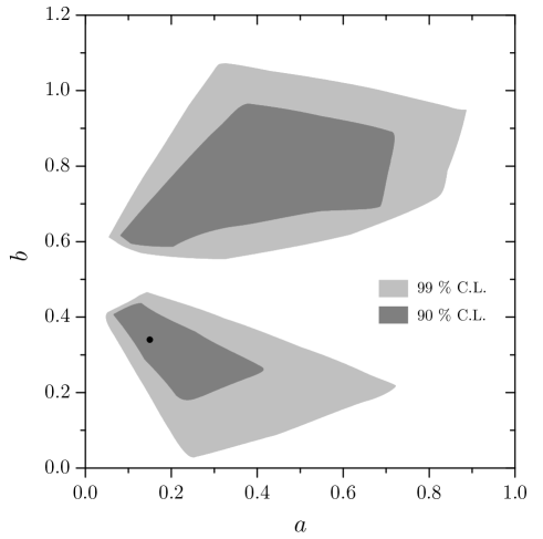
Figure 4: Allowed region for the parameters a𝑎a and b𝑏b of the triangular texture (122) for 𝜿(MZ)𝜿subscript𝑀𝑍\boldsymbol{\kappa}(M_{Z}), in the case of the LMA MSW solution and considering the neutrino data at 90% and 99% C.L. summarized in Table 1. The black dot corresponds to the point which leads to the best-fit values of the solar and atmospheric data as shown in Eqs. (127)-(133).
Refer to caption

6 Conclusions

In this paper we have considered the possibility of having an exactly degenerate spectrum for heavy right-handed Majorana neutrinos at the grand unification scale. Our theoretical framework was based on the minimal supersymmetric standard model with unbroken R𝑅R parity and extended with three heavy Majorana neutrino fields. We assumed no Dirac-type leptonic mixing at GUT scale, and thus the right-handed neutrino sector constitutes the only source of lepton flavour violation in this context. We have then studied the renormalization group effects, which include the neutrino threshold effects, from high to low energies.

Taking into account the allowed range for the quark mass ratios at GUT scale and the effective neutrino mass matrix obtained through the seesaw mechanism, we have investigated which of the possible solutions to the solar neutrino problem can be accommodated in our framework. Inspired by GUT-motivated relations among the quark, charged-lepton and Dirac neutrino mass matrices, and based on the latest global analyses of the solar and atmospheric data at 99% C.L., we have then concluded that the only solar solutions compatible with the experimental data are the LOW and LMA solutions. In fact, at 90% C.L. only the latter is allowed. Even in this case, the obtained values for the neutrino oscillation parameters are far from the best-fit points. In this sense, right-handed neutrino degeneracy embedded in GUT scenarios seems to be disfavoured by the low-energy neutrino data. We emphasize however that, by slightly relaxing the imposed relations among the Yukawa coupling matrices at high scale, one can easily reach the best-fit values. Our assumption of degeneracy is in fact a very restrictive one, since the right-handed Majorana neutrino matrix MRsubscriptM𝑅\textbf{M}_{R} is parametrized in terms of only two angles and an overall scale ΛRsubscriptΛ𝑅\Lambda_{R}. On the other hand, a fully or partially hierarchical mass spectrum for right-handed neutrinos can be easily achieved with a much less constrained structure, and one could therefore expect that such patterns are easier to be reconciled with the low-energy neutrino data.

Finally, we are also aware of possible contributions to lepton flavour violation processes like μeγ𝜇𝑒𝛾\mu\rightarrow e\gamma\,. As it has been recently pointed out by Casas and Ibarra [32], in supersymmetric theories with seesaw-like neutrino masses the prediction for the branching ratio of this process is, in general, larger than the experimental upper bound. In particular, scenarios such as the one considered here, where top-neutrino unification occurs, are severely constrained unless the leptonic Yukawa coupling matrices satisfy very specific requirements.

Acknowledgments.
We thank E.Kh. Akhmedov for a careful reading of the manuscript and useful comments. We are also grateful to D.F. Carvalho for bringing to our attention some aspects of lepton flavour violation in μeγ𝜇𝑒𝛾\mu\rightarrow e\gamma\,. The work of R.G.F. and F.R.J. has been supported by Fundação para a Ciência e a Tecnologia under the grants SFRH/BPD/1549/2000 and PRAXISXXI/BD/18219/98, respectively.

Appendix A Renormalization group equations

In this Appendix we present the relevant one-loop renormalization group equations for the MSSM extended with three right-handed Majorana neutrinos.

Between ΛXsubscriptΛ𝑋\Lambda_{X} and ΛRsubscriptΛ𝑅\Lambda_{R} the evolution of the up-quark, YUsubscriptY𝑈\textbf{Y}_{U}\,, down-quark, YDsubscriptY𝐷\textbf{Y}_{D}\,, charged-lepton, YsubscriptY\textbf{Y}_{\ell}\,, and Dirac neutrino, YνsubscriptY𝜈\textbf{Y}_{\nu}\,, Yukawa coupling matrices is given by

16π2dYUdt16superscript𝜋2𝑑subscriptY𝑈𝑑𝑡\displaystyle 16\,\pi^{2}\frac{d\textbf{Y}_{U}}{dt} =[(TUGU)+( 3YUYU+YDYD)]YU,absentdelimited-[]subscript𝑇𝑈subscript𝐺𝑈3subscriptY𝑈superscriptsubscriptY𝑈subscriptY𝐷superscriptsubscriptY𝐷subscriptY𝑈\displaystyle=\left[\,(\,T_{U}-G_{U}\,)+(\,3\,\textbf{Y}_{U}\textbf{Y}_{U}^{\dagger}+\textbf{Y}_{D}\textbf{Y}_{D}^{\dagger}\,)\,\right]\textbf{Y}_{U}\ , (134)
16π2dYDdt16superscript𝜋2𝑑subscriptY𝐷𝑑𝑡\displaystyle 16\,\pi^{2}\frac{d\textbf{Y}_{D}}{dt} =[(TDGD)+( 3YDYD+YUYU)]YD,absentdelimited-[]subscript𝑇𝐷subscript𝐺𝐷3subscriptY𝐷superscriptsubscriptY𝐷subscriptY𝑈superscriptsubscriptY𝑈subscriptY𝐷\displaystyle=\left[\,(\,T_{D}-G_{D}\,)+(\,3\,\textbf{Y}_{D}\textbf{Y}_{D}^{\dagger}+\textbf{Y}_{U}\textbf{Y}_{U}^{\dagger}\,)\,\right]\textbf{Y}_{D}\ , (135)
16π2dYdt16superscript𝜋2𝑑subscriptY𝑑𝑡\displaystyle 16\,\pi^{2}\frac{d\textbf{Y}_{\ell}}{dt} =[(TG)+( 3YY+YνYν)]Y,absentdelimited-[]subscript𝑇subscript𝐺3subscriptYsuperscriptsubscriptYsubscriptY𝜈superscriptsubscriptY𝜈subscriptY\displaystyle=\left[\,(\,T_{\ell}-G_{\ell}\,)+(\,3\,\textbf{Y}_{\ell}\textbf{Y}_{\ell}^{\dagger}+\textbf{Y}_{\nu}\textbf{Y}_{\nu}^{\dagger}\,)\,\right]\textbf{Y}_{\ell}\ , (136)
16π2dYνdt16superscript𝜋2𝑑subscriptY𝜈𝑑𝑡\displaystyle 16\,\pi^{2}\frac{d\textbf{Y}_{\nu}}{dt} =[(TνGν)+( 3YνYν+YY)]Yν,absentdelimited-[]subscript𝑇𝜈subscript𝐺𝜈3subscriptY𝜈superscriptsubscriptY𝜈subscriptYsuperscriptsubscriptYsubscriptY𝜈\displaystyle=\left[\,(\,T_{\nu}-G_{\nu}\,)+(\,3\,\textbf{Y}_{\nu}\textbf{Y}_{\nu}^{\dagger}+\textbf{Y}_{\ell}\textbf{Y}_{\ell}^{\dagger}\,)\,\right]\textbf{Y}_{\nu}\ , (137)

where t=ln(μ/MZ)𝑡𝜇subscript𝑀𝑍t=\ln(\mu/M_{Z}), μ𝜇\mu is the renormalization scale. The quantities Tisubscript𝑇𝑖T_{i} and Gisubscript𝐺𝑖G_{i} are defined as

TU=Tr( 3YUYU+YνYν),GU=163g32+3g22+1315g12,formulae-sequencesubscript𝑇𝑈Tr3subscriptY𝑈superscriptsubscriptY𝑈subscriptY𝜈superscriptsubscriptY𝜈subscript𝐺𝑈163superscriptsubscript𝑔323superscriptsubscript𝑔221315superscriptsubscript𝑔12\displaystyle T_{U}=\text{Tr}\,(\,3\,\textbf{Y}_{U}\textbf{Y}_{U}^{\dagger}+\textbf{Y}_{\nu}\textbf{Y}_{\nu}^{\dagger}\,)\ ,\ G_{U}=\frac{16}{3}\,g_{3}^{2}+3\,g_{2}^{2}+\frac{13}{15}\,g_{1}^{2}\ , (138)
TD=Tr( 3YDYD+YY),GD=163g32+3g22+715g12,formulae-sequencesubscript𝑇𝐷Tr3subscriptY𝐷superscriptsubscriptY𝐷subscriptYsuperscriptsubscriptYsubscript𝐺𝐷163superscriptsubscript𝑔323superscriptsubscript𝑔22715superscriptsubscript𝑔12\displaystyle T_{D}=\text{Tr}\,(\,3\,\textbf{Y}_{D}\textbf{Y}_{D}^{\dagger}+\textbf{Y}_{\ell}\textbf{Y}_{\ell}^{\dagger}\,)\ ,\ G_{D}=\frac{16}{3}\,g_{3}^{2}+3\,g_{2}^{2}+\frac{7}{15}\,g_{1}^{2}\ , (139)
T=Tr( 3YDYD+YY),G=3g22+915g12,formulae-sequencesubscript𝑇Tr3subscriptY𝐷superscriptsubscriptY𝐷subscriptYsuperscriptsubscriptYsubscript𝐺3superscriptsubscript𝑔22915superscriptsubscript𝑔12\displaystyle T_{\ell}=\text{Tr}\,(\,3\,\textbf{Y}_{D}\textbf{Y}_{D}^{\dagger}+\textbf{Y}_{\ell}\textbf{Y}_{\ell}^{\dagger}\,)\ ,\ G_{\ell}=3\,g_{2}^{2}+\frac{9}{15}\,g_{1}^{2}\ , (140)
Tν=Tr( 3YUYU+YνYν),Gν=3g22+35g12,formulae-sequencesubscript𝑇𝜈Tr3subscriptY𝑈superscriptsubscriptY𝑈subscriptY𝜈superscriptsubscriptY𝜈subscript𝐺𝜈3superscriptsubscript𝑔2235superscriptsubscript𝑔12\displaystyle T_{\nu}=\text{Tr}\,(\,3\,\textbf{Y}_{U}\textbf{Y}_{U}^{\dagger}+\textbf{Y}_{\nu}\textbf{Y}_{\nu}^{\dagger}\,)\ ,\ G_{\nu}=3\,g_{2}^{2}+\frac{3}{5}\,g_{1}^{2}\ , (141)

where g3subscript𝑔3g_{3}, g2subscript𝑔2g_{2}, and g1subscript𝑔1g_{1} are the SU(3)𝑆𝑈3SU(3), SU(2)𝑆𝑈2SU(2) and U(1)𝑈1U(1) gauge couplings, which satisfy the RGE

16π2dgidt=bigi3,bi=(33/5,1,3).\displaystyle 16\,\pi^{2}\frac{d\,g_{i}}{dt}=b_{i}\,g_{i}^{3}\quad,\quad b_{i}=\left(33/5,1,-3\right)\ . (142)

The evolution of the right-handed neutrino mass matrix, MRsubscriptM𝑅\textbf{M}_{R}\,, is given by

8π2dMRdt=MR(YνYν)T+(YνYν)MR.8superscript𝜋2𝑑subscriptM𝑅𝑑𝑡subscriptM𝑅superscriptsubscriptY𝜈superscriptsubscriptY𝜈𝑇subscriptY𝜈superscriptsubscriptY𝜈subscriptM𝑅\displaystyle 8\,\pi^{2}\frac{d\textbf{M}_{R}}{dt}=\textbf{M}_{R}\,(\textbf{Y}_{\nu}\textbf{Y}_{\nu}^{\dagger})^{T}\,+\,(\textbf{Y}_{\nu}\textbf{Y}_{\nu}^{\dagger})\,\textbf{M}_{R}\ . (143)

Below ΛRsubscriptΛ𝑅\Lambda_{R}\,, the renormalization group equations for the up-quark and charged-lepton Yukawa couplings get modified since after decoupling of the right-handed neutrino states, the contribution of YνsubscriptY𝜈\textbf{Y}_{\nu} should vanish. In this case the RGE for YUsubscriptY𝑈\textbf{Y}_{U} and YsubscriptY\textbf{Y}_{\ell} read

16π2dYUdt16superscript𝜋2𝑑subscriptY𝑈𝑑𝑡\displaystyle 16\,\pi^{2}\frac{d\textbf{Y}_{U}}{dt} =[(TUGU)+( 3YUYU+YDYD)]YU,absentdelimited-[]superscriptsubscript𝑇𝑈subscript𝐺𝑈3subscriptY𝑈superscriptsubscriptY𝑈subscriptY𝐷superscriptsubscriptY𝐷subscriptY𝑈\displaystyle=\left[\,(\,T_{U}^{\,\prime}-G_{U}\,)+(\,3\,\textbf{Y}_{U}\textbf{Y}_{U}^{\dagger}+\textbf{Y}_{D}\textbf{Y}_{D}^{\dagger}\,)\,\right]\textbf{Y}_{U}\,, (144)
16π2dYdt16superscript𝜋2𝑑subscriptY𝑑𝑡\displaystyle 16\,\pi^{2}\frac{d\textbf{Y}_{\ell}}{dt} =[(TG)+3YY]Y,absentdelimited-[]subscript𝑇subscript𝐺3subscriptYsuperscriptsubscriptYsubscriptY\displaystyle=\left[\,(\,T_{\ell}-G_{\ell}\,)+3\,\textbf{Y}_{\ell}\textbf{Y}_{\ell}^{\dagger}\,\right]\textbf{Y}_{\ell}\ , (145)

with

TU=3Tr(YUYU).superscriptsubscript𝑇𝑈3TrsubscriptY𝑈superscriptsubscriptY𝑈\displaystyle T_{U}^{\,\prime}=3\,\text{Tr}\,(\textbf{Y}_{U}\textbf{Y}_{U}^{\dagger})\,. (146)

Finally, the evolution of the effective neutrino mass matrix 𝜿𝜿\boldsymbol{\kappa} from ΛRsubscriptΛ𝑅\Lambda_{R} to MZsubscript𝑀𝑍M_{Z} is given by

16π2d𝜿dt=(TκGκ)𝜿+(YY)𝜿+𝜿(YY)T,16superscript𝜋2𝑑𝜿𝑑𝑡subscript𝑇𝜅subscript𝐺𝜅𝜿subscriptYsuperscriptsubscriptY𝜿𝜿superscriptsubscriptYsuperscriptsubscriptY𝑇\displaystyle 16\,\pi^{2}\frac{d\boldsymbol{\kappa}}{dt}=(\,T_{\kappa}-G_{\kappa}\,)\boldsymbol{\kappa}+(\,\textbf{Y}_{\ell}\textbf{Y}_{\ell}^{\dagger}\,)\,\boldsymbol{\kappa}+\boldsymbol{\kappa}\,(\,\textbf{Y}_{\ell}\textbf{Y}_{\ell}^{\dagger}\,)^{T}\ , (147)

where

Tκ=6Tr(YUYU),Gκ=6g22+65g12.\displaystyle T_{\kappa}=6\,\text{Tr}\,(\,\textbf{Y}_{U}\textbf{Y}_{U}^{\dagger}\,)\quad,\quad G_{\kappa}=6\,g_{2}^{2}+\frac{6}{5}\,g_{1}^{2}\ . (148)

References