BNL-NT-01/11 One-Loop QCD Corrections to the Thermal Wilson Line Model

Abstract

We calculate the time independent four-point function in high temperature ($T$) QCD and obtain the leading momentum dependent terms. Furthermore, we relate these derivative interactions to derivative terms in a recently proposed finite $T$ effective action based on the SU(3) Wilson Line and its trace, the Polyakov Loop. By this procedure we thus obtain a perturbative matching at finite $T$ between QCD and the effective model. In particular, we calculate the leading perturbative QCD-correction to the kinetic term for the Polyakov Loop.

I Introduction

At high temperatures QCD is expected to be found in a new phase, the quark-gluon plasma. While the thermal excitations are hadrons and glueballs at low $T$, the degrees of freedom in the plasma phase are the quarks and gluons. This new state of matter is believed to have existed during the first microseconds after the Big Bang, and much of the recent interest stems from the fact such conditions may be produced in heavy-ion collisions. Already the results from CERN-SPS seem to hint in that direction, and the experiments at higher energies at BNL-RHIC have provided a wealth of new interesting results after its first year of running [1]. To understand and interpret the experimental signatures in terms of the evolution of the initial stage after a heavy-ion collision is clearly a very challenging theoretical task.

The most convincing theoretical results that a drastic change in the degrees of freedom takes place at a certain $T$ come from lattice studies. In the pure glue theory, there is a phase transition between the confined and deconfined phases at a critical temperature $T_{c}\simeq 270$ MeV [2]. When massless quarks are added, there is similarly a phase transition to a chirally symmetric phase at $T_{c}\simeq 155-175$ MeV [3], where the precise value depends on the number of flavors. Recent lattice simulations also suggest that the chiral transition is simultaneous with the deconfining one [4]. At physical quark masses the situation is not completely clear, in the sense that there may not be a true phase transition but only a rapid cross-over [5]. Nevertheless, lattice simulations have shown that the pressure, divided by the ideal gas result and plotted against $T/T_{c}$, is almost independent of the number of flavors [6].

Due to asymptotic freedom, the quark-gluon plasma behaves as an ideal gas at asymptotically high temperatures. Up to corrections of the order of 20 percent, this behavior holds down to temperatures $T\simeq 3T_{c}$, even though each higher order term in a straightforward perturbative expansion gives widely different contributions in this temperature regime [7, 8]. Instead, at $T\leq 5T_{c}$ one needs a resummed effective theory in terms of quasi particles, the HTL effective action [9]. Such an effective description correctly reproduces thermodynamic quantities like the pressure, as measured by the lattice, down to approximately $2T_{c}$ [10, 11].

Despite this progress, it is of course highly desirable to actually have an analytical description at $T\simeq T_{c}$, close to the critical temperature. Since the QCD coupling constant $g\simeq 2.5$ at $T_{c}$ (using a renormalization scale $\mu=2\pi T$), one is presumably forced to consider effective models that go beyond the fundamental QCD Lagrangian. In a recent paper [12], such an effective theory was constructed in terms of the thermal Wilson Line ${\bf L}$,

$${\bf L}={\cal P}\exp\left[ig\int_{0}^{\beta}d\tau A_{0}(\vec{x},\tau)\right],$$ (1)

where ${\cal P}$ denotes path ordering, $\beta$ is the inverse temperature and $A_{0}=A_{0}^{a}T^{a}$ the time component of the gluon field, with $T^{a}$ the generators of the fundamental SU(3) representation, $a=1,\ldots,8$. The trace of the Wilson Line is proportional to the Polyakov Loop $l$, $l=(1/3){\rm Tr}\,{\bf L}$. In the pure Yang-Mills theory, the Polyakov Loop is an order parameter for a global Z(3) symmetry separating the confined and deconfined phases, with $\langle l\rangle\neq 0$ ($\langle l\rangle=0$) above (below) the phase transition [13]. When dynamical quarks are introduced, $l$ ceases to be an order parameter in the strict sense, but the susceptibility of $l$ still peaks strongly at $T_{c}$ [4, 14].

In the effective theory [12], the pressure of the quark-gluon plasma at $T>T_{c}$ is completely due to the condensate of $l$, and below $T_{c}$, where $\langle l\rangle=0$, the pressure vanishes. Moreover, the effective potential $V(l)$ changes extremely rapidly around $T_{c}$. Hence, as the system cools it may find itself trapped at the wrong value of $\langle l\rangle$. By coupling the effective field $l$ to hadronic degrees of freedom, e.g. the pions, hadrons can be produced as $l$ evolves from $\langle l\rangle\neq 0$ and subsequently oscillates around $\langle l\rangle=0$. This scenario is somewhat reminiscent of reheating after inflation [15], and much attention has lately been paid to that aspect of the model [16, 17]. Remarkably, many qualitative features observed at RHIC are in accordance with the model predictions.

However, when it comes to questions related to the change of the expectation value of $l$ and particle production around $T_{c}$, one has to take into account the variation of $l$ in space-time. In this paper we address the question of radiative corrections to the spatial variation, by considering the leading one-loop QCD contribution to the spatial derivatives of $l$. Previous work [16, 17] took into account only the classical kinetic term in the (Euclidean) effective action, $\Gamma(l)=(1/2)\{|\partial_{t}l|^{2}+|\partial_{i}l|^{2}\}+V(l)$. While such an approach certainly is justified at these preliminary stages, it is important to estimate how much the radiative QCD-effects can affect $\Gamma(l)$ around $T_{c}$, where the QCD coupling constant becomes large. As for the parameters in the potential $V(l)$, they can be fitted by comparing to QCD lattice results and so are well defined at all $T$. The kinetic term, on the other hand, has to be matched to perturbatively calculated terms in QCD, and could therefore receive large radiative corrections. The magnitude of the first one-loop QCD correction can then hopefully serve as a guideline to the importance of loop effects, and indicate how reliable the above form of $\Gamma(l)$ is at $T_{c}$. We want to stress that the radiative corrections to be discussed come from QCD, and not from fluctuations in $\Gamma(l)$.

To study the correction to the kinetic term $|\partial_{i}l|^{2}$, we first consider the one-loop induced quartic terms in QCD, that contain four powers of the external field $A_{0}$ and two powers of the external momenta. These terms contribute to the high $T$, dimensionally reduced QCD effective action $\Gamma(A_{0})$ [18, 19], and apart from providing a correction to $\Gamma(A_{0})$ they can also be related to the kinetic term in $\Gamma(l)$. As a byproduct we obtain some additional derivative interactions in $\Gamma(l)$.

The paper is organized as follows. In the next section, we give the perturbative QCD calculation that corresponds to the leading derivative interactions in $\Gamma(A_{0})$. In Sec. III we make the actual matching from an effective theory in terms of $A_{0}$ to the one in $l$, and discuss the validity of the results. We end with our conclusions and an outlook. Our conventions and some technical details can be found in the appendix.

II Perturbative calculation of the four-point function

In the high temperature regime, long distance phenomena (i.e. $|\vec{x}|\gg\beta$) are dominated by the static sector of QCD. At high $T$ it therefore makes sense to use dimensional reduction and integrate out all the nonstatic modes in the theory [21]. With only the static modes left, the full QCD Lagrangian is reduced to a three-dimensional theory. In principle the integrating-out procedure gives rise to an infinite number of interaction terms, but higher dimensional operators become more suppressed by powers of the QCD coupling constant $g$ and/or $T$. In full QCD, the following terms in the resulting effective action $\Gamma(A_{0})$ have been calculated [18, 19],

$$\Gamma(A_{0})=\beta\!\int\!d^{3}x\left[\frac{1}{2}{\rm Tr}\,F_{ij}^{2}+{\rm Tr}\,[D_{i},A_{0}][D_{i},A_{0}]+g^{2}T^{2}\left(1+\frac{N_{\!f}}{6}\right){\rm Tr}\,A_{0}^{2}+\frac{g^{4}(9-N_{\!f})}{24\pi^{2}}\left({\rm Tr}\,A_{0}^{2}\right)^{2}\right]\ ,$$ (2)

where $i,j=1,2,3$, $F_{ij}=F_{ij}^{a}T^{a}=(\partial_{i}A_{j}^{a}-\partial_{j}A_{i}^{a}-gf^{abc}A_{i}^{b}A_{j}^{c})T^{a}$, $D_{i}=\partial_{i}+igA_{i}$ and $A_{i}=A_{i}^{a}T^{a}$. The next term in $\Gamma(A_{0})$ contains two derivatives and four powers of $A_{0}$, and corresponds to the following part in the Euclidean effective action for $A_{0}(\vec{x})$,

$$\Gamma^{(4)}_{\!E}(A_{0})=\frac{\beta}{24}\prod_{i=1}^{4}\int\!\frac{d^{3}k_{i}}{(2\pi)^{3}}\,\delta^{(3)}\!(k_{1}+\ldots+k_{4})\left[-i\Gamma^{abcd}_{0000}(\vec{k_{1}},\ldots,\vec{k_{4}})\right]A_{0}^{a}(\vec{k_{1}})A_{0}^{b}(\vec{k_{2}})A_{0}^{c}(\vec{k_{3}})A_{0}^{d}(\vec{k_{4}})\ ,$$ (3)

where $\Gamma^{abcd}_{0000}$ is the four-point function of order $O(\beta^{2}k^{2})$, obtained by integrating out all the non-static modes. Such higher dimensional terms have been calculated in the pure Yang-Mills theory using the background field method [20], as well as in QED [19], but not in QCD with quarks. In this paper we will use a diagrammatic approach to the four-point function.

Perturbatively, the four-point function receives contributions from the diagrams shown in Fig. 1, together with the additional permutations of the external legs. There are five permutations adding to the graphs (a), (b) and (d), and two to the diagrams (c) and (e), where (e) has a symmetry factor $1/2$. Even though all diagrams are superficially logarithmically divergent, it is well known that both the fermion diagram and the sum of the pure Yang-Mills diagrams are ultra-violet finite. We will therefore only give explicit results for the finite $T$ part of these diagrams, where we use the imaginary time formalism [22] combined with the particular technique described in the appendix.

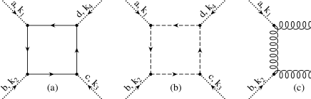
FIG. 1.: Contributions to $\Gamma^{abcd}_{0000}$: (a) fermions, (b) ghosts and (c), (d), (e) gluons.

A The fermion contribution

Consider first the contribution from the $N_{\!f}$ massless quarks, with the particular ordering of momenta shown in Fig. 1(a). Using the conservation of momentum, $k_{4}=-(k_{1}+k_{2}+k_{3})$, with $k_{i}=\vec{k}_{i}$, we find

$$\left.\Gamma^{abcd}_{0000}\right|_{(a)_{1}}= \left(\frac{3ig^{4}N_{\!f}}{4\pi^{5/2}}\right){\rm Tr}_{c}(T^{a}T^{b}T^{c}T^{d})\int_{0}^{1}\!\!dy_{1}\!\int_{0}^{1-y_{1}}\!\!\!dy_{2}\!\int_{0}^{1-y_{1}-y_{2}}\!\!\!\!dy_{3}\!\int_{\epsilon-i\infty}^{\epsilon+i\infty}\!\!\frac{dz}{2\pi i}(1-2^{1-z})\Gamma(z)\xi(z)\cos[\pi z/2]\beta^{-z}\times$$ (6)

$$\left[f_{1}^{-z/2}\Gamma(z/2)\left\{\frac{5}{2}\Gamma((1\!-\!z)/2)-6\Gamma((3\!-\!z)/2)+\frac{2}{3}\Gamma((5\!-\!z)/2)\right\}+f_{1}^{-(2+z)/2}\Gamma((2\!+\!z)/2)\times\right.$$

$$\left.\left\{f_{3}\Gamma((1\!-\!z)/2)-\frac{2}{3}f_{2}\Gamma((3\!-\!z)/2)\right\}+\frac{2}{3}f_{4}f_{1}^{-(4+z)/2}\Gamma((1\!-\!z)/2)\Gamma((4\!+\!z)/2)\right]\ ,$$

where $\xi(z)$ is the Riemann Zeta-function and $f_{i}=f_{i}(y_{1},y_{2},y_{3},\vec{k}_{1},\ldots,\vec{k}_{3})$, given explicitly in the appendix, are functions of the Feynman parameters $y_{k}$ and the external momenta $\vec{k}_{j}$. In the high temperature limit, where $|\vec{k}_{i}|\ll T$, we can use the residue theorem to evaluate the $z$-integral by closing the contour on the left side in the complex $z$-plane. Although there is seemingly a logarithmic dependence on $T$ from a double-pole at $z=0$, coming from the product $\Gamma(z)\Gamma(z/2)$, the coefficient is actually proportional to $[(5/2)\Gamma(1/2)-6\Gamma(3/2)+(2/3)\Gamma(5/2)]=0$. This is in accordance with the fact that the fermion loop does not have any logarithmic enhancements [23].

For the term of order $\beta^{2}$ we get, from the poles at $z=-2$,

$$\left.\Gamma^{abcd}_{0000}\right|_{(a)_{1}}=\left(\frac{-7ig^{4}N_{\!f}\xi(3)\beta^{2}}{96\pi^{4}}\right){\rm Tr}_{c}(T^{a}T^{b}T^{c}T^{d})\left(k_{1}^{2}+2k_{2}^{2}+k_{3}^{2}+2k_{1}k_{2}+2k_{2}k_{3}\right)\ .$$ (7)

When the additional five permutations are added and the resulting four-point function inserted into Eq. (3), the contribution to the effective action from the quark loop becomes,

$$\left.\Gamma_{\!E}\right|_{(a)}(A_{0})=\frac{7g^{4}N_{\!f}\xi(3)\beta^{2}}{2304\pi^{4}}\int_{0}^{\beta}\!d\tau\!\int\!d^{3}x\!\left[2A_{0}^{a}A_{0}^{a}(\partial_{i}A_{0}^{b})^{2}+(\partial_{i}(A_{0}^{a}A_{0}^{a}))^{2}-2f^{acm}f^{bdm}(\partial_{i}A_{0}^{a})\!\cdot\!(\partial_{i}A_{0}^{b})A_{0}^{c}A_{0}^{d}\right]\ ,$$ (8)

after a partial integration.

In the QED case we have $N_{\!f}{\rm Tr}_{c}(T^{a}T^{b}T^{c}T^{d})\rightarrow 1$, and then our result for the two-derivative part of the QED effective action agrees with the earlier calculation in [19].

B The pure Yang-Mills contribution

We now turn to the pure Yang-Mills contribution, i.e. the diagrams (b)-(e) in Fig. 1. To evaluate the finite $T$ part of these diagrams we will use the gauge condition $\partial\!\cdot\!A^{a}=0$, and work in Feynman gauge. As in the fermion case, the functions $g_{i}=g_{i}(y_{1},\ldots,\vec{k}_{1},\ldots,\vec{k}_{3})$ below are all functions of the relevant Feynman parameters and the external momenta. Their explicit forms can also be found in the appendix. Proceeding in a way similar to the previous section, we have for the ghost loop depicted in Fig. 1(b),

$$\left.\Gamma^{abcd}_{0000}\right|_{(b)_{1}}= \frac{-ig^{4}}{8\pi^{5/2}}(f\!f\!f\!f)\!\int_{0}^{1}\!\!dy_{1}\!\int_{0}^{1-y_{1}}\!\!\!dy_{2}\!\int_{0}^{1-y_{1}-y_{2}}\!\!\!\!dy_{3}\!\int_{1+\epsilon-i\infty}^{1+\epsilon+i\infty}\!\!\frac{dz}{2\pi i}\Gamma(z)\xi(z)\cos[\pi z/2](\beta^{2}g_{1})^{-z/2}\Gamma((5\!-\!z)/2)\Gamma(z/2),$$ (9)

where the color structure is $f\!f\!f\!f=f^{fae}\!f^{ebg}\!f^{gch}\!f^{hdf}=\delta_{ab}\delta_{cd}\!+\!\delta_{ad}\delta_{bc}\!+\!N(d_{abm}d_{cdm}\!-\!d_{acm}d_{bdm}\!+\!d_{adm}d_{bcm})/4$, with $N=3$ and $d_{ijk}$ the completely symmetric structure constant.

For the graph in (c) we find,

$$\left.\Gamma^{abcd}_{0000}\right|_{(c)_{1}}= \left(\frac{3ig^{4}}{16\pi^{5/2}}\right)(f\!f\!f\!f)\int_{0}^{1}\!\!dy_{1}\!\int_{0}^{1-y_{1}}\!\!\!dy_{2}\!\int_{0}^{1-y_{1}-y_{2}}\!\!\!\!dy_{3}\!\int_{1+\epsilon-i\infty}^{1+\epsilon+i\infty}\!\!\frac{dz}{2\pi i}\Gamma(z)\xi(z)\cos[\pi z/2]\beta^{-z}\times$$ (12)

$$\left[g_{2}^{-z/2}\Gamma(z/2)\left\{5\Gamma((1\!-\!z)/2)+16\Gamma((3\!-\!z)/2)+32\Gamma((5\!-\!z)/2)\right\}-g_{2}^{-(2+z)/2}\Gamma((2\!+\!z)/2)\times\right.$$

$$\left.\left\{g_{4}\Gamma((1\!-\!z)/2)-\frac{16}{3}g_{3}\Gamma((3\!-\!z)/2)\right\}-\frac{2}{3}g_{5}g_{2}^{-(4+z)/2}\Gamma((1\!-\!z)/2)\Gamma((4\!+\!z)/2)\right]\ ,$$

where the color structure is as for the ghost loop.

For the triangle diagram (d) we get,

$$\left.\Gamma^{abcd}_{0000}\right|_{(d)_{1}}= \left(\frac{-ig^{4}}{8\pi^{5/2}}\right)(f\!f\!)(f\!f\!+\!f\!f)\int_{0}^{1}\!\!dy_{1}\!\int_{0}^{1-y_{1}}\!\!\!dy_{2}\!\int_{1+\epsilon-i\infty}^{1+\epsilon+i\infty}\!\!\frac{dz}{2\pi i}\Gamma(z)\xi(z)\cos[\pi z/2](\beta^{2}g_{6})^{-z/2}\times$$ (14)

$$\left[g_{6}^{-1}(g_{6}-3g_{7})\Gamma((1\!-\!z)/2)\Gamma((2\!+\!z)/2)-15\Gamma((3\!-\!z)/2)\Gamma(z/2)\right]\ ,$$

where $(f\!f\!)(f\!f\!+\!f\!f)=f^{hfc}\!f^{gdf}(f^{age}\!f^{bhe}\!+\!f^{ahm}\!f^{bgm})=-2\delta_{ab}\delta_{cd}\!-\!\delta_{ac}\delta_{bd}\!-\!\delta_{ad}\delta_{bc}\!-\!Nd_{abm}d_{cdm}/2$.

Finally, we find for graph (e),

$$\left.\Gamma^{abcd}_{0000}\right|_{(e)_{1}}= \left(\frac{3ig^{4}}{16\pi^{5/2}}\right)(f\!f\!+\!f\!f)(f\!f\!+\!f\!f)\int_{0}^{1}\!\!dy_{1}\!\int_{1+\epsilon-i\infty}^{1+\epsilon+i\infty}\!\!\frac{dz}{2\pi i}\Gamma(z)\xi(z)\cos[\pi z/2](\beta^{2}g_{8})^{-z/2}\Gamma((1\!-\!z)/2)\Gamma(z/2)\ ,$$ (15)

with $(f\!f\!+\!f\!f)(f\!f\!+\!f\!f)=(f^{age}\!f^{bhe}\!+\!f^{ahe}\!f^{bge})(f^{cgf}\!f^{dhf}\!+\!f^{chf}\!f^{dgf})=4\delta_{ab}\delta_{cd}\!+\!2\delta_{ac}\delta_{bd}\!+\!2\delta_{ad}\delta_{bc}\!+\!Nd_{abm}d_{cdm}$.

Contrary to the fermion case, at order $O(\beta^{0})$ each diagram contains a logarithmic dependence on $T$ and the external momenta $\vec{k}_{j}$. In addition, the $T=0$ part depends logarithmically on $\vec{k}_{j}$ and an ultraviolet cut-off $\Lambda$, that has to be introduced to regularize the loop-momentum integral. The logarithmic dependence on $\vec{k}_{j}$ cancels out between the $T=0$ and $T>0$ parts for each permutation of each individual diagram, whereas the terms containing $\log T$ ($\log\Lambda$) only cancel out in the total $T>0$ ($T=0$) result, i.e. when all the different diagrams are added together. This was basically noted already in [18], and we have checked that it holds true in our calculations as well. There is also a linear divergence when $\beta k\rightarrow 0$, at order $O(1/\beta)$, in all of the Eqs. (9)-(15). This divergence originates from static propagators running in the loop, i.e. the propagators with a vanishing Matsubara frequency, $\omega_{n}=0$. If only the non-static modes are integrated out, the static terms should be subtracted and our remaining result is then finite in the limit $\beta k\rightarrow 0$, as it should [18]. We emphasize that the $\omega_{n}=0$ modes do not influence the two-derivative term.

Taking into account all the permutations of Eqs. (9)-(15) and adding the different contributions, we find for the $O(\beta^{2})$ term,

$$\left.\Gamma_{\!E}\right|_{(b)-(e)}(A_{0})=-\frac{g^{4}\xi(3)\beta^{2}}{256\pi^{4}}\int_{0}^{\beta}\!d\tau\!\int\!d^{3}x\!\left[2A_{0}^{a}A_{0}^{a}(\partial_{i}A_{0}^{b})^{2}+(\partial_{i}(A_{0}^{a}A_{0}^{a}))^{2}+\frac{11}{6}f^{acm}f^{bdm}(\partial_{i}A_{0}^{a})\!\cdot\!(\partial_{i}A_{0}^{b})A_{0}^{c}A_{0}^{d}\right]\ ,$$ (16)

where we have performed an integration by parts. This result for the pure Yang-Mills contribution disagrees slightly with the previous finding from the background field method in [20], in that the first two term in Eq. (16) are a factor $(2/11)$ smaller, and the last a factor $(-1/2)$.

C The total contribution

By combining the results in Eqs. (8) and (16), the complete contribution to the effective action becomes,

$$\Gamma_{\!E}^{(4)}(A_{0})= \left.\Gamma_{\!E}\right|_{(a)}(A_{0})+\left.\Gamma_{\!E}\right|_{(b)-(e)}(A_{0})=\frac{g^{4}\xi(3)\beta^{2}}{256\pi^{4}}\left(\frac{7N_{\!f}}{9}-1\right)\int_{0}^{\beta}\!d\tau\!\int\!d^{3}x\!\left[2A_{0}^{a}A_{0}^{a}(\partial_{i}A_{0}^{b})^{2}+(\partial_{i}(A_{0}^{a}A_{0}^{a}))^{2}\right]-$$ (18)

$$\frac{11g^{4}\xi(3)\beta^{2}}{1536\pi^{4}}\left(\frac{28N_{\!f}}{33}+1\right)\int_{0}^{\beta}\!d\tau\!\int\!d^{3}x\!\left[f^{acm}f^{bdm}(\partial_{i}A_{0}^{a})\!\cdot\!(\partial_{i}A_{0}^{b})A_{0}^{c}A_{0}^{d}\right]\ .$$

In the dimensionally reduced theory of QCD [18, 19], Eq. (18) provides the leading derivative interactions between the $A_{0}$-fields. How large the calculated derivative term is, compared to both the ones already present in Eq. (2) as well as the omitted higher dimension operators, depends on the scales of interest. For instance, at the soft scale where $\partial_{i}\sim gT$ and $A_{0}\sim T$, we have $g^{4}\beta^{2}\partial^{2}A_{0}^{4}\sim g^{6}T^{4}$, a factor $g^{2}$ higher than the term $g^{4}A_{0}^{4}$.

In general, this effective theory is interesting on length scales $|\vec{x}|\ll\beta$ in the high temperature regime, especially when combined with nonperturbative lattice methods [24]. It is for example possible to study the non-perturbative Debye mass [25], and the 3d effective theory is also useful for calculations of the pressure in the quark-gluon phase, both perturbatively [8] and nonperturbatively [26]. Although the derived correction in Eq. (18) presumably gives a minor effect only, it is somewhat interesting to note that the terms are rather sensitive to the number of quark flavors. In Eq. (18), the coefficient of the first term is proportional to $(7N_{\!f}-9)$, which goes from $-1$ to $4/3$ between $N_{\!f}=0$ and $N_{\!f}=3$. Similarly, the second term in Eq. (18) increases by more than 250% in the same range of $N_{\!f}$. This should be contrasted with the constant part of the $A_{0}^{4}$-contribution to Eq. (2), that depends on $N_{\!f}$ as $(9-N_{\!f})$ and therefore only changes by 33% when going from $N_{\!f}=0$ to $N_{\!f}=3$. Due to this strong behavior of the number of quark flavors, it is not inconceivable that the derivative interactions will make a small but noticeable difference between e.g. the pure glue theory and the three-flavor case.

III Derivative terms in the Wilson Line model

The QCD dimensionally reduced theory describes accurately static phenomena at very high $T$, but the approximations break down around a few times $T_{c}$ [24]. In addition, one is by construction omitting all dynamical information.

To understand the features around $T_{c}$ a Ginzburg-Landau type of effective theory was proposed in [12]. In this model, the potential is written in terms of $l$,

$$V(l)=a_{1}T^{4}\left[-a_{2}|l|^{2}-a_{3}\left(l^{3}+{\rm c.c.}\right)+|l|^{4}\right]\ .$$ (19)

The constants $a_{i}$ are then used to fit the pressure above $T_{c}$, with $a_{2}$ a function of temperature so that the global minimum of the potential is at $l\neq 0$ ($l=0$) above (below) $T_{c}$ [16]. One of the important aspects of the potential in Eq. (19) is the extremely rapid change around $T_{c}$, due to a very sensitive dependence of $a_{2}$ on $T/T_{c}$ [16]. In a dynamical scenario one can therefore assume an instantaneous quench, where the value of $l$ suddenly no longer corresponds to the correct minimum. The $l$-field then rolls down the potential, and by coupling the $l$-field to a linear sigma model the potential energy is converted into pions [16, 17]. Even though the model is of phenomenological origin, it thus makes predictions that can be compared to experimental results.

After the quench, the evolution of the Euler-Lagrange equations from the initial conditions requires, apart from the potential and the coupling to the chiral field, also a kinetic term for $l$ [16, 17]. Although the time dependence is beyond the calculation presented in this paper, we can provide the first perturbative QCD-correction to the spatial derivatives. The leading coefficient is the classical contribution to the derivative term, and comes from the kinetic term of $A_{0}(\vec{x})$ in Eq. (2), as can be seen from the following argument [27]: decomposing the Wilson Line in Eq. (1) into an octet $\tilde{{\bf L}}$ and the singlet $l$,

$${\bf L}=\tilde{{\bf L}}+{\bf 1}\frac{1}{N}{\rm Tr}\,{\bf L}=\tilde{{\bf L}}+{\bf 1}l\ ,$$ (20)

where $\tilde{{\bf L}}$ is traceless and $N=3$, we have

$${\rm Tr}|\partial_{i}{\bf L}|^{2}={\rm Tr}|\partial_{i}\tilde{{\bf L}}|^{2}+3|\partial_{i}l|^{2}\ .$$ (21)

On the other hand, by a direct calculation in the static limit,

$${\rm Tr}|\partial_{i}{\bf L}|^{2}=g^{2}\beta^{2}(\partial_{i}A_{0}^{a})^{2}+{\rm Tr}\,\left\{{\rm commutator\,terms}\right\}\ .$$ (22)

When the commutator terms in Eq. (22) are rewritten in terms of ${\bf L}$ they can only involve the adjoint field, or products of $l$ and $\tilde{{\bf L}}$, since $l$ (times the identity matrix) by itself commutes with all SU(3) matrices. Thus, by combining Eqs. (21) and (22), we have,

$$(1/2)(\partial_{i}A_{0})^{2}=\frac{T^{2}}{2g^{2}}\left[{\rm Tr}|\partial_{i}\tilde{{\bf L}}|^{2}+3|\partial_{i}l|^{2}\right]+f(\tilde{{\bf L}})\ ,$$ (23)

where $f(\tilde{{\bf L}})$ corresponds to the commutator terms, rewritten as a function of $\tilde{{\bf L}}$. At $T_{c}$, $g\simeq 2.5$ so that the leading coefficient for the kinetic term of $l$ is $3/2g^{2}\simeq 0.3$, which is reasonably close to the canonical value $1/2$. Given the unknown function $f(\tilde{{\bf L}})$ it is not clear whether the kinetic term for the adjoint field actually is unique. However, $\tilde{{\bf L}}$ does not play any important role around $T_{c}$, and can therefore be neglected on physical grounds [12].

The procedure to obtain the kinetic term for $l$ is thus to match terms in the effective theory $\Gamma(A_{0})$ to a corresponding $|\partial_{i}l|^{2}$ piece in $\Gamma(l)$. This means that the classical coefficient for $|\partial_{i}l|^{2}$ will change when radiative corrections are taken into account in $\Gamma(A_{0})$. To lowest order, the kinetic term for $A_{0}$ can receive corrections from the polarization tensor [18, 19], that would affect the $|\partial_{i}l|^{2}$ term via Eq. (23). However, with the optimal choice for the counterterms [19] there is in fact no $O(g^{2})$-contribution, so the renormalized kinetic term in $\Gamma(A_{0})$ remains $(1/2)(\partial_{i}A_{0})^{2}$.

Even though the kinetic term for $A_{0}$ is unchanged at one-loop, this does not mean that $|\partial_{i}l|^{2}$ is so. Since $l=(1/3){\rm Tr}\,{\bf L}$, the $|\partial_{i}l|^{2}$-term contains at least four powers of $A_{0}$ when ${\bf L}$ is expanded in powers of $A_{0}$. The two-derivative term in $\Gamma(l)$ can therefore receive a perturbative correction from the four-point function in Eq. (3). Indeed, by using the relations

$$A_{0}^{a}A_{0}^{a}(\partial_{i}A_{0}^{b})^{2}= -\frac{12}{g^{4}\beta^{4}}\left[|l|^{2}-1\right]\left({\rm Tr}|\partial_{i}\tilde{{\bf L}}|^{2}+3|\partial_{i}l|^{2}\right)+O(A_{0}^{6})\ ,$$ (24)

$$(\partial_{i}(A_{0}^{a}A_{0}^{a}))^{2}= \frac{144}{g^{4}\beta^{4}}|\partial_{i}l|^{2}+O(A_{0}^{6})$$ (25)

$$f^{acm}f^{bdm}(\partial_{i}A_{0}^{a})\!\cdot\!(\partial_{i}A_{0}^{b})A_{0}^{c}A_{0}^{d}= 2{\rm Tr}|[\partial_{i}\tilde{{\bf L}},\ \tilde{{\bf L}}]|^{2}+O(A_{0}^{6})\ ,$$ (26)

we can rewrite Eq. (18) as

$$\Gamma_{\!E}= \int_{0}^{\beta}\!d\tau\!\int\!d^{3}x\!\left\{\frac{\xi(3)T^{2}}{16\pi^{4}}\left(\frac{7N_{\!f}}{9}-1\right)\left[\frac{3}{2}(1-|l|^{2}){\rm Tr}|\partial_{i}\tilde{{\bf L}}|^{2}+\frac{27}{2}|\partial_{i}l|^{2}-\frac{9}{2}|l|^{2}|\partial_{i}l|^{2}\right]\right.-$$ (28)

$$\left.\frac{11\xi(3)T^{2}}{768\pi^{4}}\left(\frac{28N_{\!f}}{33}+1\right){\rm Tr}|[\partial_{i}\tilde{{\bf L}},\ \tilde{{\bf L}}]|^{2}\right\}\ .$$

From the calculation of the four-point function we thus find the leading perturbative correction to the kinetic term of $l$. Including the contribution from Eq. (28), the kinetic term now becomes

$$\frac{3T^{2}}{2g^{2}}|\partial_{i}l|^{2}\rightarrow\frac{3T^{2}}{2g^{2}}\left[1+\frac{g^{2}\xi(3)}{16\pi^{4}}(7N_{\!f}-9)\right]|\partial_{i}l|^{2}=\frac{3T^{2}}{2g^{2}}\left[1+c_{{\rm corr}}\right]|\partial_{i}l|^{2}\ .$$ (29)

Since $l$ is dimensionless, the correct dimension of the operator has to be supplied by some other scales. In the perturbative calculation the only scale is $T$, and hence the one-loop induced coefficient has the same $T$-dependence as the leading term in Eq. (23). However, the perturbative correction does not depend on the QCD coupling constant and is therefore just a fixed number at this order. For example, for three flavors the coefficient is $\simeq 1.4\times 10^{-2}T^{2}$. Compared to the classical contribution $(3/2g^{2})T^{2}$, the fraction of the one-loop correction is only $0.01g^{2}$. Even at $T_{c}$, this is merely of the order of 5%, and at higher $T$ even less due to the logarithmic decrease of $g$.

Having derived the first correction to the kinetic term for $l$ from perturbation theory, let us now discuss to what extent, and in what temperature range, the terms in Eq. (28) can be trusted. First of all, it should be noted that the form of the effective action in Eq. (28) is not completely unique. The reason is that by a partial integration, and discarding any surface terms, we can always trade factors of $[A_{0}^{a}A_{0}^{a}(\partial_{i}A_{0}^{b})^{2}]$ and $(\partial_{i}(A_{0}^{a}A_{0}^{a}))^{2}$ for a term like $[A_{0}^{a}A_{0}^{a}A_{0}^{b}(\partial_{i}^{2}\!A_{0}^{b})]$, but this equality does not hold at the level of $l$. In fact, if a term $[A_{0}^{a}A_{0}^{a}A_{0}^{b}(\partial_{i}^{2}\!A_{0}^{b})]$ is kept in the action, not only do the coefficients in Eq. (28) change, but there are also additional nonequivalent terms of the form $(\partial_{i}|l|^{2})^{2}$ and $|l|^{2}[\partial_{i}^{2}(l+l^{\ast})]$. Nevertheless, the action in Eq. (28) is of course unique to order $O(A_{0}^{4})$. Since higher order operators in the dimensionally reduced theory are further suppressed at high $T$, the predictions in Eq. (28) should at the very least be reliable down to $T\geq 2T_{c}-3T_{c}$, i.e. when the effective 3d theory itself is applicable.

When $T\rightarrow T_{c}$, the question is admittedly more subtle, as higher loop effects, higher dimensional operators and possibly nonperturbative effects become important. However, Eq. (28) does not have to break down completely when the 3d theory does so. The 3d theory becomes invalid because the procedure of integrating out the non-static modes is unreliable when $g^{2}(T)\,T\simeq\pi T$ [24]. In contrast, $\Gamma(l)$ is by construction valid near $T_{c}$, so the question is rather how much the coefficient for the spatial derivative term changes.

Considering first the operators of higher dimensionality, it is certainly possible to imagine that their bulk part follows from an expansion of Eq. (28). The additional contributions that do not originate from these sources, e.g. terms like $T^{2}(|l|^{2}-1)^{n}|\partial_{i}l|^{2}$, that are at least of order $A_{0}^{(2n+2)}$ (with $n\geq 2$), would then be suppressed. Not because they are unimportant a priori, but because their numerical coefficients are small. There are also higher derivative terms not accounted for in Eq. (28), like $(|l|^{2}-1)(\partial_{i}^{2}|l|^{2})^{2}$, but they do not affect the kinetic term. To $O(A_{0}^{4})$, they are in fact straightforward to obtain from Eq. (6) and Eqs. (9)-(15).

When it comes to higher loop and nonperturbative effects, they will naturally induce a $T$-dependence in the radiative corrections to the kinetic term. Thus, $(3T^{2}/2g^{2})(1+c_{\rm corr})|\partial_{i}l|^{2}\rightarrow(3T^{2}/2g^{2})(1+c_{\rm corr}(T/T_{c},T/\Lambda))|\partial_{i}l|^{2}$, which follows partly from the running of the QCD coupling constant in the higher loop effects. How much this will affect the kinetic term is difficult to estimate, but the small correction from the four-point function may indicate that the perturbative QCD-contributions are not too important for constructing $\Gamma(l)$.

IV Summary and Conclusions

In this paper we calculated the leading momentum dependence of the four-point function in QCD with $N_{\!f}$ massless flavors, and related this contribution to terms in both the effective action $\Gamma(A_{0})$ and $\Gamma(l)$.

As for the derivative terms in $\Gamma(A_{0})$, they will only have a minor influence when $T\gg T_{c}$. As the temperature decreases and approaches $T_{c}$ the 3d theory becomes less reliable, but there could very well be a temperature region where the effective theory is still valid and the derivative interactions nonnegligible. Since the contribution has a rather strong dependence on $N_{\!f}$, a difference between the pure glue theory and e.g. $N_{\!f}=3$ QCD could perhaps be noticed.

From the four-point function, we also found the lowest one-loop QCD correction to the spatial derivative term in the effective theory $\Gamma(l)$. The coefficient is independent of $g$ and much smaller than the classical term, the ratio between the two being of the order of $10^{-2}$ at $T_{c}$. This derivation assumes that the strange quark mass $m_{s}$ can be neglected even at $T_{c}$, which of course is an oversimplification, given that $m_{s}\sim T_{c}$. Nevertheless, the influence of $m_{s}$ is not likely to change the fact that the correction is small even at $T_{c}$.

At one-loop, there is an infinite number of terms that contribute to the coefficient of $|\partial_{i}l|^{2}$, to the same order in $g$ and $T$, as the four-point function. This follows from the fact the induced two-derivative interactions, with $n$ external fields $A_{0}$, is of the functional form $g^{n}\partial^{2}A_{0}^{n}/T^{(n-2)}$, which corresponds to an expansion of $l$ to at most order $(n-2)$ in the term $T^{2}|\partial_{i}l|^{2}$. Some of these higher-dimensional contributions, maybe even the major parts, are already accounted for by rewriting the four-point function in $\Gamma(A_{0})$ in terms of $l$, as in Eq. (28). In any case, since the four-point contribution is very small, it is reasonable to assume that the higher $n$-point functions give even smaller corrections. In that case, Eq. (28) should give the correct order of magnitude for the total one-loop correction.

As mentioned earlier, there are also higher loop effects that contribute to the kinetic term in $\Gamma(l)$. For example, taking into account the two-loop correction to the diagrams in Fig. 1 gives $c_{{\rm corr}}\rightarrow c_{{\rm corr}}[1+ag^{2}]$. To understand the reliability of the canonical term it is then crucial to know the magnitude of $a$. Surprisingly, studies of higher loop effects in the 3d effective theory $\Gamma(A_{0})$ indicate that they only give corrections of the order of 30% at $T_{c}$ [24]. If these conjectures can be taken over to the Wilson Line model, one could in fact expect the derivative term $(1/2)|\partial_{i}l|^{2}$ to change by perhaps at most a factor two, with all QCD-corrections taken into account. Of course, this has to be regarded as a highly speculative suggestion at the present stage.

To complete the dynamical scenario one also needs the time dependence of $l$. Unfortunately, it is yet unclear how $l$ generalizes to a real time formulation [12]. Assuming that the form of the spatial derivatives can be extended to a Lorentz invariant form, the predictions for pion production and the evolution of $|l|$ will remain almost unchanged [16, 17]. In particular, if the Lorentz invariant kinetic term does not change by more than a factor of two, it can easily be compensated by a difference in e.g. the expansion rate of the plasma.

Finally, to obtain a decisive estimate of the QCD-effects in $\Gamma(l)$, one has to establish either a unique mapping from $\Gamma(A_{0})$ to $\Gamma(l)$, or find a way to determine $\Gamma(l)$ directly, perhaps numerically. Hopefully, the calculations presented in this paper can serve as a first step in that direction.

Acknowledgments

The author thanks R. D. Pisarski for discussions that initialized this project, and for reading the manuscript. D. Bödeker, A. Dumitru and R. D. Pisarski are greatfully acknowledged for useful and interesting discussions during the investigations, and K. Kajantie and M. Laine for useful comments on an early version of the manuscript. This work was supported by The Swedish Foundation for International Cooperation in Research and Higher Education (STINT) under contract 99/665, and in part by DOE grant DE-AC02-98CH10886.

A Evaluation of the Feynman diagrams

In this appendix we outline our method for calculating the Feynman diagrams shown in Fig. 1. We first follow the Feynman rules given in [28] for Minkowski space-time. After all contractions and traces over spinor indices have been performed, we continue to a Euclidean space compact in the imaginary time direction:

$$p_{0}\rightarrow i\omega_{n}\ ,\ \ \ \ \int\frac{dp_{0}}{2\pi}\rightarrow iT\sum_{n}\ ,$$ (A1)

where $\omega_{n}$ is the Matsubara frequency, $\omega_{n}=(2n+1)\pi T$ ($\omega_{n}=2\pi T$) for fermions (bosons).

Next, we use a Feynman parametrization to combine the denominators in the loop integral, and extract the $T>0$ part from the following relations [22]:

$$\left.T\sum_{n}f(p_{0}=i\omega_{n})\right|_{T>0}=\left\{\matrix{&\int_{\delta-i\infty}^{\delta+i\infty}\frac{dp_{0}}{2\pi i}\,n_{B}\,[f(p_{0})+f(-p_{0})]\ \ {\rm(bosons)}\cr&\mbox{}\cr&\int_{\delta-i\infty}^{\delta+i\infty}\frac{dp_{0}}{2\pi i}\,n_{F}\,[f(p_{0})+f(-p_{0})]\ \ {\rm(fermions)}}\right.\ .$$ (A2)

where $n_{B}=[\exp(\beta p_{0})-1]^{-1}$, $n_{F}=[\exp(\beta p_{0})+1]^{-1}$ and $\delta\rightarrow 0^{+}$. The ghosts follow Bose statistics, despite their anticommuting properties.

By shifting the vector momentum in the loop, $\vec{p}$, to $\vec{q}=\vec{p}+h(y_{i},\vec{k}_{i})$, with $h(y_{i},\vec{k}_{i})$ a linear function of the external momenta $\vec{k}_{i}$, we then integrate over $\vec{q}$. Finally, by performing a Mellin transform,

$$\left(e^{x}\pm 1\right)^{-1}=\int_{c_{\pm}-i\infty}^{c_{\pm}+i\infty}\frac{dz}{2\pi i}\Gamma(z)\xi(z)v_{\pm}x^{-z}\ ,$$ (A3)

where $v_{+}=(1-2^{1-z})$, $v_{-}=1$, and with the contour specified by $c_{+}=\epsilon$, $c_{-}=1+\epsilon$ (where $\epsilon\rightarrow 0^{+}$), we can integrate over $p_{0}$ after a change of variables.

To illustrate the above procedure, consider the diagram in Fig. 1(e). Omitting the color factors for simplicity, and using the notation $|\vec{p}|=p$, $|\vec{k}_{1}+\vec{k}_{2}|=|\vec{k}_{12}|=k_{12}$, we have to calculate the following integral:

$$\frac{3g^{4}}{2}\!\int\!\frac{d^{4}p}{(2\pi)^{4}}\,\frac{1}{p_{0}^{2}-p^{2}}\,\frac{1}{p_{0}^{2}-(p+k_{12})^{2}}\stackrel{{\scriptstyle T>0}}{{\rightarrow}}3ig^{4}\!\int_{\delta-i\infty}^{\delta+i\infty}\!\frac{dp_{0}}{2\pi i}n_{B}\!\int_{0}^{1}\!dy_{1}\!\int\!\frac{d^{3}p}{(2\pi)^{3}}\frac{1}{[p^{2}+\{2\vec{p}\cdot\vec{k}_{12}+k_{12}^{2}\}(1\!-\!y_{1})-p_{0}^{2}]^{2}}$$ (A4)

$$\ \ \ \ =\frac{3ig^{4}}{2\pi^{2}}\int_{0}^{1}dy_{1}\int_{\delta-i\infty}^{\delta+i\infty}\frac{dp_{0}}{2\pi i}n_{B}\int_{0}^{\infty}dq\frac{q^{2}}{[q^{2}+g_{8}-p_{0}^{2}]^{2}}\ ,$$ (A5)

where we made the shift $\vec{q}=\vec{p}+(1-y_{1})\vec{k}_{12}$ and defined $g_{8}=y_{1}(1-y_{1})k_{12}^{2}$ in the last integral. After performing the $q$-integral in Eq. (A5), we are left with,

$$\frac{3ig^{4}}{8\pi}\!\int_{0}^{1}\!dy_{1}\int_{\delta-i\infty}^{\delta+i\infty}\frac{dp_{0}}{2\pi i}\left(\frac{1}{e^{\beta p_{0}}\!-\!1}\right)\frac{1}{\sqrt{g_{8}-p_{0}^{2}}}=\frac{3ig^{4}}{8\pi^{2}}\!\int_{0}^{1}\!dy_{1}\int_{1+\epsilon-i\infty}^{1+\epsilon+i\infty}\frac{dz}{2\pi i}\Gamma(z)\xi(z)\cos[\pi z/2]\beta^{-z}\!\int_{0}^{\infty}\!du\frac{u^{-z}}{\sqrt{g_{8}+u^{2}}}$$ (A6)

$$\ \ \ =\frac{3ig^{4}}{16\pi^{5/2}}\int_{0}^{1}dy_{1}\int_{1+\epsilon-i\infty}^{1+\epsilon+i\infty}\frac{dz}{2\pi i}\Gamma(z)\xi(z)\beta^{-z}\cos[\pi z/2]g_{8}^{-z/2}\Gamma((1-z)/2)\Gamma(z/2)\ ,$$ (A7)

which is Eq. (15), except for the color factors.

To check our method we also calculated the $O(\beta^{2}k_{12}^{2})$ contribution to the above diagram in a different way: we first performed the $p_{0}$-integral, by picking up the poles in the complex $p_{0}$-plane, and then did the $p$-integral, without any Feynman parametrization, by expanding the integrand differently in different integration regions. The two results of course agree with each other.

For completeness, we also give the functions $f_{1},\ldots,f_{4}$ in Eq. (6) and $g_{1},\ldots,g_{8}$ in Eqs. (9)-(15). Using the conservation of momentum, and the shorthand notation $\vec{k}_{i}+\vec{k}_{j}+\vec{k}_{l}=k_{ijl}$, their explicit forms are as follows:

$$f_{1}= y_{2}k_{1}^{2}+y_{3}k_{12}^{2}+(1-y_{1}-y_{2}-y_{3})k_{123}^{2}-[y_{2}k_{1}+y_{3}k_{12}+(1-y_{1}-y_{2}-y_{3})k_{123}]^{2}$$ (A8)

$$f_{2}= 3k_{1}^{2}+4k_{1}k_{2}+k_{2}^{2}+2k_{1}k_{3}+k_{2}k_{3}-3(3k_{1}+2k_{2}+k_{3})[y_{2}k_{1}+y_{3}k_{12}+(1-y_{1}-y_{2}-y_{3})k_{123}]+$$ (A10)

$$+6[y_{2}k_{1}+y_{3}k_{12}+(1-y_{1}-y_{2}-y_{3})k_{123}]^{2}$$

$$f_{3}= (1/3)\left\{5k_{1}^{2}y_{1}(2y_{1}-1)+k_{2}^{2}[3+10y_{1}^{2}-10y_{2}+10y_{2}^{2}+10y_{1}(2y_{2}-1)]++5k_{3}^{2}[1+2y_{1}^{2}+2y_{2}^{2}-3y_{3}+2y_{3}^{2}+\right.$$ (A13)

$$+y_{2}(4y_{3}-3)+y_{1}(4y_{2}+4y_{3}-3)]+k_{2}k_{3}[8+20y_{1}^{2}+20y_{2}^{2}-10y_{3}+5y_{2}(4y_{3}-5)+5y_{1}(8y_{2}+4y_{3}-5)]+$$

$$\left.k_{1}[k_{2}(3+20y_{1}^{2}-5y_{2}+5y_{1}(4y_{2}-3))+k_{3}(2+20y_{1}^{2}-5y_{2}-5y_{3}+20y_{1}(y_{2}+y_{3}-1))]\right\}$$

$$f_{4}= \left\{[(1-y_{2})k_{1}-y_{3}k_{12}-(1-y_{1}-y_{2}-y_{3})k_{123}]\cdot[-y_{2}k_{1}+(1-z)k_{12}-(1-y_{1}-y_{2}-y_{3})k_{123}]\right\}\times$$ (A19)

$$\left\{[-y_{2}k_{1}-y_{3}k_{12}-(1-y_{1}-y_{2}-y_{3})k_{123}]\cdot[-y_{2}k_{1}-y_{3}k_{12}+(y_{1}+y_{2}+y_{3})k_{123}]\right\}-$$

$$-\left\{[-y_{2}k_{1}-y_{3}k_{12}-(1-y_{1}-y_{2}-y_{3})k_{123}]\cdot[-y_{2}k_{1}+(1-z)k_{12}-(1-y_{1}-y_{2}-y_{3})k_{123}]\right\}\times$$

$$\left\{[(1-y_{2})k_{1}-y_{3}k_{12}-(1-y_{1}-y_{2}-y_{3})k_{123}]\cdot[-y_{2}k_{1}-y_{3}k_{12}+(y_{1}+y_{2}+y_{3})k_{123}]\right\}+$$

$$+\left\{[-y_{2}k_{1}-y_{3}k_{12}-(1-y_{1}-y_{2}-y_{3})k_{123}]\cdot[(1-y_{2})k_{1}-y_{3}k_{12}-(1-y_{1}-y_{2}-y_{3})k_{123}]\right\}\times$$

$$\left\{[-y_{2}k_{1}+(1-z)k_{12}-(1-y_{1}-y_{2}-y_{3})k_{123}]\cdot[-y_{2}k_{1}-y_{3}k_{12}+(y_{1}+y_{2}+y_{3})k_{123}]\right\}$$

$$g_{1}= f_{1}$$ (A20)

$$g_{2}= f_{1}$$ (A21)

$$g_{3}= 3k_{1}^{2}+2k_{2}^{2}+2k_{3}^{2}+3k_{1}k_{2}+3k_{1}k_{3}+2k_{2}k_{3}+2[(1-y_{1})k_{1}+(1-y_{1}-y_{2})k_{2}+(1-y_{1}-y_{2}-y_{3})k_{3}]^{2}-$$ (A23)

$$-(3k_{1}+2k_{2}+k_{3})[(1-y_{1})k_{1}+(1-y_{1}-y_{2})k_{2}+(1-y_{1}-y_{2}-y_{3})k_{3}]$$

$$g_{4}= (1/3)\left\{k_{1}^{2}(10y_{1}-20y_{1}^{2}-7)-2k_{2}^{2}[10y_{1}^{2}-10y_{2}+10y_{2}^{2}+10y_{1}(2y_{2}-1)-3]-\right.$$ (A27)

$$-k_{3}^{2}[17+20y_{1}^{2}+20y_{2}^{2}-30y_{3}+20y_{3}^{2}+10y_{2}(4y_{3}-3)+10y_{1}(4y_{2}+4y_{3}-3)]-$$

$$-2k_{2}k_{3}[2+20y_{1}^{2}+20y_{2}^{2}-10y_{3}+5y_{2}(4y_{3}-5)+5y_{1}(8y_{2}+4y_{3}-5)]-$$

$$\left.-2k_{1}[k_{2}(20y_{1}^{2}-5y_{2}+5y_{1}(4y_{2}-3)-3)+5k_{3}(3+4y_{1}^{2}-y_{2}-y_{3}+4y_{1}(y_{2}+y_{3}-1))]\right\}$$

$$g_{5}= \left\{[y_{1}k_{1}+(1+y_{1}+y_{2})k_{2}-(1-y_{1}-y_{2}-y_{3})k_{3}]\cdot[(2-y_{1})k_{1}+(1-y_{1}-y_{2})k_{2}+(1-y_{1}-y_{2}-y_{3})k_{3}]\right\}\times$$ (A31)

$$\left\{[-y_{1}k_{1}-(y_{1}+y_{2})k_{2}+(2-y_{1}-y_{2}-y_{3})k_{3}]\cdot[(2-y_{1})k_{1}+(2-y_{1}-y_{2})k_{2}+(2-y_{1}-y_{2}-y_{3})k_{3}]\right\}+$$

$$\left\{[(1+y_{1})k_{1}-(1-y_{1}-y_{2})k_{2}-(1-y_{1}-y_{2}-y_{3})k_{3}]\cdot[(1+y_{1})k_{1}+(1+y_{1}+y_{2})k_{2}+(1+y_{1}+y_{2}+y_{3})k_{3}]\right\}\times$$

$$\left\{[-y_{1}k_{1}+(2-y_{1}-y_{2})k_{2}+(1-y_{1}-y_{2}-y_{3})k_{3}]\cdot[y_{1}k_{1}+(y_{1}+y_{2})k_{2}+(1+y_{1}+y_{2}+y_{3})k_{3}]\right\}$$

$$g_{6}= y_{1}k_{12}^{2}+y_{2}k_{123}^{2}+(1-y_{1}-y_{2})k_{1234}^{2}-[k_{1}+k_{2}+(1-y_{1})k_{3}+(1-y_{1}-y_{2})k_{4}]^{2}$$ (A32)

$$g_{7}= [(1+y_{1})k_{3}-(1-y_{1}-y_{2})k_{4}][(2-y_{1}-y_{2})k_{4}-y_{1}k_{3}]\ ,$$ (A33)

where, in order to simplify the permutations of the triangle graph, we did not use $k_{4}=-(k_{1}+k_{2}+k_{3})$ in Eqs. (A32) and (A33). Finally,

$$\hskip 2.0ptg_{8}=y_{1}(1-y_{1})k_{12}^{2}\ .$$ (A34)

REFERENCES

• [1] See the homepage for the conference QM2001: http://www.rhic.bnl.gov/qm2001.
• [2] Y. Iwasaki, K. Kanaya, T. Kaneko and T. Yoshié, Phys. Rev. D56, 151 (1997).
• [3] CP-PACS Coll., Phys. Rev. D63, 034502 (2001); F. Karsch, A. Peikert and E. Laermann, hep-lat/0012023.
• [4] S. Digal, E. Laermann and H. Satz, Eur. Phys. J. C18, 583 (2001).
• [5] Y. Iwasaki, K. Kanaya, S. Kaya, S. Sakai and T. Yoshié, Phys. Rev. D54, 7010 (1996); F. R. Brown et al., Phys. Rev. Lett. 65, 2491 (1990).
• [6] F. Karsch, E. Laermann and A. Peikert, Phys. Lett. B478, 447 (2000).
• [7] P. Arnold and C. Zhai, Phys. Rev. D51, 1906 (1995).
• [8] E. Braaten and A. Nieto, Phys. Rev. D53, 3421 (1996).
• [9] J. C. Taylor and S. M. H. Wong, Nucl. Phys. B346, 115 (1990); E. Braaten and R. D. Pisarski, Phys. Rev. D45, R1827 (1992).
• [10] J.P. Blaizot, E. Iancu and A. Rebhan, Phys. Lett. B470, 181 (1999).
• [11] A. Peshier, Phys. Rev. D63, 105004 (2001).
• [12] R. D. Pisarski, Phys. Rev. D62, 111501 (2000).
• [13] A. Polyakov, Phys. Lett. B72, 477 (1977); L. Susskind, Phys. Rev. D20, 2610 (1979); B. Svetitsky and L. Yaffe, Nucl. Phys. B210, 423 (1982).
• [14] F. Karsch and E. Laermann, Phys. Rev. D50, 6954 (1994).
• [15] L. Kofman, A. Linde and A. A. Starobinsky, Phys. Rev. Lett. 73, 3195 (1994).
• [16] A. Dumitru and R. D. Pisarski, Phys. Lett. B504, 282 (2001); hep-ph/0102020.
• [17] O. Scavenius, A. Dumitru and A. D. Jackson, hep-ph/0103219.
• [18] S. Nadkarni, Phys. Rev. D27, 917 (1983); Phys. Rev. D38, 3287 (1988).
• [19] N. P. Landsman, Nucl. Phys. B322, 498 (1989).
• [20] S. Chapman, Phys. Rev. D50, 5308 (1994).
• [21] T. Appelquist and R. D. Pisarski, Phys. Rev. D23, 2305 (1981).
• [22] J. I. Kapusta, Finite Temperature Field Theory (Cambridge University Press, Cambridge, England, 1989); M. Le Bellac, Thermal Field Theory (Cambridge University Press, Cambridge, England, 1996).
• [23] F. T. Brandt, J. Frenkel and J. C. Taylor, Phys. Rev. D50, 4110 (1994); R. Venugopalan and J. Wirstam, Phys. Rev. D63, 125022 (2001).
• [24] K. Kajantie, M. Laine, K. Rummukainen and M. Shaposhnikov, Nucl. Phys. B503, 357 (1997).
• [25] K. Kajantie, M. Laine, J. Peisa, A. Rajantie, K. Rummukainen and M. Shaposhnikov, Phys. Rev. Lett. 79, 3130 (1997).
• [26] K. Kajantie, M. Laine, K. Rummukainen and Y. Schröder, Phys. Rev. Lett. 86, 10 (2001).
• [27] R. D. Pisarski, private communications.
• [28] M. E. Peskin and D. V. Schroeder, An Introduction to Quantum Field Theory (Addison-Wesley, Reading, USA, 1995).