Neutrino Oscillations with Two $\Delta m^{2}$ Scales

Irina Mocioiu and Robert Shrock

C.N. Yang Institute for Theoretical Physics

State University of New York

Stony Brook, NY 11794-3840

An approximation that is often used in fits to reactor and atmospheric neutrino data and in some studies of future neutrino oscillation experiments is to assume one dominant scale, $\Delta m^{2}$, of neutrino mass squared differences, in particular, $\Delta m^{2}_{atm}\sim 3\times 10^{-3}$ eV². Here we investigate the corrections to this approximation arising from the quantity $\Delta m^{2}_{sol}$ relevant for solar neutrino oscillations, assuming the large mixing angle solution. We show that for values of $\sin^{2}(2\theta_{13})\sim 10^{-2}$ (in the range of interest for long-baseline neutrino oscillation experiments with either intense conventional neutrino beams such as JHF-SuperK or a possible future neutrino factory) and for $\Delta m^{2}_{sol}\sim 10^{-4}$ eV², the contributions to $\nu_{\mu}\to\nu_{e}$ oscillations from both CP-conserving and CP-violating terms involving $\sin^{2}(\Delta m^{2}_{sol}L/(4E))$ can be comparable to the terms involving $\sin^{2}(\Delta m^{2}_{atm}L/(4E))$ retained in the one-$\Delta m^{2}$ approximation. Accordingly, we emphasize the importance of performing a full three-flavor, two-$\Delta m^{2}$ analysis of the data on $\nu_{\mu}\to\nu_{e}$ oscillations in a conventional-beam experiment and $\nu_{e}\to\nu_{\mu}$, $\bar{\nu}_{e}\to\bar{\nu}_{\mu}$ oscillations at a neutrino factory. We also discuss a generalized analysis method for the KamLAND reactor experiment, and note how the information from this experiment can be used to facilitate the analysis of the subsequent data on $\nu_{\mu}\to\nu_{e}$ oscillations. Finally, we consider the analysis of atmospheric neutrino data and present calculations of matter effects in a three-flavor, two-$\Delta m^{2}$ framework relevant to this data and to neutrino factory measurements.

I Introduction

There is increasingly strong evidence for neutrino oscillations, and thus neutrino masses and lepton mixing. All solar neutrino experiments that have reported results (Homestake, Kamiokande, SuperKamiokande, SAGE and GALLEX/GNO, SNO) show a significant deficit in the neutrino fluxes coming from the Sun [1]. This deficit can be explained by oscillations of the $\nu_{e}$’s into other weak eigenstate(s). The currently favored region of parameters to fit this data is the solution characterized by a neutrino mass squared difference $2\times 10^{-5}\mathrel{\raisebox{-2.58334pt}{$\stackrel{{\scriptstyle\textstyle<}}{{\sim}}$}}\Delta m^{2}_{sol}\mathrel{\raisebox{-2.58334pt}{$\stackrel{{\scriptstyle\textstyle<}}{{\sim}}$}}2\times 10^{-4}$ eV² and a large mixing angle (LMA), $\tan^{2}\theta_{12}\sim 0.4$ [1]-[3]. Solutions yielding lower-likelihood fits to the data include the small-mixing angle (SMA) solution, with strong Mikheev-Smirnov-Wolfenstein (MSW) matter enhancement [4], and $\Delta m^{2}_{sol}\sim 0.5\times 10^{-5}$ eV², $\tan^{2}\theta_{12}\sim 4\times 10^{-4}$, the LOW solution with $\Delta m^{2}_{sol}\sim 10^{-7}$ eV² and essentially maximal mixing.

Another piece of evidence for neutrino oscillations is the atmospheric neutrino anomaly, observed by Kamiokande [5], IMB [6], Soudan [7], SuperKamiokande (also denoted SuperK, SK) with the highest statistics [8], and MACRO [9]. The SuperK experiment has fit its data by the hypothesis of $\nu_{\mu}\to\nu_{\tau}$ oscillations with $\Delta m^{2}_{atm}\sim 3\times 10^{-3}$ eV² and maximal mixing, $\sin^{2}2\theta_{atm}=1$. The possibility of $\nu_{\mu}\to\nu_{s}$ oscillations involving light electroweak-singlet (“sterile”) neutrinos has been disfavored by SuperK, and the possibility that $\nu_{\mu}\to\nu_{e}$ oscillations might play a dominant role in the atmospheric neutrino data has been excluded both by SuperK and, for the above value of $\Delta m^{2}_{atm}$, by the Chooz and Palo Verde reactor antineutrino experiments [10, 11]. The K2K long-baseline neutrino experiment between KEK and Kamioka has also reported results [12] which are consistent with the SuperK fit to its atmospheric neutrino data. The LSND experiment has reported evidence for $\bar{\nu}_{\mu}\to\bar{\nu}_{e}$ and $\nu_{\mu}\to\nu_{e}$ oscillations with $\Delta m^{2}_{LSND}\sim 0.1-1$ eV² and a range of possible mixing angles [13, 15]. This result is not confirmed, but also not completely ruled out, by a similar experiment, KARMEN [14]. The solar and atmospheric data can be fit in the context of three-flavor neutrino mixing, and we shall work within this context.

The fact that these inferred values of neutrino mass squared differences satisfy the hierarchy $|\Delta m^{2}_{sol}|<<|\Delta m^{2}_{atm}|$ has led to a commonly used approximation in fits to the reactor and atmospheric neutrino data, and in studies of CP-conserving effects in terrestrial neutrino oscillation experiments. In this approximation, which we shall denote the one-$\Delta m^{2}$ approximation (1DA), one neglects $\Delta m^{2}_{sol}$ compared with $\Delta m^{2}_{atm}$. For certain neutrino oscillation transitions, such as $\nu_{\mu}\to\nu_{\tau}$, this is an excellent approximation. It is worthwhile, however, to have a quantitative evaluation of the corrections to this approximation and a determination of the ranges of parameters where these corrections could become significant. Indeed, for sufficiently small values of the lepton mixing angle $\theta_{13}$ (defined below in eq. (2)), e.g., $\sin^{2}2\theta_{13}\sim 10^{-2}$, and sufficiently large values of $\Delta m^{2}_{sol}$, e.g., $\Delta m^{2}_{sol}\sim 10^{-4}$ eV², this approximation is not reliable for certain oscillation channels such as $\nu_{\mu}\to\nu_{e}$. Here we are referring to CP-conserving quantities; the one-$\Delta m^{2}$ approximation is, of course, not used for calculating CP-violating quantities since neglecting $\Delta m^{2}_{sol}$ is equivalent to setting two of the neutrino masses equal (in the standard three-active-flavor context), which allows one to rotate away the CP-violating phase that would appear in neutrino oscillation experiments and hence renders CP-violating quantities trivially zero. Since the values of $\sin^{2}(2\theta_{13})$ and $\Delta m^{2}_{sol}$ for which the one-$\Delta m^{2}$ approximation breaks down are in the range of interest for future experimental searches for $\nu_{\mu}\to\nu_{e}$ via both conventional neutrino beams generated by pion decay and via neutrino beams from neutrino “factories” based on muon storage rings, this complicates the analysis of the sensitivity and data analysis from these experiments. Many fits have been performed of solar and atmospheric data, e.g. [2, 3], [16]-[19]. One salient result is that in Ref. [18], the usual fit to the SuperK atmospheric neutrino data with a single $\Delta m^{2}_{atm}\simeq 3\times 10^{-3}$ eV² and $\sin^{2}(2\theta_{atm})=1$ is compared with a very different fit with two equal mass squared differences, $\Delta m^{2}_{32}=\Delta m^{2}_{21}=0.7\times 10^{-3}$ eV², and it is argued that although the $\chi^{2}$ for the latter is worse, it is still an acceptable fit. This suggests that one should carefully assess corrections to the one-$\Delta m^{2}$ approximation in studies of neutrino oscillations.

II Generalities on Neutrino Mixing and Oscillations

A Mixing Matrix and Oscillation Probabilities

In this section we briefly record some standard formulas for neutrino oscillations that we shall use. In the framework of three active neutrinos, the unitary transformation relating the mass eigenstates $\nu_{i}$, $i=1,2,3$, to the weak eigenstates $\nu_{a}$ is given by $\nu_{a}=\sum_{i=1}^{3}U_{ai}\nu_{i}$ where the lepton mixing matrix is

$$U = R_{23}KR_{13}K^{*}R_{12}K^{\prime}=$$ (1)

$$= \pmatrix{c_{12}c_{13}&s_{12}c_{13}&s_{13}e^{-i\delta}\cr-s_{12}c_{23}-c_{12}s_{23}s_{13}e^{i\delta}&c_{12}c_{23}-s_{12}s_{23}s_{13}e^{i\delta}&s_{23}c_{13}\cr s_{12}s_{23}-c_{12}c_{23}s_{13}e^{i\delta}&-c_{12}s_{23}-s_{12}c_{23}s_{13}e^{i\delta}&c_{23}c_{13}}\!K^{\prime}$$ (2)

Here $R_{ij}$ is the rotation matrix in the $ij$ subspace, $c_{ij}=\cos\theta_{ij}$, $s_{ij}=\sin\theta_{ij}$, $K=diag(e^{-i\delta},1,1)$ and $K^{\prime}=diag(1,e^{i\delta_{1}},e^{i\delta_{2}})$ involves further possible phases (due to Majorana mass terms) that do not contribute to neutrino oscillations (as can be seen from the invariance of the quantity $K_{ab,ij}$ below under neutrino field rephasings). One can take $\theta_{ij}\in[0,\pi/2]$ with $\delta\in[0,2\pi)$. The rephasing-invariant measure of CP violation relevant to neutrino oscillations is given by the Jarlskog invariant [20] determined via the product $Im(U_{ij}U_{kn}U^{*}_{in}U^{*}_{kj})$,

$$J=\frac{1}{8}\sin(2\theta_{12})\sin(2\theta_{23})\sin(2\theta_{13})\cos\theta_{13}\sin\delta$$ (3)

In vacuum, the probability that a weak neutrino eigenstate $\nu_{a}$ becomes $\nu_{b}$ after propagating a distance $L$ (assuming that $E>>m(\nu_{i})$ and the propagation of the mass eigenstates is coherent) is

$$P(\nu_{a}\to\nu_{b}) = \delta_{ab}-4\sum_{i>j=1}^{3}Re(K_{ab,ij})\sin^{2}\phi_{ij}$$ (4)

$$+ 4\sum_{i>j=1}^{3}Im(K_{ab,ij})\sin\phi_{ij}\cos\phi_{ij}$$ (5)

where

$$K_{ab,ij}=U_{ai}U^{*}_{bi}U^{*}_{aj}U_{bj}$$ (6)

$$\Delta m_{ij}^{2}=m(\nu_{i})^{2}-m(\nu_{j})^{2}$$ (7)

and

$$\phi_{ij}=\frac{\Delta m^{2}_{ij}L}{4E}$$ (8)

We recall that for the CP-transformed reaction $\bar{\nu}_{a}\to\bar{\nu}_{b}$ and the time-reversed reaction $\nu_{b}\to\nu_{a}$, the oscillation probabilities are given by eq. (5) with the sign of the $Im(K_{ab,ij})$ term reversed. Further, by CPT, $P(\bar{\nu}_{b}\to\bar{\nu}_{a})=P(\nu_{a}\to\nu_{b})$ so that, in particular, $P(\bar{\nu}_{a}\to\bar{\nu}_{a})=P(\nu_{a}\to\nu_{a})$. It is straightforward to substitute the elements of the lepton mixing matrix (2) and evaluate the general formula (5) for each of the relevant transitions.

For the special case $P(\nu_{a}\to\nu_{a})$, eq. (5) simplifies to

$$P(\nu_{a}\to\nu_{a})=1-4\sum_{i>j=1}^{3}|U_{ai}|^{2}|U_{aj}|^{2}\sin^{2}\phi_{ij}$$ (9)

We recall the elementary identity

$$\Delta m^{2}_{32}+\Delta m^{2}_{21}+\Delta m^{2}_{13}=0$$ (10)

so that in general, three-flavor vacuum oscillations depend on the four angles $\theta_{12}$, $\theta_{23}$, $\theta_{13}$, $\delta$ and two $\Delta m^{2}$’s, which can be taken to be $\Delta m^{2}_{32}$ and $\Delta m^{2}_{21}$. The currently favored regions for $\theta_{21}$ and $\Delta m^{2}_{21}$ are determined primarily by the solar neutrino data. Here one can take $\Delta m^{2}_{21}>0$ with $\theta_{12}\in[0,\pi/2]$ [21]. To distinguish between the first and second octants, the parameter regions allowed by these fits to the solar data can be expressed in terms of $\Delta m^{2}_{21}>0$ and $\tan^{2}\theta_{21}$.

The commonly used one-$\Delta m^{2}$ approximation is then based on the hierarchy

$$\Delta m^{2}_{sol}\equiv\Delta m^{2}_{21}\ll|\Delta m^{2}_{31}|\approx|\Delta m^{2}_{32}|\equiv|\Delta m^{2}_{atm}|$$ (11)

However, as mentioned above, the solar data itself or in combination with atmospheric and reactor data allows for rather large values of $\Delta m^{2}_{sol}$, up to $\sim 2\times 10^{-4}$ eV² or even somewhat higher.

B Two-flavor Oscillations

In the case of oscillations of two flavors, the oscillation probability in vacuum is, in an obvious notation,

$$P(\nu_{a}\to\nu_{b})=\sin^{2}(2\theta)\sin^{2}\phi_{ij}$$ (12)

C Three-Flavor Oscillations with One-$\Delta m^{2}$ Dominance

With the hierarchy (11), one has the following approximate formulas for vacuum oscillation probabilities relevant for experiments with reactor antineutrinos, atmospheric neutrinos and CP-conserving effects in terrestial long-baseline oscillation studies:

$$P(\nu_{\mu}\to\nu_{\tau}) = 4|U_{33}|^{2}|U_{23}|^{2}\sin^{2}\phi_{atm}$$ (13)

$$= \sin^{2}(2\theta_{23})\cos^{4}\theta_{13}\sin^{2}\phi_{atm}$$ (15)

$$P(\nu_{\mu}\to\nu_{e}) = 4|U_{13}|^{2}|U_{23}|^{2}\sin^{2}\phi_{atm}$$ (16)

$$= \sin^{2}(2\theta_{13})\sin^{2}\theta_{23}\sin^{2}\phi_{atm}$$ (18)

$$P(\nu_{e}\to\nu_{\tau}) = 4|U_{33}|^{2}|U_{13}|^{2}\sin^{2}\phi_{atm}$$ (19)

$$= \sin^{2}(2\theta_{13})\cos^{2}\theta_{23}\sin^{2}\phi_{atm}$$ (21)

Since this one-$\Delta m^{2}$ approximation removes CP-violating terms, it also implies that the oscillation probabilities for the CP-transformed and T-reversed transitions are equal to the probability for the original transition, $P(\bar{\nu}_{a}\to\bar{\nu}_{b})_{1DA}=P(\nu_{b}\to\nu_{a})_{1DA}=P(\nu_{a}\to\nu_{b})_{1DA}$.

For the analysis of data on reactor antineutrinos, i.e. tests of $\bar{\nu}_{e}\to\bar{\nu}_{e}$, the two-flavor mixing expression is $P(\bar{\nu}_{e}\to\bar{\nu}_{e})=1-P(\bar{\nu}_{e}\not\to\bar{\nu}_{e})$, where

$$P(\bar{\nu}_{e}\not\to\bar{\nu}_{e})=\sin^{2}(2\theta_{reactor})\sin^{2}\Bigl{(}\frac{\Delta m^{2}_{reactor}L}{4E}\Bigr{)}$$ (22)

where $\Delta m^{2}_{reactor}$ is the squared mass difference relevant for $\bar{\nu}_{e}\to\bar{\nu}_{x}$. Combining (18) and (21), we have, in this approximation,

$$\theta_{reactor}=\theta_{13}\ ,\quad\Delta m^{2}_{reactor}=\Delta m^{2}_{32}$$ (23)

For the analysis of atmospheric data with the transition favored by the current data, letting

$$P(\nu_{\mu}\to\nu_{\tau})=\sin^{2}(2\theta_{atm})\sin^{2}\Bigl{(}\frac{\Delta m^{2}_{atm}L}{4E}\Bigr{)}$$ (24)

one has, using (15),

$$\sin^{2}(2\theta_{atm})\equiv\sin^{2}(2\theta_{23})\cos^{4}\theta_{13}$$ (25)

and $\Delta m^{2}_{atm}$ as given in (11). Since the best fit value in the SuperK experiment is $\sin^{2}(2\theta_{atm})=1$, it follows that

$$\theta_{13}<<1$$ (26)

and hence

$$\theta_{atm}\simeq\theta_{23}$$ (27)

For the K2K experiment, using $\theta_{13}<<1$, one has

$$P(\nu_{\mu}\to\nu_{\mu})\simeq 1-\sin^{2}(2\theta_{23})\sin^{2}\phi_{atm}$$ (28)

All of these vacuum oscillation probabilities are independent of the sign of $\Delta m^{2}_{atm}$, just as in the two-flavor vacuum case. However, the symmetry $\theta\to\pi/2-\theta$ of the two-flavor vacuum case is no longer present. For $\theta_{13}$, one can immediately infer that this angle is near 0 rather than near to $\pi/2$ from the fit to the atmospheric data, as noted above. For $\theta_{23}$, the transformation $\theta_{23}\to\pi/2-\theta_{23}$ leaves the expression for $P(\nu_{\mu}\to\nu_{\tau})$ in (15) invariant and interchanges the values of the oscillation probabilities $P(\nu_{e}\to\nu_{\mu})$ and $P(\nu_{e}\to\nu_{\tau})$. Because we know that the value of $\theta_{23}$ is close to $\pi/4$, this interchange does not make a large change in these probabilities $P(\nu_{e}\to\nu_{\mu})$ and $P(\nu_{e}\to\nu_{\tau})$. The atmospheric data places an upper bound on the transition $P(\nu_{\mu}\to\nu_{e})$, and the fact that this is small is implied by the fact that $\theta_{13}<<1$, so that this upper bound does not determine how large the $\sin^{2}\theta_{23}$ factor in (18) is and hence whether $\theta_{23}$ is slightly below or slightly above $\pi/4$.

III Generalized Analysis of Reactor Antineutrino Data

The general three-flavor, two-$\Delta m^{2}$ (i.e., two independent $\Delta m^{2}$) formula for antineutrino survival probability that is measured in reactor experiments such as Gösgen, Bugey, Chooz, Palo Verde, and KamLAND is $P(\bar{\nu}_{e}\to\bar{\nu}_{e})=1-P(\bar{\nu}_{e}\not\to\bar{\nu}_{e})$, where, using (9), we have (note that by CPT, $P(\bar{\nu}_{e}\not\to\bar{\nu}_{e})=P(\nu_{e}\not\to\nu_{e})$)

$$P(\bar{\nu}_{e}\not\to\bar{\nu}_{e}) = 4\sum_{i>j=1}^{3}|U_{ei}|^{2}|U_{ej}|^{2}\sin^{2}\phi_{ij}$$ (29)

$$= \sin^{2}(2\theta_{13})\sin^{2}\theta_{12}\sin^{2}\phi_{32}+\sin^{2}(2\theta_{13})\cos^{2}\theta_{12}\sin^{2}\phi_{31}$$ (31)

$$+ \sin^{2}(2\theta_{12})\cos^{4}\theta_{13}\sin^{2}\phi_{21}$$ (33)

Matter effects are negligible for these experiments. Let us consider the results from the Chooz experiment, since these place the most stringent constraints on the relevant parameters. This experiment obtained the result [10]

$$R=\frac{N_{measured}}{N_{calculated}}=1.01\pm 0.028(stat.)\pm 0.027(sys.)$$ (34)

From this and the agreement between the measured and expected positron energy spectra, this experment set the limit

$$P(\bar{\nu}_{e}\not\to\bar{\nu}_{e})<\epsilon_{Ch}$$ (35)

where $\epsilon_{Ch}\simeq 0.05$. Within the usual context of two-flavor mixing described by (22), the Chooz experiment reported the 90 % confidence level (CL) limits

$$\sin^{2}2\theta_{reactor}<0.1\quad{\rm for\ large}\quad\Delta m^{2}_{reactor}$$ (36)

and

$$|\Delta m^{2}_{reactor}|<0.7\times 10^{-3}\ \ {\rm eV}^{2}\quad{\rm for}\ \ \sin^{2}2\theta_{reactor}=1$$ (37)

In the one-$\Delta m^{2}$ approximation, the first two terms of eq. (33) combine to make the term $\sin^{2}2\theta_{13}\sin^{2}\phi_{atm}$ so that

$$\sin^{2}2\theta_{13}=\sin^{2}2\theta_{reactor}<0.1$$ (38)

Since each of the three terms $T_{i}$ in the general equation (33) is positive-definite, we have, in an obvious notation, $T_{i}<\epsilon_{Ch}$. Applying this to the third term and using the fact that $\theta_{13}<<1$, we obtain an upper bound on $\sin^{2}2\theta_{12}\sin^{2}\phi_{21}$. From the plot of the Chooz excluded region [10], we infer the pair of bounds

$$\Delta m^{2}_{21}<\cases{0.7\times 10^{-3}\ {\rm eV}^{2}&for $\sin^{2}2\theta_{12}=1$\cr&\cr 0.9\times 10^{-3}\ {\rm eV}^{2}&for $\sin^{2}2\theta_{12}=0.8$}$$ (39)

where the second upper bound applies for the central value of $\sin^{2}2\theta_{12}=0.8$ in the LMA solution,

$${\rm LMA(central)}:\quad\tan^{2}\theta_{12}=0.4\ ,\qquad\Delta m^{2}_{21}=0.5\times 10^{-4}\ \ {\rm eV}^{2}$$ (40)

For the central values of the LMA solution in (40), using $L=1$ km and a typical $\bar{\nu}_{e}$ energy $E\sim 4$ MeV, the third term in (33) has a value of about $1.3\times 10^{-5}$, which is negligibly small. This increases to about $2\times 10^{-4}$ for $\Delta m^{2}_{21}=2\times 10^{-4}$ eV², which is again negligible compared with the range of $\bar{\nu}_{e}$ disappearance, $\sim 0.05$, probed by Chooz.

Next, we consider the KamLAND long-baseline reactor experiment, which will use a liquid scintillator detector in the Kamioka mine to measure $\bar{\nu}_{e}p\to e^{+}n$ events initiated by $\bar{\nu}_{e}$’s from a number of power reactors and thereby test the LMA solution to the solar neutrino deficit and is expected to begin data-taking in 2001 [22]. The power reactors are located at various distances from 140 km to 200 km from Kamioka. It has been estimated that, in the absence of oscillations, a total of 1075 $\bar{\nu}_{e}p\to e^{+}n$ events per kton-yr will be recorded, and of these, 348 events per kton-yr will arise from the single most powerful reactor, the Kashiwazaki 24.6 GW (thermal) facility a distance $L=160$ km away [22]. For the conditions of this experiment, $|\phi_{3j}|>>1$ for $j=1,2$, so that the $\sin^{2}\phi_{3j}$ factors average to 1/2 over the $\bar{\nu}_{e}$ energy spectra from the reactors, and hence (33) reduces to

$$P(\bar{\nu}_{e}\not\to\bar{\nu}_{e})_{Kam.}=\frac{1}{2}\sin^{2}(2\theta_{13})+\sin^{2}(2\theta_{12})\cos^{4}\theta_{13}\sin^{2}\phi_{21}$$ (41)

The first term has a maximum value of 0.05. For the central LMA values in (40), the second term has a value of approximately 0.1 (almost independently of $\theta_{13}$, given the bound (38)). Thus, if $\sin^{2}(2\theta_{12})$ and $\Delta m^{2}_{21}$ are characterized by the LMA solution and if $\sin^{2}(2\theta_{13})$ is near to its current upper bound, then the two terms in eq. (41) would make contributions that differ only by about a factor of 2. One can thus distinguish several possible outcomes for the KamLAND experiment:

• If this experiment sees a signal for oscillations of reactor $\bar{\nu}_{e}$’s with $P(\bar{\nu}_{e}\not\to\bar{\nu}_{e})>0.05$, this implies that there is at least some contribution to this signal from the second term.

• In general, if $P(\bar{\nu}_{e}\not\to\bar{\nu}_{e})$ is nonzero, then, from the overall deficiency in the rate, one would not be able to determine the relative contributions of each term in (41). Instead, for one pathlength, $L$, one would have to perform a three-parameter fit involving the parameters $c_{j}$, $j=1,2,3$, where $c_{1}$ is a constant, representing the first term in (41), and $c_{j}$, $j=2,3$ enter as $c_{2}\sin^{2}(c_{3}E/(4L))$, representing the second term in (41). Since the KamLAND detector is sensitive to $\bar{\nu}_{e}$’s from a number of different reactors at different distances, the actual fit to the data would be more complicated than this, but the oscillations would not, in general, be adequately described by a two-flavor, one-$\Delta m^{2}$ formula, and eq. (41) would apply for the three-flavor, two-$\Delta m^{2}$ analysis, given the size of $\Delta m^{2}_{atm}$ inferred from the atmospheric data. Clearly, the actual results extracted from the data will depend on simulations that involve the determination and subtraction of reactor backgrounds [23].

• Finally, if the KamLAND experiment sees no signal for oscillations and sets the limit $P(\bar{\nu}_{e}\to\bar{\nu}_{e})<\epsilon_{KL}$, then since each of the terms in (41) is positive-definite, one will have the bounds $\sin^{2}(2\theta_{13})<2\epsilon_{KL}$ and the usual excluded-region plot for the contribution of the second term. This will depend on the statistical uncertainties and the backgrounds and resultant systematic uncertainties, but, roughly speaking, it will have asymptotes $\sin^{2}(2\theta_{12})<2\epsilon_{KL}$ if $\phi_{21}$ is assumed to be large enough so that $\sin^{2}\phi_{21}$ averages to 1/2 over the reactor $\bar{\nu}_{e}$ energy spectra, and a corresponding bound of $\sin^{2}\phi_{21}<\epsilon_{KL}$ for maximal mixing, $\sin^{2}2\theta_{12}=1$ (given that one knows that the $\cos^{4}\theta_{13}$ factor is very close to unity).

IV Generalized Analysis of a Long-Baseline Experiment to Measure $\nu_{\mu}\to\nu_{e}$

In this section we shall discuss the general three-flavor, two-$\Delta m^{2}$ analysis of long-baseline accelerator experiments to measure $\nu_{\mu}\to\nu_{e}$ using conventional beams and $\nu_{e}\to\nu_{\mu}$ or its conjugate using beams from a possible future neutrino factory based on a muon storage ring. There are several long-baseline accelerator experiments under construction to continue the study of neutrino oscillations after the pioneering work of the K2K experiment. These include the MINOS experiment from Fermilab to the Soudan mine, with $L=730$ km, using a far detector of steel and scintillator and a neutrino flux peaked at $E\sim 3$ GeV [24]. In Europe, a program is underway to use a neutrino beam with $E\sim 20$ GeV from CERN a distance $L=730$ km to the Gran Sasso deep underground laboratory, involving the OPERA experiment and also plans for a liquid argon detector [25]. Third, the JHF-SuperK neutrino oscillation experiment will use a $\nu_{\mu}$ beam from the 0.75 MW Japan Hadron Facility (JHF) High Intensity Proton Accelerator (HIPA) in Tokai, travelling a distance $L=295$ km to Kamioka [26]. In a first stage, this would use SuperK as the far detector; a possibility that is discussed for a second stage involves an upgrade of JHF to 4 MW and the construction of a 1 Mton water Cherenkov far detector (denoted HyperKamiokande). The JHF-SuperK collaboration has stated that one of the goals of its first phase is to search for $\nu_{\mu}\to\nu_{e}$ oscillations down to the level $P(\nu_{\mu}\to\nu_{e})\sim 0.003$ by taking advantage of the excellent particle identification ability and energy resolution of SuperK for electrons and muons [26]. This is the sensitivity for a narrow-band beam with $E=0.7$ GeV, which, assuming that $|\Delta m^{2}_{32}|=3\times 10^{-3}$ eV², maximizes the factor $\sin^{2}\phi_{32}$; the estimated sensitivity for a wide-band beam with $E$ peaked at about 1.1 GeV is $P(\nu_{\mu}\to\nu_{e})\sim 10^{-2}$ [26]. This type of search will be pursued to some level also by the other long-baseline experiments. A number of other possible long-baseline $\nu_{\mu}\to\nu_{e}$ oscillation experiments using intense conventional neutrino beams have been considered, with a variety of pathlengths [27].

A different approach that has been considered in detail is that of a neutrino “factory”, in which one would obtain a very intense beam of $\nu_{\mu}$ and $\bar{\nu}_{e}$’s from the decays of $\mu^{-}$’s in a muon storage ring in the form of a racetrack or bowtie, and similarly a beam of $\bar{\nu}_{\mu}$ and $\nu_{e}$’s from stored $\mu^{+}$’s. These beams would have a definite and precisely understood flavor composition and would make possible neutrino oscillation searches using very long-baselines of order 3000 km [28]- [33]. Typical design parameters are $E=20$ GeV for the stored $\mu^{\pm}$ energy and $L=10^{20}$ $\mu$ decays per Snowmass year ($10^{7}$ sec). With a stored $\mu^{-}$ beam, say, one would carry out a measurement of the $\nu_{\mu}\to\nu_{\mu}$ survival probability via the charged current reaction yielding a final state $\mu^{-}$ and an appearance experiment with $\bar{\nu}_{e}\to\bar{\nu}_{\mu}$ yielding a final state $\mu^{+}$, a so-called wrong-sign muon signature. It has been estimated that with a moderate-level neutrino factory, one could search for $\nu_{e}\to\nu_{\mu}$ or its conjugate reaction down to the level $\sin^{2}(2\theta_{13})\sim 3\times 10^{-4}$ [30]. For such long pathlengths, matter effects are important [33] and can be used to get information on the sign of $\Delta m^{2}_{32}$. It may also be possible to measure leptonic CP violation using either a conventional beam or a beam from a neutrino factory.

At the levels of $\sin^{2}2\theta_{13}$ that will be probed, the one-$\Delta m^{2}$ approximation used in many planning studies may well be inadequate, and one should use a more general theoretical framework. The full expression for the $\nu_{\mu}\to\nu_{e}$ oscillation probability in vacuum (matter effects are discussed below) is obtained in a straighforward manner from the formulas (5) and (2) and has the form, in a compact notation,

$$P(\nu_{\mu}\to\nu_{e}) = 2\sin(2\theta_{13})s_{23}c_{13}s_{12}(s_{12}s_{23}s_{13}-c_{12}c_{23}c_{\delta})\sin^{2}\phi_{32}+$$ (42)

$$+ 2\sin(2\theta_{13})s_{23}c_{13}c_{12}(c_{12}s_{23}s_{13}+s_{12}c_{23}c_{\delta})\sin^{2}\phi_{31}-$$ (43)

$$- 2\sin(2\theta_{12})c_{13}^{2}\biggl{[}s_{12}c_{12}(s_{13}^{2}s_{23}^{2}-c_{23}^{2})+s_{13}s_{23}c_{23}(s_{12}^{2}-c_{12}^{2})c_{\delta}\biggr{]}\sin^{2}\phi_{21}$$ (44)

$$+ \frac{1}{2}\sin(2\theta_{12})\sin(2\theta_{13})\sin(2\theta_{23})c_{13}s_{\delta}\bigg{[}\sin\phi_{32}\cos\phi_{32}-$$ (45)

$$- \sin\phi_{31}\cos\phi_{31}+\sin\phi_{21}\cos\phi_{21}\bigg{]}$$ (46)

(As in (5), $P(\bar{\nu}_{\mu}\to\bar{\nu}_{e})$ and $P(\nu_{e}\to\nu_{\mu})$ are given by (46) with the sign of the $\sin\delta$ term reversed.) Now for sufficiently small $\Delta m^{2}_{21}$, as would be true in the solar neutrino fits with SMA, LOW, or $\Delta m^{2}_{21}\sim 10^{-9}$ eV² vacuum oscillations, and sufficiently large $\sin^{2}(2\theta_{13})$, subject to the constraint (38), the full eq. (46) reduces to (18), in which the oscillation is driven by the terms involving $\sin^{2}\phi_{atm}=\sin^{2}\phi_{32}\simeq\sin^{2}\phi_{31}$. However, if $\Delta m^{2}_{21}$ and $\sin^{2}2\theta_{21}$ are at the upper end of the LMA region, then the one-$\Delta m^{2}$ approximation can break down. As a numerical example, one can consider the parameter set $\sin^{2}2\theta_{12}=0.8$, $\Delta m^{2}_{21}=2\times 10^{-4}$ eV², $\sin^{2}2\theta_{13}=0.01$, $\delta=\pi/6$, with the usual central SuperK values $\Delta m^{2}_{32}=3\times 10^{-3}$ eV² and $\sin^{2}2\theta_{23}=1$. Further, take the JHF-SuperK pathlength $L=295$ km and narrow-band-beam energy $E=0.7$ GeV, and label this total set of parameters as set (a). Then, if one were to evaluate the $\nu_{\mu}\to\nu_{e}$ oscillation probability using the one-$\Delta m^{2}$ approximation, again denoted 1DA, eq. (18), one would obtain

$$P(\nu_{\mu}\to\nu_{e})=5.0\times 10^{-3}\quad{\rm for\ set\ (a)\ with\ 1DA}$$ (47)

However, correctly including the contribution from the term involving $\sin^{2}\phi_{21}$, using the full expression (46), one gets an oscillation probability that is more than twice as large as the one predicted by the one-$\Delta m^{2}$ approximation:

$$P(\nu_{\mu}\to\nu_{e})=1.4\times\times 10^{-2}\quad{\rm for\ set\ (a)}$$ (48)

This clearly shows that for experimentally allowed input parameters involving the LMA solar fit, and in particular, for a value of $\sin^{2}2\theta_{13}$ that can be probed by the JHF-SuperK experiment and others that could achieve comparable sensitivity, the one-$\Delta m^{2}$ approximation may not be valid. Thus, it is important that the KamLAND experiment will test the LMA and anticipates that, after about three years of running, it will be sensitive to the level $\Delta m^{2}_{sol}\mathrel{\raisebox{-2.58334pt}{$\stackrel{{\scriptstyle\textstyle<}}{{\sim}}$}}10^{-5}$ eV² [22]. This information should therefore be available by the commissioning of JHF in 2007. The adequacy of the three-flavor theoretical framework will also be tested by the miniBOONE experiment within this period. If, indeed, the LMA parameter set is confirmed by KamLAND, then it may well be necessary to take into account three-flavor oscillations involving two independent $\Delta m^{2}$ values in the data analysis for the JHF-SuperK experiment and other $\nu_{\mu}\to\nu_{e}$ neutrino oscillation experiments that will achieve similar sensitivity. This point is thus certainly also true for long-baseline experiments with a neutrino factory measuring $\nu_{e}\to\nu_{\mu}$, $\bar{\nu}_{e}\to\bar{\nu}_{\mu}$ oscillations, since they anticipate sensitivity to values of $\sin^{2}2\theta_{13}$ that are substantially smaller than the level to which the JHF-SuperK collaboration will be sensitive, and as one decreases $\theta_{13}$ with other parameters held fixed, the $\sin^{2}\phi_{21}$ corrections to the one-$\Delta m^{2}$ approximation become relatively more important.

In passing, we observe that in the limit $\theta_{13}\to 0$, eq. (46) reduces to

$$P(\nu_{\mu}\to\nu_{e})=\sin^{2}(2\theta_{12})\cos^{2}\theta_{23}\sin^{2}\phi_{21}\quad{\rm for}\quad\theta_{13}=0$$ (49)

In this limit, the term involving $\sin^{2}\phi_{21}$, rather than the terms involving $\sin^{2}\phi_{32}$ or $\sin^{2}\phi_{31}$, are driving the $\nu_{\mu}\to\nu_{e}$ oscillations.

V $\nu_{\mu}\to\nu_{\mu}$ Disappearance Experiments

All long-baseline accelerator neutrino experiments, including K2K, MINOS, CNGS, JHF-SuperK, and other possible ones such as CERN-Frejus and those that might involve UNO and/or a neutrino factory, will perform a measurement of the $\nu_{\mu}\to\nu_{\mu}$ survival probability. The one-$\Delta m^{2}$ approximation yields the result

$$P(\nu_{\mu}\not\to\nu_{\mu}) = 4(1-|U_{\mu 3}|^{2})|U_{\mu 3}|^{2}\sin^{2}\phi_{32}$$ (50)

$$= \biggl{[}\sin^{2}(2\theta_{23})\cos^{2}\theta_{13}+\sin^{2}(2\theta_{13})\sin^{4}\theta_{23}\biggr{]}\sin^{2}\phi_{32}$$ (52)

Since SuperK infers a maximal $\nu_{\mu}\to\nu_{\tau}$ oscillation to fit its atmospheric neutrino data, and since this implies that $\theta_{13}<<1$, the second term in (52) is quite small compared to the first. As a numerical example, for $\sin^{2}2\theta_{13}=0.01$ and $\theta_{23}=\pi/4$, the ratio of the second to the first term in (52) is $2.5\times 10^{-3}$. The one-$\Delta m^{2}$ approximation is a very good one for this transition; for experiments such as MINOS and JHF-SuperK, the relative corrections are typically of order $\mathrel{\raisebox{-2.58334pt}{$\stackrel{{\scriptstyle\textstyle<}}{{\sim}}$}}O(10^{-2})$.

VI $\nu_{e}\to\nu_{\tau}$

This transition is more difficult to measure than $\nu_{\mu}\to\nu_{e}$ since (a) the optimal neutrino energy to maximize the oscillation factor is below $\tau$ threshold, and (b) even if this were not the case, the $\tau$ is not observed directly. For completeness, however, it should be noted that again the term retained in the usual one-$\Delta m^{2}$ approximation, (21) may not be larger than the term that would describe this transition if $\theta_{13}=0$, namely

$$P(\nu_{e}\to\nu_{\tau})=\sin^{2}(2\theta_{12})\sin^{2}\theta_{23}\sin^{2}\phi_{21}\quad{\rm for}\quad\theta_{13}=0$$ (53)

This is the same as the expression for $P(\nu_{e}\to\nu_{\mu})=P(\nu_{\mu}\to\nu_{e})$, eq. (49) under the same assumption, $\theta_{13}=0$ with the interchange of $\cos^{2}\theta_{23}$ and $\sin^{2}\theta_{23}$.

VII Matter Effects for Neutrino Oscillations with Two Relevant $\Delta{m}^{2}$ Scales

In many experiments matter effects can be relevant. This is the case with solar neutrinos, atmospheric neutrinos, and future possibilities for $O(10^{3})$ km baseline neutrino oscillation experiments using neutrino factories [30]-[38]. In these cases, oscillation probabilities are modified by the interaction of the neutrinos in the matter: $\nu_{\mu}$ and $\nu_{\tau}$ have the same forward scattering amplitude, via $Z$ exchange, while $\nu_{e}$ has a different forward scattering amplitude off of electrons, involving both $Z$ and $W$ exchange. This leads to a matter-induced oscillation effect when electron neutrinos are involved in the oscillations.

In this case one needs to solve the evolution equation which includes the effects of the interactions with matter, which reads (for a generic two-generation case)

$$i\frac{d}{dx}\pmatrix{\nu_{e}\cr\nu_{\alpha}}=\left(\frac{1}{2E}UM^{2}U^{\dagger}+V\right)\pmatrix{\nu_{e}\cr\nu_{\alpha}}$$ (54)

where

$$M^{2}=\pmatrix{m_{1}^{2}&0\cr 0&m_{2}^{2}},V=\pmatrix{V_{e}&0\cr 0&0},U=\pmatrix{\cos\theta&\sin\theta\cr-\sin\theta&\cos\theta}$$ (55)

Here $V=V_{e}=\sqrt{2}G_{F}N_{e}$ where $N_{e}$ is the electron number density and we have $\sqrt{2}G_{F}N_{e}$ [eV]$=7.6\times 10^{-14}Y_{e}\rho$ [g/cm³], where $\rho$ is the mass density and $Y_{e}$ is the average electron fraction of the matter.

Since only relative phases are important for oscillations, we can subtract the quantity $(1/4E)(m_{1}^{2}+m_{2}^{2})+(1/\sqrt{2})G_{F}N_{e}$ from the diagonal, and the evolution equation becomes:

$$i\frac{d}{dx}\pmatrix{\nu_{a}\cr\nu_{b}}=\pmatrix{-A(x)&B\cr B&A(x)}\pmatrix{\nu_{a}\cr\nu_{b}}$$ (56)

with

$$A(x)=\frac{\Delta m^{2}}{4E}\cos(2\theta)-\frac{G_{F}}{\sqrt{2}}N_{e}(x)$$ (57)

$$B=\frac{\Delta m^{2}}{4E}\sin(2\theta)$$ (58)

For the case of constant density this leads to an oscillation probability

$$P(\nu_{a}\to\nu_{b})=\sin^{2}(2\theta_{m})\sin^{2}(\omega L)$$ (59)

where

$$\omega=\sqrt{A^{2}+B^{2}}=\frac{\Delta m^{2}}{4E}\Biggl{[}\sin^{2}(2\theta)+\bigg{(}\cos(2\theta)-\frac{2\sqrt{2}G_{F}N_{e}E}{\Delta m^{2}}\bigg{)}^{2}\Biggr{]}^{1/2}$$ (60)

gives the effective squared mass difference, divided by $4E$, in matter, and $\theta_{m}$ is the relevant effective mixing angle in matter, specified by

$$\sin^{2}(2\theta_{m})=\frac{\sin^{2}(2\theta)}{\sin^{2}(2\theta)+\Bigl{(}\cos(2\theta)-\frac{2\sqrt{2}G_{F}N_{e}E}{\Delta m^{2}}\Bigr{)}^{2}}$$ (61)

Thus, the resonance condition is

$$E=13\ {\rm GeV}\biggl{(}\frac{\Delta m^{2}}{3\times 10^{-3}\ {\rm eV}^{2}}\biggr{)}\biggl{(}\frac{3\ {\rm g/cm}^{2}}{\rho}\biggr{)}\biggr{(}\frac{1/2}{Y_{e}}\biggr{)}\cos 2\theta$$ (62)

where we have introduced scaling factors normalized by typical values of the density and the fraction $Y_{e}=Z/A$ in the upper mantle.

Letting the vacuum oscillation length $L_{vac}$ be defined as $L_{vac}=4\pi E/|\Delta m^{2}|$, the effective oscillation length $L_{m}$, in matter, defined by $\omega L_{m}=\pi$, is

$$L_{m}=L_{vac}\Biggl{[}\sin^{2}(2\theta)+\bigg{(}\cos(2\theta)-\frac{2\sqrt{2}G_{F}N_{e}E}{\Delta m^{2}}\bigg{)}^{2}\Biggr{]}^{-1/2}$$ (63)

We recall that, as is evident from these formulas, the oscillation probability in matter depends on the sign of $\cos 2\theta$, i.e., whether $\theta$ is in the first or second octant, given that one takes $\Delta m^{2}>0$.

We next recall the formulas for matter effects on oscillation probabilities in the three-flavor case with the one-$\Delta m^{2}$ dominance approximation. Here, the evolution of the weak eigenstates is given by

$$i\frac{d}{dx}\nu=\left(\frac{1}{2E}UM^{2}U^{\dagger}+V\right)\nu$$ (64)

where

$$\nu=\pmatrix{\nu_{e}\cr\nu_{\mu}\cr\nu_{\tau}}=U\pmatrix{\nu_{1}\cr\nu_{2}\cr\nu_{3}}$$ (65)

$$M^{2}=\pmatrix{m_{1}^{2}&0&0\cr 0&m_{2}^{2}&0\cr 0&0&m_{3}^{2}}$$ (66)

$$V=\pmatrix{\sqrt{2}G_{F}N_{e}&0&0\cr 0&0&0&\cr 0&0&0}$$ (67)

Subtracting $m_{1}^{2}$ from the diagonal, $M^{2}$ becomes

$$M^{2}=\pmatrix{0&0&0\cr 0&\Delta m_{sol}^{2}&0\cr 0&0&\Delta m_{atm}^{2}+\Delta m_{sol}^{2}}$$ (68)

In order to calculate the oscillation probabilities for long-baseline terrestrial neutrino oscillation experiments and for analysis of atmospheric neutrino data, it is convenient to transform to a new basis defined by (e.g. [34])

$$\nu=R_{23}\tilde{\nu}$$ (69)

The evolution of $\tilde{\nu}$ is given by

$$\tilde{H}=\frac{1}{2E}KR_{13}K^{*}R_{12}M^{2}R_{12}^{\dagger}KR_{13}^{\dagger}K^{*}+V$$ (70)

In the one-$\Delta m^{2}$ approximation, this can be reduced to

$$\tilde{H}\simeq\pmatrix{\frac{1}{2E}s_{13}^{2}\Delta m_{32}^{2}+\sqrt{2}G_{F}N_{e}&0&\frac{1}{2E}s_{13}c_{13}\Delta m_{32}^{2}e^{-i\delta}\cr 0&0&0\cr\frac{1}{2E}s_{13}c_{13}\Delta m_{32}^{2}e^{i\delta}&0&\frac{1}{2E}c_{13}^{2}\Delta m_{32}^{2}}$$ (71)

It can be seen now that in the basis $(\nu_{e},\tilde{\nu}_{\mu},\tilde{\nu}_{\tau})$ the three-flavor evolution equation decouples, and it is enough to treat the two-flavor case. We define $S$ and $P$ by

$$\pmatrix{\nu_{e}\cr\tilde{\nu}_{\mu}\cr\tilde{\nu}_{\tau}}(x)=S\pmatrix{\nu_{e}\cr\tilde{\nu}_{\mu}\cr\tilde{\nu}_{\tau}}(0)$$ (72)

and

$$P\equiv|S_{13}|^{2}=1-|S_{33}|^{2}$$ (73)

Transforming back to the flavor basis $(\nu_{e},\nu_{\mu},\nu_{\tau})$, the probabilities of oscillation become

$$P(\nu_{e}\rightarrow\nu_{\mu}) = P(\nu_{\mu}\rightarrow\nu_{e})=s_{23}^{2}P$$ (74)

$$P(\nu_{e}\rightarrow\nu_{\tau}) = c_{23}^{2}P$$ (75)

$$P(\nu_{\mu}\rightarrow\nu_{\tau}) = s_{23}^{2}c_{23}^{2}[2-P-2Re(S_{22}S_{33})]$$ (76)

If in (71) we subtract from the diagonal the quantity $D=(1/4E)\Delta m^{2}_{32}+(1/\sqrt{2})G_{F}N_{e}$, we see that it is then necessary to solve the evolution equation for a two-flavor neutrino system as in equation (12), where in $A$ and $B$, $\Delta m^{2}=\Delta m^{2}_{32}$ and $\theta=\theta_{13}$. For the case of constant density, $S=e^{-i{\tilde{H}}L}$, so that $S_{33}=e^{-iDL}(\cos\omega L-i(A/\omega)\sin\omega L)$ and $P$ is given by equations (59)-(61). Explicitly for $\nu_{\mu}\to\nu_{e}$,

$$P(\nu_{\mu}\to\nu_{e})=P(\nu_{e}\to\nu_{\mu})=\sin^{2}(2\theta_{13,m})\sin^{2}(\theta_{23})\sin^{2}(\omega_{32,m}L)$$ (77)

In this case, as in the two-flavor analysis, the interaction with matter makes the oscillations sensitive to the sign of $\Delta m^{2}_{atm}$. For antineutrinos, the matter potential has the same magnitude and opposite sign, so one has to solve the same evolution equation where $V$ is replaced by $-V$. Consequently, if the oscillation probabilities are enhanced by the presence of the matter for neutrinos, as they are for $\Delta m^{2}_{atm}>0$, then they will be suppressed for antineutrinos and vice versa. From these results it is evident that $V\rightarrow-V$ is equivalent to $\Delta m^{2}\rightarrow-\Delta m^{2}$. The neutrino factory physics program intends to use this property to obtain the sign of $\Delta m^{2}_{32}$ by comparing $P(\nu_{e}\to\nu_{\mu})$ and $P(\bar{\nu}_{e}\to\bar{\nu}_{\mu})$ (e.g., [30]).

Let us now present some numerical results for matter effects in the case of three-flavor oscillations with two $\Delta m^{2}$ values. We concentrate on the case of large pathlengths and the $\nu_{\mu}\to\nu_{e}$ transition relevant to the existing data on atmospheric oscillations. For simplicity, we take the CP-violating phase equal to zero here, but it is straightforward to include it (see below). These results can also be applied to data on $\nu_{e}\to\nu_{\mu}$ that might become available with a possible future neutrino factory. In Fig. 1 we plot $P(\nu_{\mu}\to\nu_{e})$ as a function of $L/E$ for $\sin^{2}2\theta_{23}=1$, $\Delta m^{2}_{32}=3\times 10^{-3}$ eV², $\sin^{2}2\theta_{13}=0.04$, $\sin^{2}2\theta_{12}=0.8$, and $\Delta m^{2}_{21}=2\times 10^{-4}$ eV², the upper end of the LMA region. The higher-frequency oscillations are driven by the terms involving $\sin^{2}\phi_{32}$ while the lower-frequency oscillation is driven by the terms involving $\Delta m^{2}_{21}$. The one-$\Delta m^{2}$ approximation is shown as the dashed curve; of course, this lacks the low-frequency oscillation component. One sees that the full calculation differs strikingly from the result of the one-$\Delta m^{2}$ approximation.

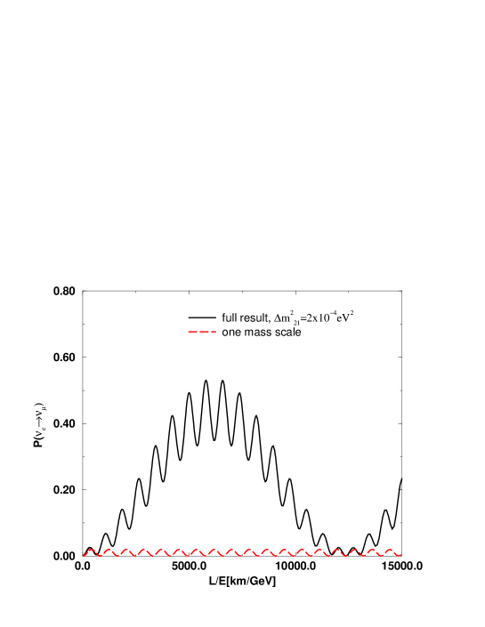
FIG. 1.: Plot of $P(\nu_{\mu}\to\nu_{e})$ as a function of $L/E$ for $\sin^{2}\theta_{23}=1$, $\Delta m^{2}_{32}=3\times 10^{-3}$ eV², $\sin^{2}2\theta_{12}=0.8$, and $\Delta m^{2}_{21}=2\times 10^{-4}$ eV², and $\sin^{2}2\theta_{13}=0.04$.

Even for the best-fit LMA solution, the effect of $\Delta m^{2}_{21}$ can be large for large pathlengths, and this would affect the $\nu_{\mu}\leftrightarrow\nu_{e}$ oscillations in atmospheric neutrino data, as shown in Fig. 2, for which we take the central values of $\sin^{2}2\theta_{21}$ and $\Delta m^{2}_{21}$ in the LMA fit, (40) and other parameters the same as in the previous figure. Note that for the dominant $\nu_{\mu}\to\nu_{\tau}$ transition in the atmospheric neutrinos, $\Delta m^{2}_{21}$ effects are not so important; this is clear from the fact that this transition does not directly involve $\nu_{e}$.

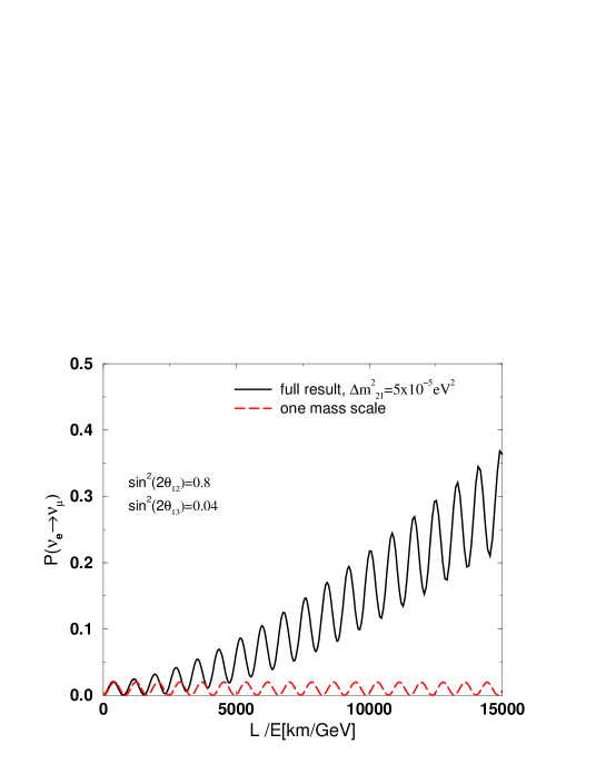
FIG. 2.: Plot of $P(\nu_{\mu}\to\nu_{e})$ as a function of $L/E$ for $\sin^{2}\theta_{23}=1$, $\Delta m^{2}_{32}=3\times 10^{-3}$ eV², central LMA values $\sin^{2}2\theta_{12}=0.8$ and $\Delta m^{2}_{21}=5\times 10^{-5}$ eV², and $\sin^{2}2\theta_{13}=0.04$.

We next show, in Fig. 3, the result of integrating (64) in the full three-flavor mixing scenario and using the actual density profile of the Earth as given in [35]. For this figure we use $\sin^{2}2\theta_{23}=1$, $\Delta m^{2}_{32}=3\times 10^{-3}$ eV², $\sin^{2}(2\theta_{12})=0.8$, $\Delta m^{2}_{21}=5\times 10^{-4}$ eV², and $\sin^{2}(2\theta_{13})=0.04$. As expected, the $\Delta m^{2}_{21}$ corrections are big for low energies and large distances. For the choice of a large distance, $L=10^{4}$ km (shown in fig. 3), we observe a very significant difference between the full calculation and the one-$\Delta m^{2}$ approximation. This shows again (as does the recent illustrative study in Ref. [18]), that it would be valuable to carry out a more complete analysis of the SuperK and other atmospheric neutrino data with not just three-flavor oscillations, but also two $\Delta m^{2}$ values included. Although the SuperK fit to its data shows that the $\nu_{\mu}\leftrightarrow\nu_{e}$ oscillations make a small contribution, it is important to include this contribution correctly, and the one-$\Delta m^{2}$ approximation is not, in general, reliable for this transition.

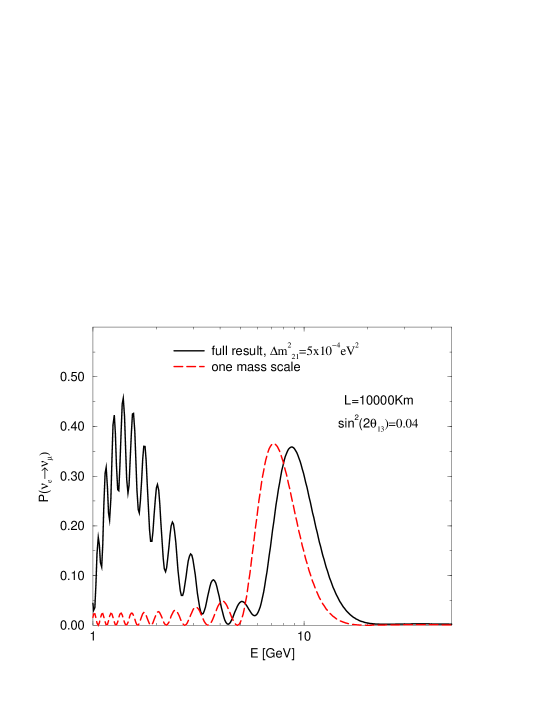
FIG. 3.: Plot of $P(\nu_{\mu}\to\nu_{e})$ as a function of $E$ for $\sin^{2}\theta_{23}=1$, $\Delta m^{2}_{32}=3\times 10^{-3}$ eV², and $L=10^{4}$Km, with other input values as shown. This calculation takes account of the full density profile of the earth.

VIII CP Violation

It is well known that there can be substantial leptonic CP violation observable in neutrino oscillations, in the context of three-flavor mixing and that this depends on both $\Delta m^{2}_{32}$ and $\Delta m^{2}_{21}$ being nonzero. The observation of leptonic CP violation is, indeed, a major goal of a neutrino factory [30]-[38]. Our main point here pertains to the accuracy with which input parameters might be known at a time when a neutrino factory might operate, which, in turn, leads one back to the necessity of a general three-flavor, two-$\Delta m^{2}$ analysis of atmospheric neutrino data and data from studies of $\nu_{\mu}\to\nu_{e}$ oscillations with an intense conventional neutrino beam. To elaborate on this, we recall that at a neutrino factory, a potentially promising way to measure CP violation is via the asymmetry

$$A_{1}=\frac{P(\nu_{e}\to\nu_{\mu})-P(\bar{\nu}_{e}\to\bar{\nu}_{\mu})}{P(\nu_{e}\to\nu_{\mu})+P(\bar{\nu}_{e}\to\bar{\nu}_{\mu})}$$ (78)

This method has two main appeals: (i) one can produce equally intense initial fluxes of $\nu_{e}$ and $\bar{\nu}_{e}$ by switching the stored beam between $\mu^{+}$ and $\mu^{-}$; and (ii) a detector for long-baseline neutrino oscillation searches with a neutrino factory will have the ability to identify outgoing $\mu^{\pm}$’s and measure their electric charges, and its detection efficiency will be equal for the two signs, so no bias will be introduced in this measurement. The complication with this method is that, even in the absence of any intrinsic CP violation, the asymmetry $A_{2}$ does not vanish because matter effects reverse sign between neutrino and antineutrinos, and the earth is not CP-symmetric. Therefore, the challenge with this method will be to determine these matter effects with sufficient accuracy to be able to disentangle them from the intrinsic CP violation. An important source of information here will be the anticipated measurement of $\theta_{13}$ from the JHF-SuperK experiment on $\nu_{\mu}\to\nu_{e}$ oscillations, since matter effects are sensitively dependent on this parameter [33]. As we have shown in a previous section, for an accurate determination of $\theta_{13}$, the one-$\Delta m^{2}$ approximation is not, in general, reliable, especially if $\sin^{2}2\theta_{21}$ and $\Delta m^{2}_{21}$ are near to their maximal values in the LMA solution to the solar neutrino deficit.

It should be noted that there are also plans to try to measure CP violation with an intense conventional beam, e.g. in the JHF-SuperK experimental program, by comparing overall rates of $\nu_{\mu}\to\nu_{e}$ and $\bar{\nu}_{\mu}\to\bar{\nu}_{e}$ and also energy dependences of these signals [26, 27] (see also [38]). For sufficiently large $\sin^{2}2\theta_{13}$, $\sin^{2}2\theta_{12}$, and $\Delta m^{2}_{21}$, these methods might provide a way to measure CP violation complementary to that used with a neutrino factory. There are a number of challenges with this approach: (i) the fluxes of $\nu_{\mu}$ and $\bar{\nu}_{\mu}$ are different; (ii) the event rates would involve several different cross sections, $\nu_{e}n\to e^{-}p$ and $\bar{\nu}_{e}p\to e^{+}n$ in oxygen nuclei, as well as $\bar{\nu}_{e}p\to e^{+}n$ on the hydrogen nuclei in the water molecules; (iii) since it is not possible to determine the sign of the $e^{\pm}$ with SuperK, the comparison would have to be done with data from different periods of operation. Assuming these experimental challenges can be met, the importance of accurate inputs for the various parameters is evident from the formula for the CP-violating asymmetry

$$A_{2}=\frac{P(\nu_{\mu}\to\nu_{e})-P(\bar{\nu}_{\mu}\to\bar{\nu}_{e})}{P(\nu_{\mu}\to\nu_{e})+P(\bar{\nu}_{\mu}\to\bar{\nu}_{e})}$$ (79)

For the JHF-SuperK baseline matter effects are small, so we shall consider the expression for this asymmetry in vacuum (where $A_{2}=-A_{1}$). Using

$$P(\nu_{\mu}\to\nu_{e})-P(\bar{\nu}_{\mu}\to\bar{\nu}_{e}) = 4J(\sin 2\phi_{32}+\sin 2\phi_{21}+\sin 2\phi_{13})$$ (80)

$$= 16J\sin\phi_{32}\sin\phi_{31}\sin\phi_{21}$$ (81)

where $J$ was given in eq. (3), substituting the expression for $P(\nu_{\mu}\to\nu_{e})+P(\bar{\nu}_{\mu}\to\bar{\nu}_{e})$ from (46), and using $\Delta m^{2}_{21}<<\Delta m^{2}_{32}$, one has

$$A_{2}\simeq\frac{\sin(2\theta_{12})\cot\theta_{23}\sin\delta\sin\phi_{21}}{\sin\theta_{13}}$$ (82)

Thus, to extract an accurate measurement of $\sin\delta$, it is clearly important to have sufficiently accurate inputs for quantities such as $\theta_{13}$, and this, in turn, motivates the generalization of the one-$\Delta m^{2}$ approximation that we have presented above for the analysis of data on neutrino oscillations.

IX Conclusions

In this paper we have performed calculations of neutrino oscillation probabilities in a three-flavor context, taking into account both $\Delta m^{2}_{atm}$ and $\Delta m^{2}_{sol}$ scales. We have shown that for values of $\sin^{2}(2\theta_{13})\sim 10^{-2}$ in the range of interest for long-baseline neutrino oscillation experiments with intense conventional neutrino beams such as JHF-SuperK and with a possible future neutrino factory, and for $\Delta m^{2}_{sol}\sim 10^{-4}$ eV², the contributions to $\nu_{\mu}\to\nu_{e}$ oscillations from both CP-conserving and CP-violating terms involving $\sin^{2}(\Delta m^{2}_{sol}L/(4E))$ can be comparable to the terms involving $\sin^{2}(\Delta m^{2}_{atm}L/(4E))$ retained in the one-$\Delta m^{2}$ approximation. Accordingly, we have emphasized the importance of performing a full three-flavor, two-$\Delta m^{2}$ analysis of the data on $\nu_{\mu}\to\nu_{e}$ oscillations from an experiment with a conventional beam, and on $\nu_{e}\to\nu_{\mu}$, $\bar{\nu}_{e}\to\bar{\nu}_{\mu}$ oscillations from experiments with a neutrino factory. In our study we have included calculations of matter effects in a three-flavor, two $\Delta m^{2}$ framework. Our results also motivate the analysis of atmospheric neutrino data in this generalized framework.

Acknowledgments

This research was supported in part by the U. S. NSF grant PHY-97-22101.

X Appendix: Analytic Approximation for Three-Flavor Two-$\Delta{m}^{2}$ Oscillations in Matter

In matter, for constant density, it is still possible to solve the evolution equation exactly ([36]). However, these results are rather complicated. For fits to the data or other studies, it can be useful in this case to use approximate formulas that can still very well describe the oscillations.

For the LMA solution to the solar data, the effects of $\Delta m^{2}_{sol}$ can no longer be neglected, but there are cases where they are small in long-baseline experiments for which the dominant oscillation is controlled by $\Delta m^{2}_{atm}$. In these cases, one can thus treat the effects of $\Delta m^{2}_{sol}$ as a small perturbation. This has been done in [37], where the matter effect is also take to be a small perturbation. This is a good approximation at short and medium distances. Here we give generalized formulas that treat the $\Delta m^{2}_{sol}$ as a perturbation but allow large matter effects, as is necessary in very long baseline experiments.

In order to calculate oscillation probabilities it is now convenient to work in a basis defined by:

$$\nu=UR_{12}^{\dagger}\nu^{\prime}$$ (83)

The evolution of $\nu^{\prime}$ is given by

$$H^{\prime} = R_{12}U^{\dagger}HUR_{12}^{\dagger}$$ (84)

$$= \frac{\Delta m_{atm}^{2}}{2E}\pmatrix{0&0&0\cr 0&0&0\cr 0&0&1}+R_{12}U^{\dagger}VUR_{12}^{\dagger}+\frac{\Delta m^{2}_{sol}}{2E}R_{12}\pmatrix{0&0&0\cr 0&1&0\cr 0&0&1}R_{12}^{\dagger}$$ (85)

$$= \pmatrix{V_{e}c_{13}^{2}&0&V_{e}c_{13}s_{13}e^{-i\delta}\cr 0&0&0\cr V_{e}c_{13}s_{13}e^{i\delta}&0&V_{e}s_{13}^{2}+\frac{\Delta m_{atm}^{2}}{2E}&}+\frac{\Delta m^{2}_{sol}}{2E}\pmatrix{s_{12}^{2}&s_{12}c_{12}&0\cr s_{12}c_{12}&c_{12}^{2}&0\cr 0&0&1}$$ (86)

From this we obtain $\nu^{\prime}(x)=S^{\prime}\nu^{\prime}(0)$, with

$$S^{\prime}=e^{-iDL}\pmatrix{\cos{\big{(}\frac{\omega^{\prime}L}{2}\big{)}}+\frac{i}{\omega^{\prime}}A^{\prime}\sin{\big{(}\frac{\omega^{\prime}L}{2}\big{)}}&0&-\frac{i}{\omega^{\prime}}B^{\prime}e^{-i\delta}\sin{\big{(}\frac{\omega^{\prime}L}{2}\big{)}}\cr 0&e^{iDL}&0\cr-\frac{i}{\omega^{\prime}}B^{\prime}e^{i\delta}\sin{\big{(}\frac{\omega^{\prime}L}{2}\big{)}}&0&\cos{\big{(}\frac{\omega^{\prime}L}{2}\big{)}}-\frac{i}{\omega^{\prime}}A^{\prime}\sin{\big{(}\frac{\omega^{\prime}L}{2}\big{)}}}+\frac{\Delta m^{2}_{sol}}{2E}S^{\prime}_{c}$$ (87)

The first term gives the one-$\Delta m^{2}$ contribution, which, after the rotation to the flavor basis $(\nu_{e},\nu_{\mu},\nu_{\tau})$, is the same as the one obtained in the previous section. The second term contains the corrections due to the $\Delta m^{2}_{sol}$ term. $S^{\prime}_{c}$ is given by

$${S^{\prime}_{c}}_{11}=e^{-iDL}\bigg{[}L\frac{A^{\prime}}{\omega^{\prime}}s_{12}^{2}\sin{\big{(}\frac{\omega^{\prime}L}{2}\big{)}}+i\bigg{(}c_{12}^{2}\frac{B^{\prime 2}}{\omega^{\prime 3}}\sin{\big{(}\frac{\omega^{\prime}L}{2}\big{)}}-\frac{L}{2}\bigg{(}1+s_{12}^{2}-c_{12}^{2}\frac{A^{\prime 2}}{2\omega^{\prime 2}}\bigg{)}\cos{\big{(}\frac{\omega^{\prime}L}{2}\big{)}}\bigg{)}\bigg{]}$$ (88)

$${S^{\prime}_{c}}_{22}=0$$ (89)

$${S^{\prime}_{c}}_{33}=e^{-iDL}\bigg{[}-L\frac{A^{\prime}}{\omega^{\prime}}\sin{\big{(}\frac{\omega^{\prime}L}{2}\big{)}}-i\bigg{(}c_{12}^{2}\frac{B^{\prime 2}}{\omega^{\prime 3}}\sin{\big{(}\frac{\omega^{\prime}L}{2}\big{)}}+L\frac{1}{2}\bigg{(}1+s_{12}^{2}+c_{12}^{2}\frac{A^{\prime 2}}{2\omega^{\prime 2}}\bigg{)}\cos{\big{(}\frac{\omega^{\prime}L}{2}\big{)}}\bigg{)}\bigg{]}$$ (90)

$${S^{\prime}_{c}}_{12}=\frac{2Es_{12}c_{12}}{\Delta m^{2}_{atm}V_{e}c_{13}^{2}}\bigg{[}(V_{e}c_{13}^{2}-2D)+e^{-iDL}\bigg{(}(2D-V_{e}c_{13}^{2})\cos{\big{(}\frac{\omega^{\prime}L}{2}\big{)}}+i\frac{\omega^{\prime 2}+2A^{\prime}D}{2\omega^{\prime}}\sin{\big{(}\frac{\omega^{\prime}L}{2}\big{)}}\bigg{)}\bigg{]}$$ (91)

$${S^{\prime}_{c}}_{13}=\frac{V_{e}c_{13}s_{13}e^{-i\delta}}{\omega^{\prime}}e^{-iDL}\bigg{[}L(1+s_{12}^{2})\sin{\big{(}\frac{\omega^{\prime}L}{2}\big{)}}+ic_{12}^{2}\frac{A^{\prime}}{\omega^{\prime}}\bigg{(}\frac{2}{\omega^{\prime}}\sin{\big{(}\frac{\omega^{\prime}L}{2}\big{)}}-L\cos{\big{(}\frac{\omega^{\prime}L}{2}\big{)}}\bigg{)}\bigg{]}$$ (92)

$${S^{\prime}_{c}}_{23}=\frac{2E}{\Delta m^{2}_{atm}}{s_{12}c_{12}}{\rm tg}\theta_{13}e^{-i\delta}\bigg{[}1-e^{-iDL}\bigg{(}\cos{\big{(}\frac{\omega^{\prime}L}{2}\big{)}}+2i\frac{D}{\omega^{\prime}}\sin{\big{(}\frac{\omega^{\prime}L}{2}\big{)}}\bigg{)}\bigg{]}$$ (93)

$${S^{\prime}_{c}}_{21}={S^{\prime}_{c}}_{12},\,\,\,\,{S^{\prime}_{c}}_{31}=e^{2i\delta}{S^{\prime}_{c}}_{13},\,\,\,\,{S^{\prime}_{c}}_{32}=e^{2i\delta}{S^{\prime}_{c}}_{23}$$ (94)

with

$$A^{\prime}=\frac{\Delta m_{atm}^{2}}{2E}-{\sqrt{2}}G_{F}N_{e}\cos(2\theta_{13})$$ (95)

$$B^{\prime}=V_{e}\sin(2\theta_{13})$$ (96)

$$\omega^{\prime}=\sqrt{A^{\prime 2}+B^{\prime 2}}=\bigg{[}\bigg{(}V_{e}\cos(2\theta_{13})-\frac{\Delta m_{atm}^{2}}{2E}\bigg{)}^{2}+V_{e}^{2}\sin^{2}(2\theta_{13})\bigg{]}^{1/2}$$ (97)

After we rotate back in the actual flavor basis, the oscillation probabilities will be given by

$$P(\nu_{a}\to\nu_{b})=|(UR_{12}^{\dagger}S^{\prime}R_{12}U^{\dagger})_{ab}|^{2}$$ (98)

The results from Eq. (98) are compared in Fig. 4, 5 with those obtained from the exact numerical result and with the result for the one-$\Delta m^{2}$ approximation for the following set of input values: $\sin^{2}2\theta_{23}=1$, $\Delta m^{2}_{32}=3\times 10^{-3}$ eV², $\sin^{2}2\theta_{sol}=\sin^{2}2\theta_{12}=.8$ and $\Delta m^{2}_{sol}=\Delta m^{2}_{21}=10^{-4}$eV² (or $\Delta m^{2}_{sol}=0$ for comparison), and $\sin^{2}2\theta_{13}=0.04$.

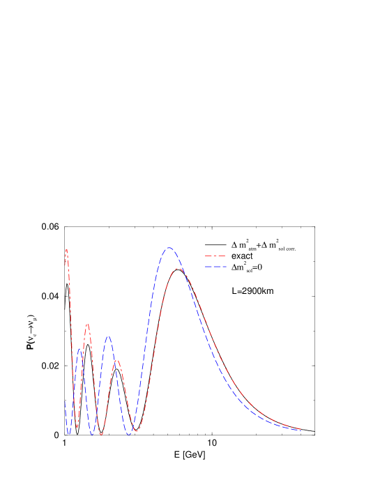
FIG. 4.: Plot of $P(\nu_{e}\to\nu_{\mu})$ as a function of $E$ for $L=2900$ km. Other input parameter values are given in the text.

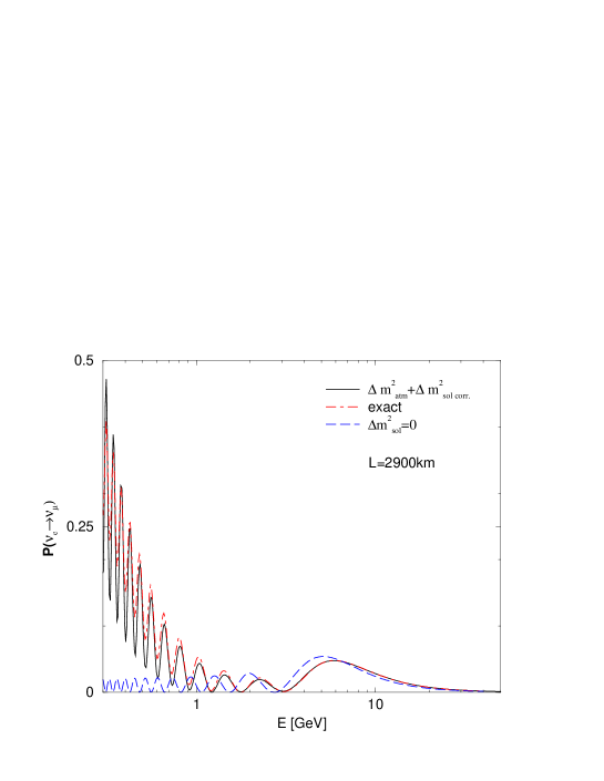
FIG. 5.: Plot of $P(\nu_{e}\to\nu_{\mu})$ as a function of $E$ for $L=2900$ km, with detail of the region from $E=0$ to $E=1$ GeV. Input parameter values are given in the text.

REFERENCES

- [1] Homestake: B.T. Cleveland et al, Astrophys.J. 496, 505 (1998); Kamiokande: K. Hirata et al., Phys. Rev. D44, 2241 (1991); SAGE: J. N. Abdurashitov al., Phys. Rev. C60, 055801 (1999); GALLEX: Hampel et al., Phys. Lett. B447, 127 (1999); GNO: M. Altmann et al., Phys.Lett.B490, 16 (2000); Superkamiokande: Y. Fukuda et al., Phys. Rev. Lett. 82, 1810, 243 (1999); Phys. Rev. Lett. 86, 5651, 5656 (2001); SNO: . Q. Ahmad et al., Phys. Rev. Lett. 87, 071301 (2001).
- [2] In addition to the fits given by experimentalists themselves, there are numerous fits by theorists; a few recent ones are J. Bahcall, P. Krastev, and A. Smirnov, Phys. Rev. D60, 093001 (1999); JHEP 0105, 015 (2001); M. C. Gonzalez-Garcia, M. Maltoni, C. Peña-Garay, and J. W. F. Valle, Phys. Rev. D63, 033005 (2001); J. N. Bahcall, M. C. Gonzalez-Garcia, C. Pena-Garay, hep-ph/ hep-ph/0106258; P. Krastev, A. Smirnov, hep-ph/0108177; G. L. Fogli, E. Lisi, A. Marrone, D. Montanino, A. Palazzo, hep-ph/0104221; G. L. Fogli, E. Lisi, and A. Palazzo, hep-ph/0105080; S. Choubey, S. Goswami, N. Gupta, D. P. Roy, hep-ph/0103318.
- [3] M.V. Garzelli, C. Giunti,hep-ph/0007155; R. Barbieri, A. Strumia, JHEP 0012, 016 (2000); P. Creminelli, G. Signorelli, A. Strumia, JHEP 0105:052 (2001); V. Barger, D. Marfatia, K. Whisnant, B.P. Wood, Phys. Rev. D64 073009 (2001).
- [4] L. Wolfenstein, Phys. Rev. D17, 2369 (1978); S. P. Mikheyev and A. Smirnov, Yad. Fiz. 42, 1441 (1985) [Sov.J. Nucl. Phys. 42, 913 (1986)], Nuovo Cim., C9, 17 (1986); S. P. Rosen and J. Gelb, Phys. Rev. D34, 969 (1986); S. Parke, Phys. Rev. Lett. 57, 1275 (1986); W. Haxton, Phys. Rev. Lett. 57, 1271 (1986); J. Pantaleone and T. K. Kuo, Rev. Mod. Phys. 61, 937 (1989).
- [5] K. S. Hirata et al., Phys. Lett. B205, 416; ibid. 280, 146 (1992); Y.Fukuda et al., Phys. Lett. B335, 237 (1994); S. Hatakeyama et al. Phys. Rev. Lett. 81, 2016 (1998).
- [6] D. Casper et al., Phys. Rev. Lett. 66, 2561 (1991); R.Becker-Szendy et al., Phys. Rev. D46, 3720 (1992); Phys. Rev. Lett. 69, 1010 (1992).
- [7] W. Allison et al., Phys. Lett. B391, 491 (1997); Phys. Lett. B449, 137 (1999); W. A. Mann, Nucl. Phys. Proc. Suppl. 91, 134 (2000).
- [8] Y. Fukuda et al., Phys. Lett. B433, 9 (1998); Phys. Lett. B436, 33 (1998). Y. Fukuda et al., Phys. Lett. B467, 185 (1999); Phys. Rev. Lett. 82, 2644 (1999); C. McGrew, in the Workshop on Neutrino Telescopes, Venice (Mar., 2001); C. Yanagisawa, in Frontiers in Contemporary Physics (Vanderbilt Univ., Mar. 2001); T. Toshito, in the Recontres de Moriond (Mar., 2001).
- [9] MACRO Collab., M. Ambrosio et al., Phys. Lett. B478, 5 (2000); hep-ex/0001044; B. Barish, Nucl. Phys. Proc. Suppl. 91, 141 (2000); hep-ex/0101019.
- [10] M. Apollonio et al., Phys. Lett. B420, 397 (1998); Phys. Lett. B466, 415 (1999).
- [11] F. Boehm et al., Phys. Rev. Lett. 84, 3764 (2000); Phys. Rev.D62, 072002 (2000).
- [12] S. Ahn et al., Phys. Lett. B511, 178 (2001); J. Hill, talk at Snowmass-2001.
- [13] C. Athanassopoulous et al., Phys. Rev. Lett. 77, 3082 (1996); Phys. Rev. Lett. 81, 1774 (1998); A. Aguilar et al., hep-ex/0104049.
- [14] K. Eitel (for KARMEN Collab.), Nucl. Phys. Proc. Suppl. 91, 191 (2000).
- [15] If one were also to fit the LSND data, one would be led to include light electroweak-singlet neutrinos. Since the LSND experiment has not so far been confirmed, we shall not try to include the LSND data in our discussion.
- [16] A. Baltz, A. S. Goldhaber, M. Goldhaber, Phys. Rev. Lett. 81, 5730 (1998).
- [17] G. L. Fogli, E. Lisi, A. Marrone, G. Scioscia, Phys. Rev. D59, 033001 (1998); C. W. Kim, U.W. Lee, Phys. Lett. B444, 204 (1998); C. Giunti, , C. W. Kim, U. W. Lee, V.A. Naumov, hep-ph/9902261; O. Peres, A. Yu. Smirnov, Phys. Lett. B456, 204 (1999); A. Strumia, JHEP 9904,026 (1999).
- [18] G. L. Fogli, E. Lisi, and A. Marrone, Phys. Rev. D64, 093005 (2001).
- [19] G. Barenboim, A. Dighe, and S. Skadhauge, hep-ph/0106002.
- [20] C. Jarlskog, Z. Phys. C29, 491 (1985); Phys. Rev. D35, 1685) (1987).
- [21] A. de Gouvea, A. Friedland and H. Murayama, Phys. Lett. B490, 125 (2000).
- [22] See, e.g., J. Busenitz et al., Proposal for U.S. Participation in KamLAND (Mar. 1999). In addition to the reactor oscillation search, this experiment also intends to measure solar 7Be neutrinos.
- [23] V. Barger, D. Marfatia, and B. Wood, Phys. Lett. B498, 53 (2001); H. Murayama, hep-ph/0012075.
- [24] See http://www.hep.anl.gov/ndk/hypertext/minos.html.
- [25] See http://proj-cngs.web.cern.ch/proj-cngs/.
- [26] For information on the JHF-SuperK project and possible upgrades involving a more intense beam and the construction of a 1 Mton water Cherenkov far detector (HyperKamiokande), see http://neutrino.kek.jp/jhfnu, in particular, Y. Itoh et al., “Letter of Intent: A Long Baseline Neutrino Oscillation Experiment using the JHF 50 GeV Proton Synchrotron and the Super-Kamiokande Detector” (Feb. 2000); Y. Itoh et al, “The JHF-Kamioka Neutrino Project”.
- [27] V. Barger et al. (Fermilab Superbeam Working Group), Nov., 2000, hep-ph/0103052; Phys. Rev. D63, 113011 (2001); D. Harris, talk at UNO workshop (Aug. 2000), R. Shrock, talks at UNO workshop, June, 2001; http://superk.physics.sunysb.edu/uno; J. Cadenas et al. (CERN Superbeam Working Group), hep-ph/0105297. Some possibilities include a second detector (perhaps off-axis) as an extension of the MINOS experiment, and options involving FNAL-Homestake, BNL-Ithaca, BNL-Homestake, CERN-Frejus, or JHF-Beijing.
- [28] References and websites for these experiments and future projects can be found, e.g., at http://www.hep.anl.gov/ndk/hypertext/nu_industry.html.
- [29] S. Geer, Phys. Rev. D57, 6989 (1998).
- [30] C. Albright et al. (Fermilab Neutrino Factory Physics Working Group), “Physics at a Neutrino Factory”, Apr. 2000, hep-ph/hep-ex/0008064. See also the companion machine study “Feasibility Study of a Neutrino Factory Based on a Muon Storage Ring”, by the Fermilab Neutrino Factory Feasibility Study Working Group, N. Holtkamp, et al.
- [31] Muon Collider and Neutrino Factory Collaboration, “Neutrino Factory Feasibility Study II” (May 2001), available at http://www.cap.bnl.gov/mumu.
- [32] See, e.g., http://www.fnal.gov/projects/muon_collider/nu/study/study.html http://www.cern.ch/~autin/nufact99/whitepap.ps http://www.cap.bnl.gov/mumu http://puhep1.princeton.edu/mumu/NSFLetter/nsfmain.ps.
- [33] V. Barger, K. Whisnant, S. Pakvasa, and R. J. N. Phillips, Phys. Rev. D22, 2718 (1980); P. Krastev, Nuovo Cimento 103A, 361 (1990); R. H. Bernstein and S. J. Parke, Phys. Rev. D44, 2069 (1991); De Rujula, M. B. Gavela, and P. Hernandez, Nucl. Phys. B547, 21 (1999); P. Lipari, Phys.Rev. D61, 113004 (2000) S. Dutta, R. Gandhi, and B. Mukhopadhyaya, Eur.Phys.J. C18, 405 (2000); V. Barger, S. Geer, K. Whisnant, Phys.Rev. D61, 053004 (2000); D. Dooling, C. Giunti, K. Kang, C. W. Kim,Phys.Rev. D61,073011 (2000); A. Bueno, M. Campanelli, A. Rubbia, Nucl.Phys. B573, 27 (2000); V. Barger, S. Geer, R. Raja, K. Whisnant, Phys.Rev. D62, 013004 (2000); M. Freund, M. Linder, S.T. Petcov, A. Romanino, Nucl.Phys. B578, 27 (2000); I. Mocioiu and R. Shrock, AIP Conf.Proc. 533, 74 (2000) (NNN99); I. Mocioiu and R. Shrock, Phys.Rev. D62, 053017 (2000); V. Barger, S. Geer, R. Raja, K. Whisnant, Phys.Rev. D62, 073002 (2000); A. Cervera, A. Donini, M.B. Gavela, J. Gomez Cadenas, P. Hernandez, O. Mena, and S. Rigolin, Nucl.Phys. B579, 17 (2000), Erratum-ibid. B593, 731 (2001); M. Freund, P. Huber, M. Lindner, Nucl.Phys. B585, 105 (2000); V. Barger, S. Geer, R. Raja, K. Whisnant, Phys.Lett. B485, 379 (2000); Z.-Z. Xing, Phys. Lett. 487, 327 (2000); Phys. Rev. D63, 073012 (2000); A. Bueno, M. Campanelli, A. Rubbia, Nucl.Phys. B589, 577 (2000); P. Fishbane, Phys. Rev. D62, 093009 (2000); P. Fishbane and P. Kaus, Phys. Lett. B506, 275 (2001); P. Fishbane and S. Gasiorowicz, hep-ph/0012230; V. Barger, S. Geer, R. Raja, K. Whisnant, Phys.Rev. D63, 033002 (2001); M. Freund, P. Huber, M. Lindner, hep-ph/0105071.
- [34] E. Akhmedov, A. Dighe, P. Lipari, A. Smirnov, Nucl. Phys. B542, 3 (1999); E. Akhmedov, Nucl.Phys. B538, 25 (1999); E. Akhmedov, hep-ph/0001264; E. Akhmedov, P. Huber, M. Lindner, and T. Ohlsson, Nucl. Phys. B608, 394 (2001).
- [35] A.Dziewonski, Earth Structure, in: ”The Encyclopedia of Solid Earth Geophysics”, D.E.James (Ed.), (Van Nostrand Reinhold, New York, 1989), p.331.
- [36] See, e.g., H. Zaglauer, K. Schwarzer, Z. Phys. C40, 273 (1988); T. Ohlsson, H. Snellman, J. Math. Phys. 41, 2768 (2000).
- [37] J. Arafune, J. Sato, Phys.Rev. D55, 1653 (1997); H. Minakata, H. Nunokawa, Phys.Rev. D57, 4403 (1998); M. Koike, J. Sato, Phys. Rev. D62, 073006 (2000);
- [38] S.M. Bilenky, C. Giunti, W.Grimus, Phys.Rev. D58, 033001 (1998); K. Dick, M. Freund, M. Lindner, A. Romanino, Nucl. Phys. B562, 29 (1999); M. Tanimoto, Phys. Lett. B462, 115 (1999); A. Donini, M.B. Gavela, P. Hernandez, S. Rigolin, Nucl.Phys. B574, 23 (2000); A. Romanino, Nucl.Phys. B574 675 (2000); M. Koike, J. Sato, Phys.Rev. D61, 073012 (2000), Erratum-ibid. D62, 079903 (2000); S. J. Parke, T. J. Weiler, Phys.Lett. B501, 106 (2001); T. Miura, E. Takasugi, Y. Kuno, and M. Yoshimura, Phys. Rev. D64, 013002 (2001); M. Koike, T. Ota, J. Sato, hep-ph/0011387; P. Lipari. hep-ph/0102046.