Dark energy from the Trans-Planckian physics

As yet, there is no underlying fundamental theory for the transplanckian regime. There is a need to address the issue of how the observables in our present Universe are affected by processes that may have occurred at superplanckian energies (referred to as the transplanckian regime). Specifically, we focus on the impact the transplanckian regime has on the dark energy. We model the transplanckian regime by introducing a 1-parameter family of smooth non-linear dispersion relations which modify the frequencies at very short distances. A particular feature of the family of dispersion functions chosen is the production of ultralow frequencies at very high momenta $k$ (for $k>M_{P}$). We show that the range of modes with frequencies equal or less than the current Hubble rate $H_{0}$ which are still frozen today provides a strong candidate for the dark energy of the Universe.

1 Introduction

There is strong evidence our Universe is accelerating due to a nearly constant vacuum energy, the dark energy, that accounts for about 70% of the present total energy density. Although the SN1a data indicating acceleration is inconclusive, the observed CMB spectrum ($\Omega_{0}\simeq 1.1\pm 0.07$) as well as the measurements of the Hubble constant (i.e. the age of the Universe) strongly support the case of a universe with a large dark energy component [1]. There are many efforts in 4 or higher dimensional models that address the issue of producing such a small vacuum energy from the cosmological fundamental mass scale. An equally challenging question is why the dark energy is the dominant component today . From the particle physics point of view, the main task is to explain why its value is $10^{-122}$ in units of the Planck mass $M_{P}$. Generally in these efforts, either a large amount of fine-tuning, or the introduction of some ad-hoc, unnaturally small parameter is required.

We propose in this talk a new approach for the origin of dark energy, which is based on contributions from the transplanckian regime. This alternative model makes use of the ‘freeze-out by expansion‘ mechanism of a range of modes in the transplanckian regime that contribute the correct amount to the dark energy of the universe, without any fine-tuning and with $M_{pl}$ as the fundamental scale of the theory [2].

In an expanding universe, the physical momenta are blueshifted back in time; therefore some of the observed low values of the momenta today that contribute to the CMBR spectrum may have originated from the transplanckian regime in the Early Universe. Similar issues apply to the Hawking radiation in Black Hole physics. In a series of papers [3], it was demonstrated that the Hawking radiation remains unaffected by modifications of the ultra high energy regime, expressed through the modification of the usual linear dispersion relation at energies larger than a certain ultraviolet scale $k_{C}$. Following a similar procedure, in the case of an expanding Friedmann-Lemaitre-Robertson-Walker (FLRW) spacetime, it has been showed [4, 2] that the primordial scale invariant power spectrum can be recovered if the dispersion relation for the metric perturbations is a smooth function such that it gives rise to an adiabatic time-evolution of the modes.

We incorporate the concept of superstring duality (which applies at transplanckian regimes) in the family of dispersion models for the transplanckian regime below [2] by choosing a particular family of dispersion relations that exhibits dual behavior, i.e. appearance of ultra-low mode frequencies both at low and high momenta $k$.

2 Dark Energy from the “Tail”

Let us start with the generalized Friedmann-Lemaitre-Robertson-Walker (FLRW) line-element which, in the presence of scalar and tensor perturbations, takes the form [6]

$$ds^{2} = a^{2}(\eta)\left\{-d\eta^{2}+\left[\delta_{ij}+h(\eta,{\bf n})Q\delta_{ij}\right.\right.$$ (1)

$$\left.\left.+h_{l}(\eta,{\bf n})\frac{Q_{ij}}{n^{2}}+h_{gw}(\eta,{\bf n})Q_{ij}\right]dx^{i}dx^{j}\right\}\,,$$

where $\eta$ is the conformal time and $a(\eta)$ the scale factor. The dimensionless quantity ${\bf n}$ is the comoving wavevector, related to the physical vector ${\bf k}$ by ${\bf k}={\bf n}/a(\eta)$ as usual. The functions $h$ and $h_{l}$ represent the scalar sector of perturbations while $h_{gw}$ represents the gravitational waves. $Q(x^{i})$ and $Q_{ij}(x^{i})$ are the eigenfunction and eigentensor, respectively, of the Laplace operator on the flat spacelike hypersurfaces. For simplicity, we will take a scale factor $a(\eta)$ given by a power law, $a(\eta)=|\eta_{c}/\eta|^{\beta}$, where $\beta\geq 1$ and $|\eta_{c}|=\beta/H(\eta_{c})$. The initial power spectrum of the perturbations can be computed once we solve the time-dependent equations in the scalar and tensor sector. The mode equations for both sectors reduce [6] to a Klein-Gordon equation of the form

$$\mu_{n}^{\prime\prime}+\left[n^{2}-\frac{a^{\prime\prime}}{a}\right]\mu_{n}=0\,,$$ (2)

where the prime denotes derivative with respect to conformal time. Therefore, studying perturbations in a FLRW background is equivalent to solving the mode equations for a scalar field $\mu$ related to the perturbation field in the expanding background.

In what follows, we replace the linear relation $\omega^{2}(k)=k^{2}=n^{2}/a(\eta)^{2}$ with a nonlinear dispersion relation (which is the class of Epstein functions) $\omega(k)=F(k)$, such that

$$n_{eff}^{2}=a(\eta)^{2}F(k)^{2}=n^{2}\left(\frac{\epsilon_{1}}{1+e^{x}}+\frac{\epsilon_{2}e^{x}}{1+e^{x}}+\frac{\epsilon_{3}e^{x}}{(1+e^{x})^{2}}\right)\,,$$ (3)

where $x=(k/k_{C})^{1/\beta}=A|\eta|$, with $A=(1/|\eta_{c}|)(n/k_{C})^{1/\beta}$. This dispersion function encapsulates the T-duality behaviour.Then, the equation for the scalar and tensor perturbations, that we need to solve, takes the form

$$\mu_{n}^{\prime\prime}+\left[n^{2}_{eff}-(1-6\xi)\frac{a^{\prime\prime}}{a}\right]\mu_{n}=0\,.$$ (4)

This equation represents particle production in a time-dependent background. We use the method of Bogolubov transformation to calculate the spectrum of particles created and their energy. Although at late time the background is asymptotically flat, the wavefunction will be in a squeezed state due to the curved background that mixes positive and negative frequencies. The evolution of the mode function $\mu_{n}$ at late times fixes the Bogolubov coefficients $\alpha_{n}$ and $\beta_{n}$,

$$\mu_{n}\rightarrow_{\eta\rightarrow+\infty}\frac{\alpha_{n}}{\sqrt{2\Omega^{out}_{n}}}e^{-i\Omega^{out}_{n}\eta}+\frac{\beta_{n}}{\sqrt{2\Omega^{out}_{n}}}e^{+i\Omega^{out}_{n}\eta}\,,$$ (5)

with $|\beta_{n}|^{2}$ being the Bogolubov coefficient equal to the particle creation number per mode $n$, and $\Omega^{out}_{n}\simeq\sqrt{\epsilon_{1}}n$. Using the linear transformation properties of hypergeometric functions, we find that

$$\left|\frac{\beta_{n}}{\alpha_{n}}\right| = e^{-2\pi\tilde{b}}\left|\frac{\cosh\pi(\tilde{d}+\tilde{b})}{\cosh\pi(\tilde{d}-\tilde{b})}\right|\,,$$ (6)

where $\tilde{b}$ and $\tilde{d}$ are given in terms of the Epstein parameters [2] $\epsilon_{i}$.

The family of of our dispersion models, for the frequency $n_{eff}$ , Fig. 1, attenuates to zero in the transplanckian regime ($\epsilon_{2}=0$), thereby producing ultralow frequencies at very short distances. Details about the exact solutions to the mode equations and the spectrum computed through the method of Bogolubov coefficients can be found in Ref. [2]. The resulting CMBR spectrum is shown to be (nearly) that of a black body, i.e., (nearly) scale invariant. Below we concentrate on the energy contained in the ultralow frequencies range of modes, and show that it is of the same order today as the matter energy density.

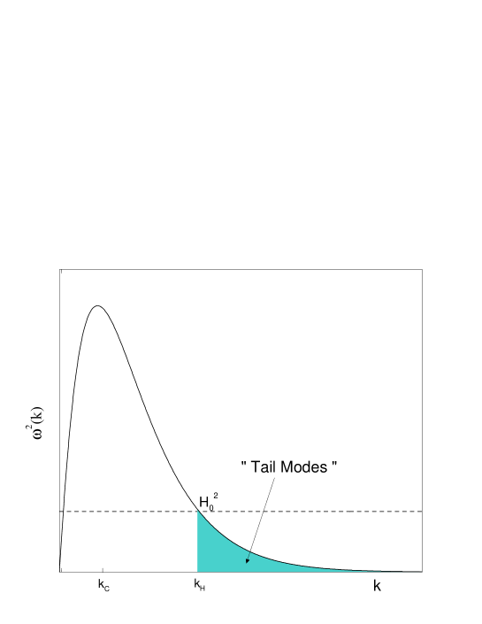
Figure 1: Dispersion function and the range of modes in the tail, $k_{H}<k<\infty$. $H_{0}$ is the present value of the Hubble constant.

For the special features of our choice of dispersion relation Eq. (3), it is straightforward to calculate: i) which of the transplanckian modes have always been frozen to the present time and ii) the energy density contained in these modes. The modes at very high momenta but of ultra low frequencies $\omega(k)$ are frozen for as long as the Hubble expansion rate $H$ of the Universe dominates over their frequency. We refer to that as the $tail$ of the dispersion graph. In Fig. (1), for the dispersed $\omega^{2}(k)$ vs. $k$, the tail corresponds to all the modes beyond the point $k_{H}$, where $k_{H}$ is derived by the condition $\omega^{2}(k_{H})=H^{2}_{0}$, and $H_{0}$ is the Hubble rate today. It then follows that they have not decayed and redshifted away but are still frozen $today$. On the other hand, since $H$ has been a decreasing function of time, many modes, even those in the ultralow frequency range, have become dynamic and redshifted away one by one, every time the expansion rate $H$ dropped below their frequency. Clearly, these modes have long decayed into radiation, and the tail modes are the only modes still frozen. They contain vacuum energy of very short distance, hence of very low energy. The last mode in the tail would decay when and if $H=0$. Their time-dependent behavior when they decay depends on the evolution of $H$ and is complicated because they contribute to the expansion rate for $H$.

However we can calculate their contribution to the dark energy today, when they are still frozen, thereby mimicking a cosmological constant. The energy for the tail is given by:

$$\langle\rho_{tail}\rangle=\frac{1}{2\pi^{2}}\int^{\infty}_{k_{H}}kdk\int\omega(k)d\omega~{}|\beta_{k}|^{2}\,,$$ (7)

where the $|\beta_{k}|^{2}$ coefficient can be found in Ref. [2]. We would also like to stress that due to the dispersion class of functions chosen (defined in the whole range of momenta from zero to infinity) the total energy contribution of the modes produced is finite, and the zero-point vacuum energy (the global cosmological cosntant) vanishes without the need of applying any renormalization/subtraction scheme. In a sense, the regularization-renormalization procedure is encoded in the class of dispersions we postulate.

The numerical calculation of the tail energy produced the following result: for random different values of the free parameters, the dark energy of the tail is $\rho_{tail}=10^{-122}f(\epsilon_{1})$, times less than the total energy during inflation, i.e. $\frac{\rho_{tail}}{\rho_{total}}=10^{-122}f(\epsilon_{1})$ at Planck time. The prefactor $f(\epsilon_{1})$, which depends weakly on the parameter of the dispersion family $\epsilon_{1}$, is a small number between 1 to 9, which clearly can contribute at the most by 1 order of magnitude.

This $amazing$ result can be understood qualitatively by noticing that the behavior of the frequency for the “tail” modes is nearly an exponential decay (see Eq. (3)), and as such dominates over the other terms in the energy integrand of Eq. (7):

$$\omega^{2}(k>k_{C})\approx exp(-k/k_{C})\,,$$ (8)

Hence, due to the decaying exponential, the main contribution to the energy integral in Eq. (7) comes from the highest value of this exponentially decaying frequency, which is the value of the integrand at the tail starting point, $k_{H}\sim O(M_{P})$, i.e.,

$$\langle\frac{\rho_{tail}}{\rho_{total}}\rangle\approx\frac{k_{H}^{2}}{M_{P}^{4}}\omega^{2}(k_{H})\approx\frac{H_{0}^{2}}{M_{P}^{2}}\approx 10^{-122}\,.$$ (9)

Due to the physical requirement that the tail modes must have always been frozen, the tail starting frequency $\omega(k_{H})$ is then proportional to the current value of Hubble rate $H_{0}$. We suspect that the above result of producing such an extremely small number for the $tail$ energy without any fine-tuning (and by using $M_{P}$ as the only fundamental scale of the theory), is generic for any dispersion graph with a $tail$. First, all the modes with an ultralow frequency $\omega<H_{0}$ will be frozen and thus produce dark energy. Secondly, due to this kind of dispersion in the high momentum regime, the phase space available for the ultra-low frequency modes with $\omega(k>k_{C})$ gets drastically reduced when compared to the phase space factor of the degrees of freedom in the case of a non-dispersive transplanckian regime; controlling in this way these modes contribution to the energy density. Although the family of dispersion relations that feature a $tail$, corresponding to vacuum modes of very short distances was motivated by superstring duality [5] it should be noted that the latter operates in the target space while the former deals with a real spacetime.

The tail equation of state, $w(t)=\langle p/\rho\rangle$, is an $observable$ that will provide a test to the model [7], especially with the new data coming in the near future from the SNAP [8] and SDSS [9] missions. Although it is straightforward to calculate from the equations above, it is technically difficult because of the strong coupling to the Friedmann equations.

The tail modes, that are frozen at present, provide a good candidate for the dark energy as our calculations show. This idea is then a leap forward to this longstanding and challenging problem of dark energy, for at least two reasons: first, inspired by superstring duality, it is very plausible to speak of scenarios with ultralow frequencies and very high momenta. Secondly, there was no fine-tuning involved or ad-hoc parameters in the calculation for the dark energy, being a 122 orders of magnitude less than the total energy during inflation.

References

- [1] A. H. Jaffe et al., astro-ph/0007333.
- [2] L. Mersini, M. Bastero-Gil and P. Kanti, hep-ph/0101210 and references therein; also M. Bastero-Gil, in this proceedings.
- [3] T. Jacobson, Phys. Rev. D44, 1731 (1991), gr-qc/0007031, hep-th/0009051; D48, 728 (1993); W. Unruh, Phys. Rev. D51, 2827 (1995); R. Brout, S. Massar, R. Parentani and P. Spindel, Phys. Rev. D52, 4559 (1995); N. Hambli and D. Burgess, Phys. Rev. D53, 5717 (1996).
- [4] J. Martin and R. H. Brandenberger, hep-th/0005209, astro-ph/0005432; J. C. Niemeyer, astro-ph/0005533; J. Kowalski-Glikman, astro-ph/0006250; A. Kempf, astro-ph/0009209.
- [5] M. B. Green, J. H. Schwarz and E. Witten, “Superstring Theory. Vol. 1&2” (Cambridge University Press, Cambridge, 1987); R. Brandenberger and C. Vafa, Nucl. Phys. B316, 391 (1989).
- [6] For a review, see for example: V. Mukhanov, H. Feldman and R. H. Brandenberger, Phys. Rep. 215, 203 (1992), and references therein.
- [7] S. Perlmutter, M. S. Turner and M. White, Phys. Rev. Lett. 83, 630 (1999); D. Huterer and M. Turner, astro-ph/0012510.
- [8] http://snap.lbl.gov
- [9] http://www.sdss.org