NLO QED corrections to ISR in $e^{+}e^{-}$ annihilation and the measurement of $\sigma(e^{+}e^{-}\rightarrow hadrons)$ using tagged photons

Abstract

The leptonic tensor for the process $e^{+}e^{-}\rightarrow\gamma+\gamma^{*}$, which describes the next-to-leading order virtual and soft QED corrections to initial state radiation in $e^{+}e^{-}$ annihilation with emission of an extra virtual photon decaying into hadrons, is calculated. A Monte Carlo generator for the reaction $e^{+}e^{-}\rightarrow\gamma+\pi^{+}\pi^{-}$ has been set up which includes these corrections. It thus describes configurations where the invariant mass of the hadrons plus photon is very close to $\sqrt{s}$. Predictions for cms energies of $1$ to $10$ GeV, corresponding to the energies of DAPHNE and $B$-meson factories, are presented. The possibility for an accurate measurement using tagged photons of $\sigma(e^{+}e^{-}\rightarrow hadrons)$, which plays an important role in the theoretical description of the muon anomalous magnetic moment and the running of the electromagnetic coupling, is discussed.

1 Introduction

Electroweak precision measurements have become one of the central issues in present particle physics. The recent measurement of the muon anomalous magnetic moment $(g-2)_{\mu}$ reported in Brown:2001mg shows a discrepancy at the $2.6$ standard deviation level with respect to the theoretical evaluation of the same quantity Hughes:1999fp . This disagreement, which has been taken as an indication of new physics, has triggered a raving and somehow controversial deluge of non-Standard Model explanations.

One of the main ingredients of the theoretical prediction for the muon anomalous magnetic moment is the hadronic vacuum polarization contribution hadronicmuon which moreover is responsible for the bulk of the theoretical error. It is in turn related via dispersion relations to the cross section for electron-positron annihilation into hadrons, $\sigma_{had}$. This quantity plays also an important role in the evolution of the electromagnetic coupling $\alpha_{QED}$ from the low energy Thompson limit to high energies hadronicmuon ; runningQED . This indeed means that the interpretation of improved measurements at high energy colliders like LEP, LHC, or Tevatron depends significantly on the precise knowledge of $\sigma_{had}$.

The evaluation of the hadronic vacuum polarization contribution to the muon anomalous magnetic moment, and even more so to the running of $\alpha_{QED}$, requires the measurement of $\sigma_{had}$ over a wide range of energies. Of particular importance is the low energy region around $2$ GeV, where $\sigma_{had}$ is at present experimentally poorly determined and only marginally consistent with the predictions based on pQCD. New efforts are therefore mandatory in this direction, which could help to either remove or sharpen the discrepancy between theoretical prediction and experimental results for $(g-2)_{\mu}$.

The feasibility of using tagged photons at high luminosity electron-positron storage rings, like the $\phi$-factory DAPHNE or at $B$-factories, to measure $\sigma_{had}$ has been proposed and studied in detail in Binner:1999bt ; Melnikov:2000gs (See also Spagnolo:1999mt ; Khoze:2001fs ). In this case, the machine is operating at a fixed cms energy and initial state radiation is used to reduce the effective energy and thus the invariant mass of the hadronic system. The measurement of the tagged photon energy helps to constrain the kinematics. Preliminary experimental results using this method have been presented recently by the KLOE collaboration Adinolfi:2000fv . Large event rates were also observed by the BaBar collaboration babar .

In this paper we consider the next-to-leading order (NLO) QED corrections to initial state radiation (ISR) in the annihilation process $e^{+}e^{-}\rightarrow\gamma+hadrons$. After factorizing the hadronic contribution, the leptonic tensor, which contains virtual and soft photon corrections, is calculated. An improved Monte Carlo generator including these terms has been set-up. Predictions for the exclusive channel $e^{+}e^{-}\rightarrow\pi^{+}\pi^{-}\gamma$ at cms energies of $1$ to $10$ GeV, corresponding to the energies of DAPHNE and $B$-meson factories, are presented. The comparison with the EVA Binner:1999bt Monte Carlo, simulating the same process at leading-order (LO), is performed.

2 The leptonic tensor at leading order

Consider the $e^{+}e^{-}$ annihilation process

$$e^{+}(p_{1})+e^{-}(p_{2})\rightarrow \gamma^{*}(Q)+\gamma(k_{1})~{},$$

$$\;\;\;\downarrow$$

$$\!\!hadrons$$ (1)

where the virtual photon decays into a hadronic final state and the real one is emitted from the initial state (figure 1). The differential rate can be cast into the product of a leptonic and a hadronic tensor and the corresponding factorized phase space

$$d\sigma=\frac{1}{2s}L_{\mu\nu}H^{\mu\nu}d\Phi_{2}(p_{1},p_{2};Q,k_{1})d\Phi_{n}(Q;q_{1},\cdot,q_{n})\frac{dQ^{2}}{2\pi}~{},$$ (2)

where $d\Phi_{n}(Q;q_{1},\cdot,q_{n})$ denotes the hadronic $n$-body phase-space with all the statistical factors coming from the hadronic final state included.

Figure 1: Initial state radiation in the annihilation process $e^{+}e^{-}\rightarrow\gamma+hadrons$ at the Born level.

For an arbitrary hadronic final state, the matrix element for the diagrams in figure 1 is given by

$$M_{0} =M_{0}^{\mu}J_{\mu}=(M_{0a}^{\mu}+M_{0b}^{\mu})J_{\mu}=$$ (3)

$$=-\frac{e^{2}}{Q^{2}}\bar{v}(p_{1})\bigg{(}\frac{\varepsilon/^{*}(k_{1})[k/_{1}-p/_{1}+m_{e}]\gamma^{\mu}}{2k_{1}\cdot p_{1}}$$

$$\qquad+\frac{\gamma^{\mu}[p/_{2}-k/_{1}+m_{e}]\varepsilon/^{*}(k_{1})}{2k_{1}\cdot p_{2}}\bigg{)}u(p_{2})\;J_{\mu}~{},$$

where $J_{\mu}$ is the hadronic current. Summing over the polarizations of the final real photon, averaging over the polarizations of the initial $e^{+}e^{-}$ state, and using current conservation, $Q_{\mu}J^{\mu}=0$, the leptonic tensor

$$L_{0}^{\mu\nu}=\overline{M_{0}^{\mu}M_{0}^{\nu+}}~{},$$

can be written in the following form:

$$L_{0}^{\mu\nu} =\frac{(4\pi\alpha/s)^{2}}{q^{4}}\;\bigg{[}\left(\frac{2m^{2}q^{2}(1-q^{2})^{2}}{y_{1}^{2}y_{2}^{2}}-\frac{2q^{2}+y_{1}^{2}+y_{2}^{2}}{y_{1}y_{2}}\right)g^{\mu\nu}$$

$$+\left(\frac{8m^{2}}{y_{2}^{2}}-\frac{4q^{2}}{y_{1}y_{2}}\right)\frac{p_{1}^{\mu}p_{1}^{\nu}}{s}+\left(\frac{8m^{2}}{y_{1}^{2}}-\frac{4q^{2}}{y_{1}y_{2}}\right)\frac{p_{2}^{\mu}p_{2}^{\nu}}{s}$$

$$-\left(\frac{8m^{2}}{y_{1}y_{2}}\right)\frac{p_{1}^{\mu}p_{2}^{\nu}+p_{1}^{\nu}p_{2}^{\mu}}{s}\bigg{]}~{},$$ (4)

with

$$y_{i}=\frac{2k_{1}\cdot p_{i}}{s}~{},\qquad m^{2}=\frac{m_{e}^{2}}{s}~{},\qquad q^{2}=\frac{Q^{2}}{s}~{}.$$ (5)

It is symmetric under the exchange of the electron and the positron momenta. Expressing the bilinear products $y_{i}$ by the photon emission angle in the center of mass frame

$$y_{1,2}=\frac{1-q^{2}}{2}(1\mp\beta\cos\theta)~{},\qquad\beta=\sqrt{1-4m^{2}}~{},$$

and rewriting the two-body phase space

$$d\Phi_{2}(p_{1},p_{2};Q,k_{1})=\frac{1-q^{2}}{32\pi^{2}}d\Omega~{},$$ (6)

it is evident that expression (4) contains several singularities: soft singularities for $q^{2}\rightarrow 1$ and collinear singularities for $\cos\theta\rightarrow\pm 1$. The former are avoided by requiring a minimal photon energy. The later are regulated by the electron mass. For $s\gg m_{e}^{2}$, the expression (4) can be nevertheless safely taken in the limit $m_{e}\rightarrow 0$ if the emitted real photon lies far from the collinear region. In general, however, one encounters spurious singularities in the phase space integrations if powers of $m^{2}=m_{e}^{2}/s$ are prematurely neglected.

The physics of the hadronic system, whose description is model dependent, enters only through the hadronic tensor

$$H^{\mu\nu}=J^{\mu}J^{\nu+}~{},$$ (7)

where the hadronic current has to be parametrized through form factors. For two charged pions in the final state, the current

$$J^{\mu}_{2\pi}=ieF_{2\pi}(Q^{2})\;(q_{\pi^{+}}-q_{\pi^{-}})^{\mu}~{},$$ (8)

where $q_{\pi^{+}}$ and $q_{\pi^{-}}$ are the momenta of the $\pi^{+}$ and $\pi^{-}$ respectively, is determined by only one function, the pion form factor $F_{2\pi}$ Kuhn:1990ad . The hadronic current for four pions exhibits a more complicated structure and has been discussed in Czyz:2000wh .

After integrating the hadronic tensor over the hadronic phase space, one gets

$$\int H^{\mu\nu}\Phi_{n}(Q;q_{1},\cdot,q_{n})=\frac{e^{2}}{6\pi}(Q^{\mu}Q^{\nu}-g^{\mu\nu}Q^{2})R(Q^{2})~{},$$ (9)

where $R(Q^{2})=\sigma(e^{+}e^{-}\rightarrow hadrons)/\sigma(e^{+}e^{-}\rightarrow\mu^{+}\mu^{-})$. After the additional integration over the photon angles, the differential distribution

$$Q^{2}\frac{d\sigma}{dQ^{2}}=\frac{4\alpha^{3}}{3s}R(Q^{2})\bigg{\{}\frac{s^{2}+Q^{4}}{s(s-Q^{2})}\left(\log\frac{s}{m_{e}^{2}}-1\right)\bigg{\}}~{},$$ (10)

is obtained. If instead the photon polar angle is restricted to be in the range $\theta_{min}<\theta<\pi-\theta_{min}$, this differential distribution is given by

$$Q^{2}\frac{d\sigma}{dQ^{2}} =\frac{4\alpha^{3}}{3s}R(Q^{2})\bigg{\{}\frac{s^{2}+Q^{4}}{s(s-Q^{2})}\log\frac{1+\cos\theta_{min}}{1-\cos\theta_{min}}$$

$$-\frac{s-Q^{2}}{s}\cos\theta_{min}\bigg{\}}~{}.$$ (11)

In the later case, the electron mass can be taken equal to zero before integration, since the collinear region is excluded by the angular cut. The contribution of the two pion exclusive channel can be calculated from eq.(10) and eq.(11) by the substitution $R(Q^{2})\rightarrow(1-4m_{\pi}^{2}/Q^{2})^{3/2}$ $\mid~{}F_{2\pi}(Q^{2})\mid^{2}/4$.

3 Virtual and soft photon corrections to the leptonic tensor

At NLO, the leptonic tensor receives contributions both from one-loop corrections (figure 2) arising from the insertion of virtual photon lines in the tree diagrams of figure 1 and from the emission of an extra real photon from the initial state. In this paper, we consider only the emission of soft photons. The contribution of a second hard photon will be considered in a separate work inpreparation .

Figure 2: One-loop corrections to initial state radiation in $e^{+}e^{-}\rightarrow\gamma+hadrons$.

The one-loop matrix elements contribute to the leptonic tensor through their interference with the lowest order diagrams (figure 1). They contain ultraviolet (UV) and infrared (IR) divergences which are regularized using Dimensional Regularization in $D=4-2\varepsilon$ dimensions. The UV divergences are renormalized in the on-shell scheme. The IR divergences are canceled by adding the contribution of an extra soft photon emitted from the initial state and integrated in the phase space up to an energy cutoff $E_{\gamma}<w\sqrt{s}$ far below $\sqrt{s}$. The result, which is finite, depends, however, on this soft photon cutoff. Only the contribution from hard photons with energy $E_{\gamma}>w\sqrt{s}$ would cancel this dependence.

The algebraic manipulations have been carried out with the help of the FeynCalc Mathematica package Mertig:1991an . Using standard techniques Passarino:1979jh , it automatically reduces the evaluation of the one-loop contribution to the calculation of a few scalar one-loop integrals, listed in appendix B, and performs the Dirac algebra.

At NLO, the leptonic tensor has the following general form:

$$L^{\mu\nu} =\frac{(4\pi\alpha/s)^{2}}{q^{4}\;y_{1}\;y_{2}}\;\bigg{[}a_{00}\;g^{\mu\nu}+a_{11}\;\frac{p_{1}^{\mu}p_{1}^{\nu}}{s}+a_{22}\;\frac{p_{2}^{\mu}p_{2}^{\nu}}{s}$$

$$+a_{12}\;\frac{p_{1}^{\mu}p_{2}^{\nu}+p_{2}^{\mu}p_{1}^{\nu}}{s}+i\pi\;a_{-1}\;\frac{p_{1}^{\mu}p_{2}^{\nu}-p_{2}^{\mu}p_{1}^{\nu}}{s}\bigg{]}~{}.$$ (12)

The scalar coefficients $a_{ij}$ and $a_{-1}$ allow the following expansion

$$a_{ij}=a_{ij}^{(0)}+\frac{\alpha}{\pi}\;a_{ij}^{(1)}~{},\qquad a_{-1}=\frac{\alpha}{\pi}\;a_{-1}^{(1)}~{}.$$ (13)

The LO coefficients $a_{ij}^{(0)}$ can be directly read from eq.(4). For vanishing electron mass

$$a_{00}^{(0)} =-(2q^{2}+y_{1}^{2}+y_{2}^{2})~{},\qquad a_{12}^{(0)}=0~{},$$

$$a_{11}^{(0)} =a_{22}^{(0)}=-4q^{2}~{}.$$ (14)

Below, we use $m_{e}^{2}\ll s,Q^{2}$ and neglect terms proportional to $m_{e}^{2}$, which is a valid approximation if the observed photon is far from the collinear region. The imaginary antisymmetric piece proportional to $a_{-1}$ appears for the first time at the NLO. The leptonic tensor remains therefore fully symmetric only at the LO.

After adding the one-loop and the soft contribution, we end up with expressions for the NLO coefficients $a_{ij}^{(1)}$ and $a_{-1}^{(1)}$ which can be found in appendix A. As a test of our calculation, the leptonic tensor has been contracted with $(q^{\mu}q^{\nu}-q^{2}g_{\mu\nu})$. The result:

$$L^{\mu\nu} (q_{\mu}q_{\nu}-q^{2}g_{\mu\nu})=L_{0}^{\mu\nu}(q_{\mu}q_{\nu}-q^{2}g_{\mu\nu})$$ (15)

$$\times \bigg{\{}1+\frac{\alpha}{\pi}\bigg{[}-\log(4w^{2})[1+\log(m^{2})]$$

$$-\frac{3}{2}\log(\frac{m^{2}}{q^{2}})-2+\frac{\pi^{2}}{3}+\frac{2y_{1}y_{2}}{2q^{2}+y_{1}^{2}+y_{2}^{2}}$$

$$\times\bigg{(}\frac{1+(1-y_{2})^{2}}{2y_{1}y_{2}}L(y_{1})+\frac{1-2q^{2}}{2(1-q^{2})^{2}}\log(q^{2})$$

$$+\bigg{[}1-\frac{y_{1}-2y_{2}}{2(1-y_{2})}-\frac{y_{1}y_{2}}{4(1-y_{2})^{2}}\bigg{]}\log(\frac{y_{1}}{q^{2}})$$

$$-\frac{1}{2(1-q^{2})}+\frac{1}{4(1-y_{1})}+\frac{1-y_{2}}{4y_{1}}+(y_{1}\leftrightarrow y_{2})\bigg{)}\bigg{]}\bigg{\}}~{},$$

where

$$L_{0}^{\mu\nu}(q_{\mu}q_{\nu}-q^{2}g_{\mu\nu})=(4\pi\alpha/s)^{2}\;\frac{2(2q^{2}+y_{1}^{2}+y_{2}^{2})}{q^{2}y_{1}y_{2}}~{},$$ (16)

reproduces, up to coupling constants and global factors, the one given in Berends:1986yy for the QED radiative corrections to the reaction $e^{+}e^{-}\rightarrow Z\gamma$ .

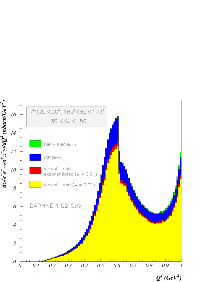
Figure 3: Initial state radiation in the process $e^{+}e^{-}\rightarrow\pi^{+}\pi^{-}\gamma$ at the Born (blue) and NLO level for $\sqrt{s}=1.02$ GeV. Virtual plus soft contributions are considered with a soft cutoff equal to $w=0.01$ at fixed order (yellow) and exponentiated (red). The final state radiation contribution (including interference with ISR) is also shown (green). The cuts are: $7^{o}<\theta_{\gamma}<20^{o}$ or $160^{o}<\theta_{\gamma}<173^{o}$, $30^{o}<\theta_{\pi}<150^{o}$ and the energy of the observed photon $E_{\gamma}>0.02$ GeV.

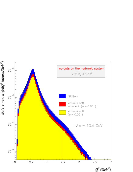
Figure 4: Initial state radiation in the process $e^{+}e^{-}\rightarrow\pi^{+}\pi^{-}\gamma$ at the Born (blue) and NLO level for $\sqrt{s}=10.6$ GeV. Virtual plus soft contributions are considered with a soft cutoff equal to $w=0.001$ at fixed order (yellow) and exponentiated (red). The cuts are: $7^{o}<\theta_{\gamma}<173^{o}$ and the energy of the observed photon $E_{\gamma}>0.02$ GeV.

The leptonic tensor can be cast, from eq.(12) and appendix A, into the form:

$$L^{\mu\nu} =L_{0}^{\mu\nu}\bigg{\{}1+\frac{\alpha}{\pi}\bigg{[}-\log(4w^{2})[1+\log(m^{2})]$$

$$-\frac{3}{2}\log(m^{2})-2+\frac{\pi^{2}}{3}\bigg{]}\bigg{\}}+C^{\mu\nu}~{},$$ (17)

where the expected soft and collinear behaviour is manifest. The first term, $\log(4w^{2})[1+\log(m^{2})]$, coming from the emission of soft photons, gives a large contribution which eventually could spoil the improvement expected from a NLO analysis. The soft cutoff $w$ should be small enough to justify the soft photon approximation. On the other hand, a very small value of $w$ would result in a meaningless negative cross-section. To overcome this difficulty, the contribution of a second hard photon, with energy $E_{\gamma}>w\sqrt{s}$, should be added inpreparation , thus canceling the $w$-dependence. However, one may also limit the analysis to configurations where the additional radiated photon is required to be soft, by constraining the invariant mass of the hadron + photon system. For small $w$ the following exponentiation can be used:

$$1-\frac{\alpha}{\pi}\log(4w^{2})[1+\log(m^{2})]\rightarrow(2w)^{-\frac{2\alpha}{\pi}[1+\log(m^{2})]}~{}.$$ (18)

This accounts for the leading soft logarithms to all orders in perturbation theory exponentiation and vanishes in the limit $w\rightarrow 0$, as expected.

Another contribution which can be rather large and was not considered up to now, is the insertion of vacuum polarization corrections to the virtual photon line in figure 1. Its inclusion does not affect the other features of our calculation. It introduces a correction which is proportional to the Born leptonic tensor and can be reabsorbed in the choice of a running coupling constant. In order to take into account also the higher orders, a factor $1/(1-\delta_{VP})$ where $\delta_{VP}$ is the vacuum polarization contribution can be included. In the present version of this program, this factor has been dropped for simplicity.

Motivated by these considerations, the following improved leptonic tensor can be defined:

$$L^{\mu\nu} =\frac{(2w)^{-\frac{2\alpha}{\pi}[1+\log(m^{2})]}}{1-\delta_{VP}}$$ (19)

$$\times \bigg{[}L_{0}^{\mu\nu}\bigg{\{}1+\frac{\alpha}{\pi}\bigg{[}-\frac{3}{2}\log(m^{2})-2+\frac{\pi^{2}}{3}\bigg{]}\bigg{\}}+C^{\mu\nu}\bigg{]}~{}.$$

4 Monte Carlo simulation

A Monte Carlo generator has been built. It simulates the process $e^{+}e^{-}\rightarrow\pi^{+}\pi^{-}\gamma$ where the photon is emitted from the initial state, with a large angle with respect to the beam direction. It is based on EVA Binner:1999bt and includes the NLO corrections described in the previous sections . The program is built in a modular way such that the simulation of other exclusive hadronic channels can be easily included while keeping the factorization of the initial state QED corrections. Configurations with an additional hard photon are not yet included. Hence the generator can only be used to describe configurations where the invariant mass of the hadronic system plus the tagged photon is close to the total energy of the collision, $M(\gamma+hadrons)>(1-w)\sqrt{s}$. A generator which includes also emission of two hard photons will be presented in a subsequent publication.

In figure 3, the differential distribution in the invariant mass of the hadronic system is shown for the process $e^{+}e^{-}\rightarrow\pi^{+}\pi^{-}\gamma$ at DAPHNE energies, $\sqrt{s}=1.02$ GeV. In principle, initial and final state radiation (FSR) would be required for the complete simulation of the process. However, the cuts: pions in the central region, $30^{o}<\theta_{\pi}<150^{o}$, and photons close to the beam and well separated from the pions, $7^{o}<\theta_{\gamma}<20^{o}$ or $160^{o}<\theta_{\gamma}<173^{o}$, select configurations dominated by initial state radiation Binner:1999bt ; Melnikov:2000gs . For comparison, the contribution of the final state radiation at Born level is also shown. The corrections to the Born approximation reach up to $20\%$ for a soft cutoff of $w=0.01$ if the fixed order expression (17) is used, or $17\%$ if the exponentiation of the soft cutoff, eq.(18), is applied.

At B-factories, $\sqrt{s}=10.6$ GeV, the situation is slightly different. Because of the higher center of mass energy, the hadronic system and the real photon are mainly produced back to back. The FSR is therefore already suppressed without imposing additional kinematical cuts on the hadronic system. For these high energies one might in addition include photons emitted also at larger angles. From the analysis of EVA Binner:1999bt one finds that the events are always dominated by ISR – a consequence of the strong form factor suppression of FSR at high energies and large angles between pions and photons. Figure 4 shows the differential distribution in the invariant mass of the hadronic system at $\sqrt{s}=10.6$ GeV for photons in the region $7^{o}<\theta_{\gamma}<173^{o}$ and no constraints to the hadronic system. The FSR amounts to less than $10^{-3}$ and is not shown. The NLO corrections are again dominated by the value of the soft photon cutoff.

5 Leading log resummation

From the results of the previous section, it is clear that the fixed order correction is dominated by the value of the soft photon cutoff $w$. Even if the exponentiation is applied, which accounts for the leading soft logarithms to all orders in perturbation theory, the situation does not improve much. The addition of the contribution of a second hard photon would cancel the strong $w$-dependence, however, large logarithms of collinear origin, $L=\log(s/m_{e}^{2})$, would remain. Because these large logarithms will show up in all orders of perturbation theory, resummation techniques have been developed which are constructed to include the dominant higher order terms. The method of structure functions structure ; Berends:1988ab accounts well for these corrections. It takes into account all the leading logarithmic corrections $\cal{O}$$(\alpha L)$, coming from virtual, soft, and hard photon contributions to all orders in perturbation theory.

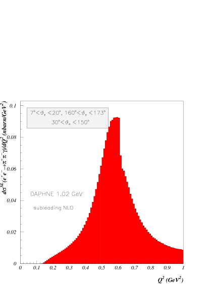
Figure 5: Subleading NLO contribution to initial state radiation in the process $e^{+}e^{-}\rightarrow\pi^{+}\pi^{-}\gamma$. Same cuts as in figure 3.

In Binner:1999bt these effects were considered in the simulation of the process $e^{+}e^{-}\rightarrow\pi^{+}\pi^{-}\gamma$. The formulas of Caffo:1997yy were used which include terms up to order $\alpha^{2}L^{2}$. A minimal invariant mass of the $\pi^{+}\pi^{-}\gamma$ system was required in order to reduce the kinematic distorsion of the events due to the collinear initial state radiation. For a sufficiently tight cut this corresponds to the situation discussed in the present paper. For a minimal invariant mass of the $\pi^{+}\pi^{-}\gamma$ system of $0.9$ GeV², a negative $6\%$ correction to the Born approximation was found.

Subleading effects, which correspond to the $C^{\mu\nu}$ terms of our leptonic tensor in eq.(17), are not taken into account within this approximation. In figure 5, the contribution of these subleading terms to the differential distribution of figure 3 is shown. They amount to $0.6\%$ of the Born approximation close to the $\rho$-resonance, where the rate is maximal, and to $1\%$ for small values of $Q^{2}$, where, however, the cross section rate is small. Similar values are found for higher center of mass energies. The matching of the resummed result, through the structure function technique, with the fixed order result is under study inpreparation .

6 Conclusions

ISR at high luminosity $e^{+}e^{-}$ colliders ($\phi$ and $B$-factories) is an alternative to the direct measurement of $\sigma(e^{+}e^{-}\rightarrow hadrons)$ giving access to a wide range of energies, from threshold to the center of mass energy of the collider. The NLO QED correction to ISR, in the form of a leptonic tensor, has been calculated and included in a Monte Carlo generator, which was compared with EVA Binner:1999bt for the $\pi^{+}\pi^{-}$ exclusive channel. The modular structure of the calculation, independent of the final state hadronic system, is such that other hadronic channels or improved parametrizations of the hadronic current can be easily included.

From our results it is clear that the fixed order correction is dominated by the value of the soft photon cutoff $w$. Only the contribution of a second hard photon inpreparation would cancel this strong $w$-dependence. But even if this contribution is added, large logarithms of collinear origin, $L=\log(s/m_{e}^{2})$, would still remain. Furthermore, they will show up in all orders of perturbation theory. A consistent way to resum such leading log terms together with subleading effects is also under consideration inpreparation .

Appendix A Tensor coefficients

In this appendix, we collect our results for the scalar coefficients of the leptonic tensor (12) at the NLO arising from virtual and soft photon contributions. Our expressions are valid in the limit of small electron mass.

For the coefficient proportional to $g^{\mu\nu}$, we get

$$a_{00}^{(1)} =a_{00}^{(0)}\bigg{[}-\log(4w^{2})[1+\log(m^{2})]$$

$$-\frac{3}{2}\log(\frac{m^{2}}{q^{2}})-2+\frac{\pi^{2}}{3}\bigg{]}$$

$$-\frac{q^{2}(1-q^{2})}{2}-y_{1}y_{2}-\bigg{[}q^{2}+\frac{2y_{1}y_{2}}{1-q^{2}}\bigg{]}\log(q^{2})$$

$$+\frac{y_{1}}{2}\bigg{[}4-y_{1}-\frac{3(1+q^{2})}{1-y_{2}}\bigg{]}\log(\frac{y_{1}}{q^{2}})$$

$$+\frac{y_{2}}{2}\bigg{[}4-y_{2}-\frac{3(1+q^{2})}{1-y_{1}}\bigg{]}\log(\frac{y_{2}}{q^{2}})$$

$$-\bigg{[}1+(1-y_{2})^{2}+\frac{y_{1}q^{2}}{y_{2}}\bigg{]}L(y_{1})$$

$$-\bigg{[}1+(1-y_{1})^{2}+\frac{y_{2}q^{2}}{y_{1}}\bigg{]}L(y_{2})~{},$$ (20)

with

$$L(y_{i})=Li_{2}(\frac{-y_{i}}{q^{2}})-Li_{2}(1-\frac{1}{q^{2}})+\log(q^{2}+y_{i})\log(\frac{y_{i}}{q^{2}})~{},$$

where $Li_{2}$ is the Spence or dilogarithm function and $y_{i}$, $q^{2}$ and $m^{2}$ have been defined in eq.(5). The quantity $w$ denotes the dimensionless value of the soft photon energy cutoff: $E_{\gamma}<w\sqrt{s}$. The coefficient in front of the tensor structure $p_{1}^{\mu}p_{1}^{\nu}$, is given by

$$a_{11}^{(1)} =a_{11}^{(0)}\bigg{[}-\log(4w^{2})[1+\log(m^{2})]$$ (21)

$$-\frac{3}{2}\log(\frac{m^{2}}{q^{2}})-2+\frac{\pi^{2}}{3}\bigg{]}$$

$$+(1+q^{2})^{2}\left(\frac{1}{1-y_{1}}-\frac{1}{1-q^{2}}\right)-\frac{4(1-y_{2})y_{1}}{1-q^{2}}$$

$$-\frac{2q^{2}}{1-q^{2}}\bigg{[}(1-y_{2})\left(\frac{1}{y_{2}}+\frac{q^{2}}{y_{1}}+\frac{2y_{1}}{1-q^{2}}\right)$$

$$+\frac{2q^{2}}{1-q^{2}}\bigg{]}\log(q^{2})-q^{2}\bigg{[}1+\frac{2}{y_{2}}\bigg{]}\log(\frac{y_{1}}{q^{2}})$$

$$-q^{2}\bigg{[}\frac{(2-3y_{1})(1-y_{2})^{2}}{y_{1}(1-y_{1})^{2}}\bigg{]}\log(\frac{y_{2}}{q^{2}})$$

$$-2q^{2}\bigg{[}1+\frac{1}{y_{2}^{2}}\bigg{]}L(y_{1})-2q^{2}\bigg{[}3+\frac{2q^{2}}{y_{1}}+\frac{q^{4}}{y_{1}^{2}}\bigg{]}L(y_{2})~{},$$

that in front of $p_{2}^{\mu}p_{2}^{\nu}$ can be obtained by symmetric considerations, exchanging the positron with the electron momenta

$$a_{22}^{(1)}=a_{11}^{(1)}(y_{1}\leftrightarrow y_{2})~{}.$$ (22)

For the symmetric tensor structure ($p_{1}^{\mu}p_{2}^{\nu}+p_{2}^{\mu}p_{1}^{\nu}$), we get

$$a_{12}^{(1)} =\frac{q^{2}}{1-y_{1}}+\frac{q^{2}}{1-y_{2}}-\frac{4q^{2}+(y_{1}-y_{2})^{2}}{1-q^{2}}$$ (23)

$$-2q^{2}\bigg{[}\frac{q^{2}}{y_{1}y_{2}}+\frac{1+q^{2}-2y_{1}y_{2}}{(1-q^{2})^{2}}\bigg{]}\log(q^{2})$$

$$-\frac{2q^{2}}{1-y_{2}}\bigg{[}1-y_{1}+\frac{q^{2}}{y_{2}}-\frac{q^{2}}{2(1-y_{2})}\bigg{]}\log(\frac{y_{1}}{q^{2}})$$

$$-\frac{2q^{2}}{1-y_{1}}\bigg{[}1-y_{2}+\frac{q^{2}}{y_{1}}-\frac{q^{2}}{2(1-y_{1})}\bigg{]}\log(\frac{y_{2}}{q^{2}})$$

$$-2q^{2}\bigg{[}1+\frac{q^{2}}{y_{2}}+\frac{q^{2}}{y_{2}^{2}}\bigg{]}L(y_{1})-2q^{2}\bigg{[}1+\frac{q^{2}}{y_{1}}+\frac{q^{2}}{y_{1}^{2}}\bigg{]}L(y_{2})~{}.$$

Finally, the antisymmetric coefficient $a_{-1}$, accompanying ($p_{1}^{\mu}p_{2}^{\nu}-p_{2}^{\mu}p_{1}^{\nu}$), reads

$$a_{-1}^{(1)} =q^{2}\bigg{[}\frac{\log(m^{2}y_{2})}{y_{1}}+\frac{1-q^{2}}{1-y_{1}}+\frac{q^{2}}{(1-y_{1})^{2}}\bigg{]}$$

$$-(y_{1}\leftrightarrow y_{2})~{}.$$ (24)

Appendix B Loop integrals and soft photon contribution

The Passarino-Veltman procedure Passarino:1979jh allows to reduce the calculation of any one-loop amplitude to the evaluation of a few scalar one-loop integrals. In this appendix, we collect the scalar one-loop integrals needed for our calculation and give their expression in the limit of small electron mass. Ultraviolet (UV) and infrared (IR) divergences appear in the one-loop calculation. Dimensional regularization in $D=4-2\varepsilon$ dimensions is used to regularize both kind of divergences. The UV divergences are renormalized using the on-shell renormalization scheme. The soft photon contribution to the leptonic tensor cancels the remaining IR divergences.

A few two-, three-, and four-point scalar one-loop integrals enter our calculation. Expression for the two-point scalar integrals are simple and well known. The general three-point scalar one-loop integral is defined by

$$C_{0}(p_{a}^{2},(p_{a}-p_{b})^{2},p_{b}^{2},m_{1}^{2},m_{2}^{2},m_{3}^{2})=-i16\pi^{2}\mu^{4-D}$$

$$\times\int\frac{d^{D}k}{(2\pi)^{D}}\frac{1}{[k^{2}-m_{1}^{2}][(k-p_{a})^{2}-m_{2}^{2}][(k-p_{b})^{2}-m_{3}^{2}]}~{}.$$ (25)

Four different three-point scalar one-loop integrals are needed

$$C01=C_{0}((p_{i}-k_{1})^{2},0,m_{e}^{2},0,m_{e}^{2},m_{e}^{2})~{},$$

$$C02=C_{0}(m_{e}^{2},s,m_{e}^{2},0,m_{e}^{2},m_{e}^{2})~{},$$

$$C03=C_{0}((p_{i}-k_{1})^{2},Q^{2},m_{e}^{2},0,m_{e}^{2},m_{e}^{2})~{},$$

$$C04=C_{0}(Q^{2},s,0,m_{e}^{2},m_{e}^{2},m_{e}^{2})~{},$$ (26)

$i=1,2$, and one scalar box

$$D0=-i16\pi^{2}\mu^{4-D}\int\frac{d^{D}k}{(2\pi)^{D}}$$ (27)

$$\times\frac{1}{k^{2}[(k+p_{i})^{2}-m_{e}^{2}][(k+p_{i}-k_{1})^{2}-m_{e}^{2}][(k-p_{j})^{2}-m_{e}^{2}]}~{},$$

with $j\neq i$.

In the limit of vanishing electron mass: $m^{2}\ll s,Q^{2},y_{i}$, the following results are obtained:

$$C01=\frac{s^{-1}}{y_{i}}\bigg{[}-\frac{1}{2}\log^{2}\frac{m^{2}}{y_{i}}-\frac{\pi^{2}}{3}\bigg{]}~{},$$

$$C02=s^{-1}\bigg{[}\log(m^{2})\Delta-\frac{\log^{2}(m^{2})}{2}-\frac{2\pi^{2}}{3}+i\pi\Delta\bigg{]}~{},$$

$$C03=\frac{s^{-1}}{q^{2}+y_{i}}\bigg{[}\log(m^{2})\log(\frac{y_{i}}{q^{2}})-2\log(q^{2}+y_{i})\log(\frac{y_{i}}{q^{2}})+$$

$$\quad\frac{\log^{2}(y_{i})}{2}-\frac{\log^{2}(q^{2})}{2}-2Li_{2}(\frac{-y_{i}}{q^{2}})-\frac{7\pi^{2}}{6}+i\pi\log(\frac{y_{i}}{q^{2}})\bigg{]}~{},$$

$$C04=\frac{s^{-1}}{1-q^{2}}\bigg{[}\log(m^{2})-\frac{\log(q^{2})}{2}+i\pi\bigg{]}\log(q^{2})~{},$$

$$D0=\frac{s^{-2}}{y_{i}}\bigg{[}-\log(m^{2})\Delta+2\log(m^{2})\log(\frac{y_{i}}{q^{2}})-2Li_{2}(1-\frac{1}{q^{2}})$$

$$\quad-\frac{5\pi^{2}}{6}-i\pi\bigg{(}\Delta-\log(m^{2})-2\log(\frac{y_{i}}{q^{2}})\bigg{)}\bigg{]}~{},$$ (28)

where

$$\Delta=\frac{(4\pi)^{\varepsilon}}{\varepsilon\;\Gamma(1-\varepsilon)}\left(\frac{\mu^{2}}{s}\right)^{\varepsilon}~{}.$$ (29)

They can be compared, for instance, with the one-loop integrals quoted in Berends:1986yy where a fake photon mass $\lambda$ was used to regularize the IR divergences. The identification $\Delta\leftrightarrow\log(\lambda^{2}/s)$ allows to pass from one scheme to the other.

B.1 Initial state soft photon emission

The contribution to the leptonic tensor of a soft photon with momentum $k$ and energy $E<w\sqrt{s}$, with $w\ll 1$, reads

$$L_{soft}^{\mu\nu} =-4e^{2}\frac{\mu^{4-D}}{2(2\pi)^{D-1}}\int_{0}^{w\sqrt{s}}E^{D-3}dEd\Omega$$

$$\times\left(\frac{p_{1}}{2p_{1}\cdot k}-\frac{p_{2}}{2p_{2}\cdot k}\right)^{2}L_{0}^{\mu\nu}~{}.$$ (30)

Integrated in the soft photon phase space Rodrigo:1999gv and in the limit of small electron mass, we get

$$L_{soft}^{\mu\nu}=\frac{\alpha}{\pi}\bigg{\{} \left[\Delta-\log(4w^{2})\right]\left[1+\log(m^{2})\right]$$

$$-\frac{\log^{2}(m^{2})}{2}-\log(m^{2})-\frac{\pi^{2}}{3}\bigg{\}}L_{0}^{\mu\nu}~{}.$$ (31)

After UV renormalization, the renormalized one-loop matrix elements $\tilde{M}_{i}$ of the diagrams in figure 2, which contribute at the NLO to the leptonic tensor through their interference with the Born diagrams, give the following IR contribution

$$L_{IR}^{\mu\nu} =\sum_{i=1,4}(\overline{\tilde{M}_{i}^{\mu}M_{0}^{\nu+}+M_{0}^{\mu}\tilde{M}_{i}^{\nu+}})\big{|}_{\varepsilon}=$$

$$=-\frac{\alpha}{\pi}\Delta\left[\log(m^{2})+1\right]L_{0}^{\mu\nu}~{}.$$ (32)

Summing up eq.(31) and eq.(32), a finite result is found.

References

• (1) H. N. Brown et al. [Muon g-2 Collaboration], Phys. Rev. Lett.  86 (2001) 2227 [hep-ex/0102017].
• (2) V. W. Hughes and T. Kinoshita, Rev. Mod. Phys. 71 (1999) S133.
• (3) W. J. Marciano and B. L. Roberts, [hep-ph/0105056]. F. Jegerlehner, [hep-ph/0104304]. M. Davier and A. Höcker, Phys. Lett. B 435 (1998) 427 [hep-ph/9805470]. S. Eidelman and F. Jegerlehner, Z. Phys. C 67 (1995) 585 [hep-ph/9502298]. K. Adel and F. J. Yndurain, [hep-ph/9509378].
• (4) H. Burkhardt and B. Pietrzyk, LAPP-EXP-2001-03. A. D. Martin, J. Outhwaite and M. G. Ryskin, [hep-ph/0012231]; Phys. Lett. B 492 (2000) 69 [hep-ph/0008078]. J. Erler, Phys. Rev. D 59 (1999) 054008 [hep-ph/9803453]. J. H. Kühn and M. Steinhauser, Phys. Lett. B 437 (1998) 425 [hep-ph/9802241].
• (5) S. Binner, J. H. Kühn and K. Melnikov, Phys. Lett.  B459 (1999) 279 [hep-ph/9902399].
• (6) K. Melnikov, F. Nguyen, B. Valeriani and G. Venanzoni, Phys. Lett.  B477 (2000) 114 [hep-ph/0001064].
• (7) S. Spagnolo, Eur. Phys. J. C 6 (1999) 637.
• (8) V. A. Khoze, M. I. Konchatnij, N. P. Merenkov, G. Pancheri, L. Trentadue and O. N. Shekhovzova, Eur. Phys. J. C 18 (2001) 481 [hep-ph/0003313].
• (9) A. Denig, talk given at Physics at Intermediate Energies Workshop, SLAC, April 2001. M. Adinolfi et al. [KLOE Collaboration], [hep-ex/0006036].
• (10) Solodov, talk given at Physics at Intermediate Energies Workshop, SLAC, April 2001.
• (11) J. H. Kühn and A. Santamaria, Z. Phys. C 48 (1990) 445.
• (12) H. Czyz and J. H. Kuhn, Eur. Phys. J. C 18 (2001) 497 [hep-ph/0008262].
• (13) H. Czyż, J. H. Kühn and G. Rodrigo, in preparation.
• (14) R. Mertig, M. Böhm and A. Denner, Comput. Phys. Commun. 64 (1991) 345.
• (15) G. Passarino and M. Veltman, Nucl. Phys. B 160 (1979) 151.
• (16) F. A. Berends, G. J. Burgers and W. L. van Neerven, Phys. Lett.  B177 (1986) 191.
• (17) D. R. Yennie, S. C. Frautschi and H. Suura, Annals Phys. 13 (1961) 379. F. Bloch and A. Nordsieck, Phys. Rev. 52 (1937) 54.
• (18) E. A. Kuraev and V. S. Fadin, Sov. J. Nucl. Phys. 41 (1985) 466. G. Altarelli and G. Martinelli, in Physics at LEP, CERN-Yellow Report 86-06, eds. J. Ellis and R. Peccei (CERN, Geneva, February 1986). O. Nicrosini and L. Trentadue, Phys. Lett. B196 (1987) 551.
• (19) F. A. Berends, W. L. van Neerven and G. J. Burgers, Nucl. Phys.  B297 (1988) 429; Erratum Nucl. Phys.  B304 (1988) 921.
• (20) M. Caffo, H. Czyż and E. Remiddi, Nuovo Cim.  A110 (1997) 515 [hep-ph/9704443]; Phys. Lett.  B327 (1994) 369.
• (21) G. Rodrigo, A. Santamaria and M. Bilenky, J. Phys. G25 (1999) 1593 [hep-ph/9703360].