Resonant Amplification of Electroweak Baryogenesis at Preheating

Abstract

We explore viable scenarios for parametric resonant amplification of electroweak (EW) gauge fields and Chern-Simons number during preheating, leading to baryogenesis at the electroweak (EW) scale. In this class of scenarios time-dependent classical EW gauge fields, essentially spatially-homogeneous on the horizon scales, carry Chern-Simons number which can be amplified by parametric resonance up to magnitudes at which unsuppressed topological transitions in the Higgs sector become possible. Baryon number non-conservation associated with the gauge sector and the highly non-equilibrium nature of preheating allow for efficient baryogenesis. The requisite large CP violation can arise either from the time-dependence of a slowly varying Higgs field (spontaneous baryogenesis), or from a resonant amplification of CP violation induced in the gauge sector through loops. We identify several CP violating operators in the Standard Model and its minimal extensions that can facilitate efficient baryogenesis at preheating, and show how to overcome would-be exponential suppression of baryogenesis associated with tunneling barriers.

1 Introduction

Parametric resonance coupling of the oscillating inflaton to Standard Model fields [1] offers new dynamical mechanisms for various early-universe phenomena. One interesting scenario [2, 3, 4] adjusts inflaton parameters so that reheating does not heat the universe to a temperature above the EW cross-over temperature $T_{c}$. This means that sphaleron transitions are frozen out and that B+L created before reheating will not be washed out.

The early attempts [6, 7] to create B+L solely through Standard Model effects suffered from the fact that if the only source of CP violation is in the CKM matrix, it would lead to far too small a value of B+L, and from the need for a first-order EW phase transition to drive out-of-equilibrium effects. This first-order transition seems to be ruled out by current lower limits on the Higgs mass of around 110 GeV. So it might appear that EW baryogenesis is unattractive. However, with the suggestion of EW preheating and the accompanying parametric resonances, it has become interesting to look at EW baryogenesis in a different way.

This was done in a recent paper [8], where two of us showed that EW parametric resonance, with the Higgs field oscillating because of its coupling to the oscillating inflaton, could amplify CP-violating seed values of the EW gauge potential in an $ansatz$ where this gauge potential was spatially-homogeneous (out to the horizon) but time-dependent. The CP violation was manifested as a homogeneous classical “condensate” of Chern-Simons number or equivalently of B+L (through the EW anomaly). The scenario of [8] had several shortcomings:

1. CP violation only occurred because of CP-violating initial values for the gauge potential, not because of any explicit CP violation in the gauge equations of motion.

2. The Higgs field oscillations were considered as given, so that no (classical) back-reaction of the gauge fields on the Higgs field was considered.

3. No plausible scenario was suggested for the permanent conversion of Chern-Simons number to actual baryons and leptons; once parametric resonance driving ended, it would be possible for the homogeneous Chern-Simons condensate to dissipate. Actual formation of baryons and leptons requires the development of spatial inhomogeneities, rather similar to sphalerons; one might term this process sphalerization.

In the present work we extend the considerations of [8] to deal, at least partially, with these three shortcomings.

First, we introduce explicit CP violation in the EW gauge plus Higgs equations of motion. This CP violation comes from coupling of CP-violating effects to the EW gauge fields through loops, typically quark loops. We explore two cases; in one, there is out-of-equilibrium strong CP violation as evidenced by an $\eta^{\prime}$ field slowly (on EW time scales) rolling in a standard QCD potential with zero $\theta$ angle (so that there is no strong CP violation when the $\eta^{\prime}$ field is in equilibrium). In the other, we invoke spontaneously-broken CP in multi-Higgs models [10], again, out of equilibrium. Note that it is not easy to rule out the CP-violating operators we use by present-day experimental results on CP violation, since in our scenario the CP-violating effects are far from their equilibrium values.

Second, we study the combined gauge field-Higgs classical equations, extending the previous $ansatz$ to include a spatially-homogeneous time-dependent Higgs field. The classical backreaction of the gauge potential on the Higgs field can drive the Higgs field into oscillating through zero VEV rather than staying near a broken-symmetry minimum. This is important for sphalerization.

Third, in the final section of the paper we make some remarks about the dynamics of sphalerization. This is a truly difficult dynamical problem, requiring extensive numerical investigation, and we barely scratch the surface here. Aside from brute-force computation, not attempted here, there are several avenues to explore for guidance, including simple effective-temperature arguments previously used in connection with EW preheating[1, 3, 4]; numerical studies of the 1+1-dimensional Abelian Higgs model[3, 4, 11]; and approximate but useful tools for an analysis based on tools developed for understanding the possibility of B+L violation in high-energy two-particle collisions (see, e.g., [12]). A major obstacle to the analysis is that mere production of Chern-Simons number is not enough to produce baryons; the Chern-Simons number must be converted into baryons through the medium of formation of Higgs winding number $N_{\rm wind}$. Using simple topological arguments, we construct a model for the energy profile of the system which illustrates the issues involved. With the simplification of using an effective temperature we estimate baryoproduction for an arbitrary time dependence of the topological transition rate and show how wash-out—fermionic backreaction leading to dissipation of the newly-created baryons and leptons—can be taken into account. Finally we attempt an alternative to effective-temperature considerations by extending some approximate techniques used long ago to examine the possibility of B+L violation in two-particle collisions.

The upshot of these considerations is that there are at least two possibilities for conversion of Chern-Simons number to baryons which do not suffer from the exponential suppression of tunneling. In the first, various effects (such as gauge backreaction on the Higgs field) may cause the Higgs VEV $v(t)$ to oscillate through zero during or immediately after preheating, allowing unsuppressed transitions (the sphaleron mass $M_{S}\sim v/g$ vanishes). In the second, formation of spatial structures on various scales may allow for baryon formation to proceed at energies above barrier heights even if $v$ is near its usual broken-symmetry value. In this case, there is a relation between the size of the structure, the energy of the structure, and the Chern-Simons density, which we explore with a relatively crude but qualitatively satisfactory model of the topological charge barrier factor as a function of energy and size. We argue that as various spatial scales arise and grow during preheating and the Chern-Simons condensate becomes inhomogeneous, it is possible to have conversion of Chern-Simons number to actual baryons (and leptons, which we ignore in this paper) which is not only unsuppressed with regard to topological charge tunneling, but is also not exponentially suppressed by poor overlap between initial and final states. This is an important point. About a decade ago, it was suggested that EW collisions of two particles yielding an $N$-particle final state at energies $E\geq M_{S}$ large enough to overcome the barrier height and with $N\sim 4\pi/g^{2}$, could lead to unsuppressed B+L production (see, e.g., [12] for a contemporaneous collection of papers on the subject). But others (including Banks et al [12] and Cornwall [12, 13]) pointed out that the poor overlap between the initial and final states led to exponential suppression anyhow, with a barrier which was a finite fraction of the canonical ’t Hooft barrier. The suppression mechanism had actually been proposed earlier by Drukier and Nussinov [14] to show that production of solitons such as the sphaleron in two-particle collisions was exponentially suppressed.

In the present case, the initial state for baryogenesis is not a two-particle plane-wave state, but a Chern-Simons condensate which is largely homogeneous and on which various spatial ripples are growing, as suggested in [8]; when the gauge potential grows to be of order $m/g$, the spatial growth rate is of order $m$. We show that this sort of condensate can have good overlap with baryonic final states (as connected via the EW anomaly) at certain spatial scales under the same circumstances (generally high enough energy) where the topological barrier is gone. These spatial scales, to no one’s surprise, are around $m^{-1}$ at energies near the sphaleron mass. Of course, if the Higgs VEV $v$ is rather small, the corresponding spatial scale grows larger and the energy scale grows smaller. We show that if this second mechanism to avoid suppression is to work when $m$ is near its vacuum value, the original spatially-homogeneous Chern-Simons condensate must have a density of order $10^{-2}-10^{-3}$ units of topological charge in a volume $m^{-3}$. Such values are indeed reached in numerical simulations (this paper and Ref. [8]).

We cannot, with these crude approaches, begin to quantify the number of baryons produced. All we can say is that the number of baryons is essentially linear in the strength of the CP-violating operators we discuss, and that we are not aware of any experimental limits which would lead to strengths too small to produce the observed number of baryons, provided that the baryogenesis process is not exponentially suppressed and that further baryon washout at reheating is not strong. Given the results of this paper, the unexplored rate-limiting step for baryogenesis is the growth of perturbations at various spatial scales.

For some simple versions of the models we study it is possible to do some approximate analysis of growth of Chern-Simons number in the spatially-homogeneous phase. Generally we find that adding explicit CP violation to the gauge equations of motion leads, as expected, to secular (that is, not oscillating with the inflaton or Higgs) CP-violating terms in the gauge potential and Chern-Simons density. If the explicit CP violation is correlated on super-Hubble scales, as might be expected following inflation and which we will assume for this paper, the secular average will also be correlated on super-Hubble scales even though initial values of the gauge potentials might be random from one Hubble domain to the next. Without explicit CP violation in the equations of motion, CP violation can only come from CP-violating initial values of the EW gauge fields; if (as mentioned in [8]) these are random from one Hubble volume to the next and on the average CP-symmetric, the baryon number averaged over the whole universe will be zero and fluctuations will be too small by the usual factor of $1/\sqrt{N}$, where $N$ is the number of Hubble volumes. (Of course, CP-violating effects before preheating can be correlated on super-Hubble scales, so that there can be a secular average with no explicit CP violation in the equations of motion.) We offer one model, somewhat resembling a Brownian ratchet [15], in which the secular Chern-Simons average depends not only on the sign of the explicit CP violation (assumed to have super-Hubble correlations) but also on the sign of initial conditions, which we could assume as random and uncorrelated. Nonetheless, this model leads to a sort of secular Chern-Simons average, since resonant growth can occur only for one sign of initial-condition parameters; otherwise, there is damping. In this model, however, the secular average itself wanders slowly on a long time scale and consequently is somewhat inefficient. We also offer other models in which the secular Chern-Simons sign depends only on the sign of the explicit CP-violating term in the equation of motion; these lead to a Chern-Simons condensate of unique sign across the universe.

We will give a few examples of numerical simulations, making no attempt to cover the possible range of initial conditions and models. The examples are chosen to illustrate strong resonance and hence strong amplification of CP violation; in effect, this means that EW gauge potentials become of order the vacuum Higgs VEV $v$ and the Chern-Simons density grows to order $m^{3}/8\pi^{2}$. In strong resonance these final values are essentially independent of the initial values; only the time needed to reach the final values changes with initial conditions. With no resonance there is little or no amplification, and (in our scenarios) far too few baryons would be produced. We are in no position to say what “final” values of the Chern-Simons condensate are needed to produce today’s B+L values, since our understanding of the conversion of Chern-Simons number to B+L in this very non-equilibrium process is still quite primitive.

Our general conclusions are that while there are still many unknowns, involving both parameters of CP-violating physics and unsolved dynamics, we know of nothing which would rule out generation of the observed number of baryons in the universe today in this EW preheating scenario.

Other points of view [1, 2, 3, 16] have been expressed concerning the mechanisms at work during EW preheating, including the invocation of approximate thermalization of long-wavelength gauge boson modes at an effective temperature much larger than the eventual reheat temperature, so that EW symmetry is effectively restored, and more or less genuine thermalization of shorter wavelengths. Without further numerical simulations it is impossible for us to say how such ideas compare to what we suggest here, which is based on ultimate conversion of a spatially-homogeneous Chern-Simons condensate [8] to a condensate more resembling sphalerons.

There is one numerical lattice simulation [17] of the full d=3+1 Higgs-gauge system which does not show any secular growth of Chern-Simons number, which instead decays to near zero. For technical reasons these authors did not include CP-violating terms in the gauge equations of motion. As we show here, such terms are important to establish a long-term Chern-Simons condensate, which may undergo sphalerization and conversion to baryons.

2 Spontaneous baryogenesis at preheating

Biasing the baryon asymmetry through an effective chemical potential can be achieved in a model with two Higgs doublets in what is known as spontaneous baryogenesis. Cohen, Kaplan, and Nelson [7, 9] proposed that the effective T-reversal asymmetry may come from a time dependence in the solution for the Higgs field. Their scenario used the variation of the Higgs field inside a wall of a bubble formed in a first-order phase transition. A similar effect can occur at preheating uniformly in space, on the horizon scales. We will discuss this scenario on an example of a two-doublet model.

The Higgs potential in a general model with two doublets, $H_{1}$ and $H_{2}$, has a form

$$V(H_{1},H_{2}) = \lambda_{1}(H_{1}^{\dagger}H_{1}-v_{1}^{2})^{2}$$ (1)

$$+ \lambda_{2}(H_{2}^{\dagger}H_{2}-v_{2}^{2})^{2}$$

$$+ \lambda_{3}[(H_{1}^{\dagger}H_{1}-v_{1}^{2})+(H_{2}^{\dagger}H_{2}-v_{2}^{2})]^{2}$$

$$+ \lambda_{4}[(H_{1}^{\dagger}H_{1})(H_{2}^{\dagger}H_{2})-(H_{1}^{\dagger}H_{2})(H_{2}^{\dagger}H_{1})]$$

$$+ \lambda_{5}[{\rm Re}(H_{1}^{\dagger}H_{2})-v_{1}v_{2}\cos\xi]^{2}$$

$$+ \lambda_{6}[{\rm Im}(H_{1}^{\dagger}H_{2})-v_{1}v_{2}\sin\xi]^{2}$$

At finite temperature, all $\lambda_{k}$ and $v_{i}$ receive thermal corrections and depend on the temperature.

During preheating the Higgs fields move along some classical trajectory

$$H_{i}=\rho_{i}(t)e^{i\theta_{i}(t)}$$ (2)

that satisfies the equations of motion

$$\ddot{\theta_{i}}+3h\dot{\theta_{i}}+\frac{\dot{\rho_{i}}}{\rho_{i}}+\rho_{i}^{-1}\frac{\partial V}{\partial\theta_{i}} = 0,$$

$$\ddot{\rho_{i}}+3h\dot{\rho_{i}}-\dot{\theta_{i}}^{2}{\rho_{i}}+\frac{\partial V}{\partial\rho_{i}} = 0,$$ (3)

where $h$ is the Hubble constant. The term $(\partial V/\partial\theta_{i})$ is non-vanishing as long as there is a mixing between the Higgs bosons; this term is periodic in $\theta_{i}$.

In the course of reheating, fermions are created and a thermal equilibrium is achieved at some temperature $T_{R}<100$GeV, low enough to prevent any sphaleron transitions. The Higgs fields change from their zero-temperature values at the end of inflation to some temperature-dependent VEV:

$${\rm at}\ T = 0,\ \ \rho_{i}=v_{i};$$ (4)

$${\rm at}\ T = T_{{}_{R}},\ \ \rho_{i}=v_{i}(T_{{}_{R}}).$$ (5)

At the same time, the phase $\theta$ also changes:

$$\theta(0) \equiv \theta_{1}(0)-\theta_{2}(0)=\xi,$$ (6)

$$\theta(T_{{}_{R}}) \equiv \theta_{1}(T_{{}_{R}})-\theta_{2}(T_{{}_{R}})=\xi(T_{{}_{R}}).$$ (7)

The time derivative of $\theta$ serves as a chemical potential for the baryon number [9, 19] because of an effective coupling

$$(\partial_{0}\theta)j^{0}_{{}_{Y}}$$ (8)

that appears in the Lagrangian after the time-dependent phase is eliminated from the Yukawa couplings. Here $j^{\mu}_{{}_{Y}}=m_{t}\bar{\psi}\gamma^{\mu}\psi+...$ is the fermionic current.

If the gauge fields grow in resonance as described in Ref. [8], but the Higgs fields are out of resonance, the $\dot{\rho}/\rho$ term in equation (3) can be neglected. The equation allows for a slowly varying solution $\bar{\theta}(t)$ that interpolates between $\theta=\xi$ and $\theta=\xi(T_{{}_{R}})$. Since the Chern-Simon number violating processes in the gauge sector are very rapid on the time scale of thermalization, the fermions produced during reheating will have time to equilibrate to the minimum of free energy when a thermal distribution is ultimately achieved. The effective chemical potential $\mu_{{}_{B}}$ is proportional to $\dot{\theta}$, and the equilibrium value of baryon asymmetry is

$$n_{{}_{B}}\sim\langle\dot{\theta}\rangle\left(\frac{y_{t}v(T_{{}_{R}})}{T_{{}_{R}}}\right)^{2}T_{{}_{R}}^{2}\sim\frac{\xi}{t_{{}_{R}}}\left(\frac{y_{t}v(T_{{}_{R}})}{T_{{}_{R}}}\right)^{2}T_{{}_{R}}^{2}\sim 10^{-10}\ T_{{}_{R}}^{3}\ \left(\frac{10^{-5}t_{{}_{H}}}{t_{{}_{R}}}\right),$$ (9)

where $t_{{}_{R}}$ is the time of reheating and $t_{{}_{H}}$ is the Hubble time at the electroweak scale, $y_{t}$ is the top Yukawa coupling, and $v(T)$ is the Higgs VEV. For $T_{{}_{R}}\leq 70$GeV, there is no wash-out of the baryon number by thermal sphalerons. The required baryon asymmetry, $10^{-10}$, can be achieved in this scenario if the reheat time is $10^{-5}$ the Hubble time. The reheat time is usually much shorter than the Hubble time, and the requisite ratio $10^{-5}$ can be achieved in a realistic model.

The difference with the scenario proposed by Cohen, Kaplan and Nelson [9] is that in our case CP violation occurs homogeneously in space, as opposed to in a bubble wall. In addition, the final prediction for baryon asymmetry in the CKN scenario was very far from the equilibrium value (9) because the sphaleron rate was slow on the time scales associated with the growth of the bubble. In our case, $\theta$ changes slowly in time while the baryon number non-conservation is rapid. This allows a slow adiabatic adjustment of the baryon number to that which minimizes the free energy.

3 CP-Violating Operators and Coupling to the EW Gauge Fields

In this section we describe some models of parametric-resonance-enhanced CP and B+L violation which are (at least immediately following inflation) spatially-homogeneous over each Hubble volume, but not fully-correlated over super-horizon regions. These models evade, in various ways, the usual problem that B+L generation in any one Hubble volume is completely uncorrelated to neighboring Hubble volumes. In these models there is one or more feature which is totally-correlated (because of inflation), typically the inflaton VEV or the time-dependent part of Higgs VEVs as driven by coupling to the inflaton. But other features, such as initial values of other fields, may be totally uncorrelated from one Hubble volume to the next. Unlike the earlier study [8] explicit CP violation is built in to the gauge-field equations of motion rather than just into initial values; this CP bias can overcome randomness due to initial values and to stochastic behavior of the solutions to the equations of motion.

The CP-violating terms come from various higher-dimensional operators which can be generated from strong CP violation or from multi-Higgs models showing spontaneous CP violation [10]. The coupling strengths of such CP-violating operators need not be small, since in the early universe strong CP violation can be very much out of equilibrium. Generally the higher-dimension operators come from fermion loops; in the kinematic situation of the present paper, there is no way for a purely bosonic system of gauge fields, inflaton, and Higgs to lead to CP-violating terms in the gauge equations of motion. We will only consider $local$ CP-violating terms, which would be appropriate at the beginning of pre-heating when the universe is very cold; in principle, modifications of locality can occur when the time dependence of various quantities begins to probe the fermion loops carrying the CP violation. We will not consider that case here.

There are two generic CP-violating operators which we will consider. The first is of the form

$$\kappa F{\rm\,Tr\,}G_{\mu\nu}\tilde{G}^{\mu\nu}$$ (10)

where $\tilde{G}$ is the dual field strength for the EW $SU(2)$ group, $F(x)$ is a (possibly composite) gauge-singlet field and $\kappa$ a coupling strength with dimensions of mass to some negative power (depending on $F$). As usual, integration by parts of equation (10) shows that the action can contribute to the gauge-field equations of motion only if $F$ has a non-trivial dependence on $x$; we will seek for this dependence in out-of-equilibrium oscillations of the inflaton or other fields. We note that coupling of the form (10) as a source for topological number density has been considered in a model with a cosmological pseudoscalar field coupled to hypercharge [20].

Another possibility is:

$$\kappa^{\prime}F{\rm\,Tr\,}G_{\mu\nu}G_{\nu\alpha}\tilde{G}_{\alpha\mu}.$$ (11)

In this case, it is not required that there be any extra field $F(x)$, since the operator in equation (11) is not a total divergence. Nonetheless we include it, since there are terms in the gauge-field part of (11) which are total divergences and which could be important.

When the action constructed from operators of the type (10, 11) is added to the EW gauge action and the Higgs equation of motion is added, the dynamics studied in [8] are modified. We discuss the new equations of motion following some brief remarks on the physics behind the operators in (10). As for the higher-dimension operator in equation (11), it is to be expected at some level whenever the lower-dimension operator in equation (10) appears.

4 CP-Violating Physics

The CP-violating physics we are concerned with may come from out-of-equilibrium strong CP violation, from CP violation in the Higgs sector (with two or more Higgs fields), or from other causes. (Note that CKM phase effects are not strong enough to drive CP violation in the Standard Model.) We will discuss the first two explicitly.

4.1 A model with strong CP violation

Consider the CP-violating operator of equation (10), which has a typical axionic form, although we do not associate the field $F$ with an axion. We assume that previous physics associated with earlier times has left a universe which has substantial strong CP violation in the QCD sector. As a prototypical example, consider the $\eta^{\prime}$ field, which is coupled to the QCD quark anomaly and to the gluonic topological charge density. This coupling to quarks is of the usual form

$$M_{q}\bar{q}\exp[\frac{i\gamma_{5}\eta^{\prime}}{F_{\eta^{\prime}}}]q$$ (12)

(with suitable but irrelevant normalization of $F_{\eta^{\prime}}$), showing that $\eta^{\prime}/F_{\eta^{\prime}}$ is an angle with period $2\pi$. The potential energy of the $\eta^{\prime}$ field comes from (12) and from coupling to gluons; the latter must reflect the Witten-Veneziano [21] relation and other requirements related to the $\theta$-angle dependence of QCD. The result is the standard form:

$$V(\eta^{\prime})={\rm min}_{j}\;\varepsilon_{\rm QCD}\cos[\frac{1}{N_{c}}(\theta+2\pi j+\eta^{\prime}/F_{\eta^{\prime}})]$$ (13)

where $j=0,1,2$, $N_{c}=3$ is the number of colors, $\theta$ is the usual QCD vacuum angle, $\varepsilon_{\rm QCD}$ is the QCD gluonic vacuum energy density ($\varepsilon_{\rm QCD}\simeq g_{s}^{2}\langle{\rm\,Tr\,}G_{s}^{2}\rangle$ in terms of the strong coupling $g_{s}$ and field strength $G_{s}$; note that $\varepsilon_{\rm QCD}<0$ with our conventions using antihermitean gauge fields). To be specific, let us suppose that the vacuum angle is zero and that $\eta^{\prime}/F_{\eta^{\prime}}$ is small enough so that we need consider only the $j=0$ sector explicitly. Now suppose that through the operation of some early-universe physics the field $\eta^{\prime}$ deviates substantially from its equilibrium value of zero. Furthermore, this deviation, because of inflation, is (roughly) the same across the entire universe. Just as the inflaton does, the $\eta^{\prime}$ field will begin to roll toward its equilibrium value (at which point strong CP violation is absent or small) on a QCD time scale $\sim GeV^{-1}$, a time scale long compared to all other time scales in the problem. The $\eta^{\prime}$ field couples to the EW fields $G_{\mu\nu}$ through, e.g., quark loops, yielding an effective coupling

$$\kappa_{\rm QCD}\eta^{\prime}\frac{1}{32\pi^{2}}{\rm\,Tr\,}G_{\mu\nu}\tilde{G}^{\mu\nu}.$$ (14)

It is straightforward to check that $\kappa_{\rm QCD}^{-1}$ is of order a QCD mass $M$ of 1 GeV or so. The coupling to the EW potential $\phi$ requires an integration by parts, yielding a term in the action $\sim\kappa_{\rm QCD}\dot{\eta^{\prime}}\phi^{3}$, where $\phi$ is a constituent of the EW gauge potential (see equation (21) below).

It might also happen that the field $F$ coupled to the topological charge density oscillates at the inflaton rate, because of Higgs couplings to the inflaton. For example, with the notation $H$ for an electroweak Higgs field doublet, some unspecified physics may lead to an action of the type of equation (10)

$$\kappa\frac{g^{2}}{16\pi^{2}}\int d^{4}xH^{{\dagger}}H{\rm\,Tr\,}G_{\mu\nu}\tilde{G}^{\mu\nu}$$ (15)

where the field $F=H^{{\dagger}}H$ oscillates at inflaton rate scales because the Higgs field is coupled to the inflaton.

4.2 CP violation in a multi-Higgs sector

Since we are in no position to be very specific about CP violation in the early universe, we will illustrate the concept by using a model (T. D. Lee in [10]) which cannot account for all CP violation observed in the $K-\bar{K}$ system, but which can nevertheless represent an additional source of CP violation in the early universe. In this model there are two Higgs doublets $H_{1},H_{2}$, and the potential is chosen so that even though all couplings are real, the $H_{2}$ VEV is complex and of the form

$$\langle H_{2}\rangle=\left(\begin{array}[]{c}0\\ v_{2}e^{i\theta}\end{array}\right)$$ (16)

with real positive $v_{2}$. The phase angle $\theta$ arises from terms in the Higgs potential of the form

$$V=H^{{\dagger}}_{1}H_{2}(DH^{{\dagger}}_{1}H_{2}+EH^{{\dagger}}_{1}H_{1})+H.c.+\dots$$ (17)

which can be rewritten to show terms involving $\cos\theta$:

$$V=2Dv_{1}^{2}v_{2}^{2}(\cos\theta+\frac{Ev_{1}}{4Dv_{2}})^{2}+\dots$$ (18)

Recall that the essence of EW-scale pre-heating is coupling of the inflaton to the EW Higgs fields. In this case, we invoke (for no deep physics reasons) a coupling of the form

$$G\sigma^{2}H^{{\dagger}}_{1}H_{2}+H.c.\sim v_{1}v_{2}\sigma^{2}\cos\theta,$$ (19)

assuming for simplicity that the coupling $G$ is real. Once pre-heating sets in and the inflaton $\sigma(t)$ begins oscillating, the angle $\theta$ also begins to oscillate.

The CP violation is coupled through $SU(2)$ fermions to the EW gauge fields, and one readily checks that the lowest-order fermion loop graph gives rise to a coupling of the type in equation (10) which is proportional to $v_{1}v_{2}\sin\theta$. The oscillations of $\theta$ then give rise to a non-trivial coupling to the EW gauge field $\phi$.

5 CP-Violating Equations of Motion

There are several possibilities for CP-violating terms in the equations of motion, depending, for example, on whether the field $F(x)$ in equation (10) oscillates at the inflaton oscillation frequency, or at a much lower frequency. Before writing down these terms we set the notation by giving the Standard Model action for the gauge and Higgs fields, including a coupling of the Higgs field to the inflaton field $\sigma$ (but not writing other inflaton terms):

$$S=\int d^{4}x\left[\frac{1}{2g^{2}}{\rm\,Tr\,}G_{\mu\nu}G^{\mu\nu}+D_{\mu}H^{{\dagger}}D^{\mu}H-\lambda(H^{{\dagger}}H-\frac{1}{2}v^{2})^{2}-G^{2}\sigma^{2}H^{{\dagger}}H\right]$$ (20)

We use, as before [8], the following ansatz for the EW gauge potential, which is $g$ times the canonical potential and is written in antihermitean matrix form (so that $D_{\mu}=\partial_{\mu}+A_{\mu}$):

$$A_{0}=0;\;\;A_{j}=(\frac{\tau_{j}}{2i})\phi(t),$$ (21)

with corresponding electric and magnetic fields:

$$E_{j}\equiv G_{0j}=(\frac{\tau_{j}}{2i})\dot{\phi};\;\;B_{j}\equiv\frac{1}{2}\epsilon_{jkl}G_{kl}=(\frac{\tau_{j}}{2i})\phi^{2}.$$ (22)

For the Higgs field $H$ we use the Standard Model form

$$\langle H\rangle=\left(\begin{array}[]{c}0\\ v(t)/\sqrt{2}\end{array}\right)$$ (23)

Evidently the topological charge density goes like $\dot{\phi}\phi^{2}$, which is, as it must be, a total time derivative. The topological charge density is the time derivative of the Chern-Simons density $n_{{}_{\rm CS}}$:

$$n_{{}_{\rm CS}}=\frac{\phi^{3}}{8\pi^{2}}.$$ (24)

The gauge and Higgs equations will be written in non-dimensional form, where the time variable is replaced by $mt$, the gauge field $\phi$ is replaced by $\phi/m$, and the Higgs field $v$ is replaced by $v/v_{0}$. Here $m=v_{0}g/2$ is the vacuum W-boson mass in terms of the standard Higgs VEV $v_{0}$. The resulting equations are:

$$\ddot{\phi}+2\phi^{3}+v^{2}\phi+[{\rm CP-violating\;term}]=0$$ (25)

and

$$\ddot{v}+\frac{3}{4}\phi^{2}v+(\frac{M_{H}^{2}}{2m^{2}})v(v^{2}-1)+(\frac{G^{2}\sigma^{2}}{m^{2}})v=0.$$ (26)

where $M_{H}=v_{0}\sqrt{2\lambda}$ is the Higgs mass. An important property of equation (26) is that if large (order one) values of $\phi$ are reached by resonant amplification, the Higgs potential is strongly modified and $v$ can approach the symmetry-restoring value of zero.

There are, as discussed above, several possibilities for the CP-violating term. In these equations we will assume that the inflaton is oscillating sinusoidally at a physical frequency $\omega$, corresponding to a dimensionless frequency $r/2$:

$$\sigma=\sigma_{0}\cos(\frac{rt}{2});\;\;\omega=\frac{rm}{2}.$$ (27)

Previously instead of using the Higgs equation of motion (26) the Higgs potential was set to zero, on the grounds that inflation stops, preheating starts, and the EW sector begins to undergo spontaneous symmetry breaking when the inflaton field reaches the critical value $\sigma_{c}$:

$$\sigma_{c}=\frac{M_{H}}{G\sqrt{2}}.$$ (28)

This led to

$$v^{2}=1+2\epsilon+2\epsilon\cos rt;\;\;\epsilon\equiv\frac{-\sigma_{0}^{2}}{4\sigma_{c}^{2}}.$$ (29)

Under the assumption that $\epsilon$ is small, so that it can be ignored compared to unity in the constant term in (29), the gauge equation of motion became [8]:

$$\ddot{\phi}+2\phi^{3}+(1+\epsilon\cos rt)\phi=0.$$ (30)

Note that there is no CP violation in equation (30), since for any solution $\phi(t)$ there is another solution $-\phi(t)$. CP violation can only come from initial values which favor one sign or the other of the CP-odd field $\phi$. The modifications we address in the next subsection add terms even in $\phi$ to the equations of motion, which therefore will have a built-in CP bias. And when we come to numerical analysis in Sec. 5, we will use equations (25, 26) instead of the simplified form $1+\epsilon\cos rt$ in equation (30) above.

5.1 CP violation at the inflaton oscillation rate

Before studying the complications of the combined Higgs-gauge equations (25, 26) which can really only be handled numerically, we will look at adding CP-violating terms to the simplified gauge dynamics of equation (30). This allows a certain amount of approximate analysis, similar to that used in the Mathieu equation, to be done.

Using the Higgs dependence on time as shown in (29) and integrating by parts in the action of equation (15) gives rise to an action of the form $\int\phi^{3}\sin\omega t$. We add the appropriate contribution to equation (30) leading to the modified (and explicitly CP-violating) equation:

$$\ddot{\phi}+2\phi^{3}+\delta\phi^{2}\sin rt+(1+\epsilon\cos rt)\phi=0.$$ (31)

In this equation the parameter $\delta$ is proportional to $\kappa\epsilon\omega v_{0}^{2}$. Note that if $\phi(t)$ is the solution to (31), then $-\phi(t)$ is the solution to this equation when $\delta$ is changed in sign.

Without the $\delta\phi^{2}$ term the equation of motion is essentially a Lamé equation, as discussed in [8]. But with this term added we know of no way of reducing the equation of motion to explicitly-soluble form. The major feature of the modified equation can be found by a standard Mathieu-like analysis, assuming that $\phi$ has the form

$$\phi(t)=a(t)\cos(rt/2)+b(t)\sin(rt/2)+c(t)$$ (32)

and assuming that $a,b,c$ vary slowly on the time scale of oscillations. The new feature here is the presence of the secular term $c$, which is unnecessary when the $\delta\phi^{2}$ term is missing in (31). By ignoring all terms oscillating faster than the half-frequency $r/2$ one then finds:

$$0 = r\dot{a}+b[\frac{r^{2}}{4}+\frac{\epsilon}{2}-1-\frac{3}{2}(a^{2}+b^{2})]-\delta ac;$$ (33)

$$0 = -r\dot{b}+a[\frac{r^{2}}{4}-\frac{\epsilon}{2}-1-\frac{3}{2}(a^{2}+b^{2})]-\delta bc;$$

$$c = \frac{-\delta ab}{1+3(a^{2}+b^{2})}.$$

Note that since both $\delta$ and $c$ are proportional to the parametric-resonance parameter $\epsilon$, the new (last terms on the right-hand side of (33)) contributions are of order $\epsilon^{2}$. The formal analysis is done in powers of $\epsilon$, which we therefore assume to be small. Then in (33) the equations for $a$ and $b$ are, to order $\epsilon$, the same as without the $\delta$ term, and the secular term $c$ is driven by the unperturbed values of $a,b$. These show standard Mathieu behavior of the form $\exp\mu t$ with

$$\mu=\pm\frac{1}{2r}[\epsilon^{2}-(r^{2}-4)]^{1/2}$$ (34)

(where we ignore temporarily non-linearities in the equations). Since $\epsilon$ is small, the value of $r$ must be nearly two for $\mu$ to be real and resonant amplification to take place, which is to say that $\mu$ scales linearly with $\epsilon$.

In studying the original equation with no $\delta$ term but retaining the cubic non-linearity [8], it was shown that the quantity $a^{2}+b^{2}$ obeyed a certain equation which revealed the conditions under which growth rather than damping (negative $\mu$) occurred. With the $\delta$ term added, this equation is:

$$\frac{d}{dt}(a^{2}+b^{2})=\frac{-2\epsilon ab}{r}-\frac{2\delta^{2}ab(a^{2}-b^{2})}{1+3(a^{2}+b^{2})}.$$ (35)

The second term on the right of (35) is of higher order and can be neglected, and then the conclusion is the same as before: Growth is only possibly if $ab$ is positive (for negative $\epsilon$); otherwise there is damping. (When $a,b$ are small, their growth leads to growth of the secular term $c$, at twice the rate of growth of $a$ or $b$; see (33).)

Writing

$$a=A\cos\Psi,b=-A\sin\Psi$$ (36)

with positive amplitude $A$, Ref. [8] showed from (35) that

$$A=A_{0}\exp\int_{0}^{t}dt^{\prime}\frac{\epsilon}{2r}\sin 2\Psi(t^{\prime})$$ (37)

with an accompanying equation for the angle $\Psi$ showing that it varied on the $\epsilon$ rate scale, that is, slowly. Eventually $\Psi$ becomes large enough so that the product $ab$ changes sign and growth turns into damping, or vice versa.

What is happening to the Chern-Simons number in this model? The Chern-Simons number density is just $\phi^{3}/8\pi^{2}$, and in the case where the CP-violating term proportional to $\delta$ is absent, as is the secular term $c$, this quantity is purely oscillatory and has no appreciable long-term average or preferred sign. But things are different with $\delta\neq 0$; the secular average of the Chern-Simons density is:

$$\langle\frac{\phi^{3}}{8\pi^{2}}\rangle=\frac{3}{16\pi^{2}}cA^{2}$$ (38)

Note that the sign of the Chern-Simons density is controlled by the sign of the secular term $c$. Under the usual assumption that the inflaton (and therefore the Higgs) field is correlated across the entire universe, because of inflation, the sign of $\delta$ is also correlated across the universe and by (33) the sign of $c$ depends on the sign of the product $ab$, which may differ in each Hubble volume. But by equation (35) growth only occurs when this product is positive (since $\epsilon$ is negative), even though $a,b$ may separately be random in each Hubble volume. Of course, only those Hubble volumes where growth actually takes place have appreciable Chern-Simons density and in each of these volumes the sign of the Chern-Simons density is the same. There are Hubble volumes with Chern-Simons density of the opposite sign, but in them there is no growth and this density is small. The result is that at least for a while the entire universe has an average Chern-Simons density of fixed sign, the same in each Hubble volume, even though the initial values of gauge potentials may be random in each Hubble volume.

Numerical simulations discussed below show that on time scales of order $\epsilon^{-1}$ the secular average can change sign, since on such time scales the product $ab$ can also change sign. This may lead to relatively small Chern-Simons condensate values even in strong resonance.

We cannot yet say how small or large this condensate value must be, in order to reproduce the observed value of B+L, or of the baryon-photon ratio. The smallness of the baryon-photon ratio must come, in our models, from a combination of the smallness of CP-violating parameters (such as occur in Higgs potentials), dynamical effects during pre-heating such as mentioned above, and sphaleron washout after pre-heating.

5.2 Equations of motion with strong CP violation

Since the $\eta^{\prime}$ field potential in equation (13) is determined by QCD parameters it is rolling very slowly on EW time scales and we can replace the time derivative of $\eta^{\prime}$ by a term of order $M\eta^{\prime}$, where $M$ is a typical QCD mass, and ultimately (after rescaling time and the EW potential $\phi$ as before) come to another CP-violating $\phi$ equation of the form:

$$\ddot{\phi}+2\phi^{3}+\delta^{\prime}\phi^{2}+(1+\epsilon\cos rt)\phi=0.$$ (39)

Here the parameter $\delta^{\prime}$ is of order $M/m$, the ratio of QCD and EW scales, or perhaps $10^{-2}$.

As before, we must add a secular term $c$ to the usual Mathieu ansatz of equation (32). Equations (33) are changed; the equations of motion for $a,b$ are the same as with no CP violation (that is, set $\delta=0$ in the first two equations of (33)) while the equation for $c$ becomes:

$$c=\frac{-\delta^{\prime}(a^{2}+b^{2})}{2[1+3(a^{2}+b^{2})]}.$$ (40)

Provided that (as we have already assumed) $\delta^{\prime}$ is roughly the same in all Hubble volumes, so is the sign of $c$, and so the Chern-Simons numbers in all Hubble volumes add with the same sign.

5.3 Higher-derivative CP violation

We briefly consider here the consequences of adding the higher-derivative CP violation of equation (11). It is readily checked that this term yields actions $\sim\int F(\dot{\phi}^{3})$ and $\sim F\phi^{4}\dot{\phi}$; the latter is integrated by parts to $\sim\dot{H}\phi^{5}$. So to the original equations of motion we must add terms of the form

$$\dot{F}\phi^{4};\;\;-3(\dot{F}\dot{\phi}^{2}+2F\dot{\phi}\ddot{\phi}).$$ (41)

These can, as discussed in connection with the numerical studies reported below, have dramatic effects because of the appearance of derivatives of $\phi$.

6 Numerical studies

The range of parameter space is vast, and cannot be covered in depth here. We give several examples illustrating most of the effects discussed above. In these examples, we will use the following values of parameters unless otherwise specified:

1. Gauge initial values: $\phi(0)=0.01;\;\dot{\phi}(0)=0.01$

2. Higgs initial values: $v(0)=0.5;\;\dot{v}(0)=0.5$

3. Epsilon parameter $\epsilon=0.5$

4. $M_{H}^{2}/2m^{2}=1.5$ (corresponding to a Higgs mass of about 140 GeV)

5. Resonance parameter $r=2.2$

Other parameters will be specified as needed. Note that for this standard set of parameters the Higgs field is far from equilibrium; below we give numerics for initial values starting rather close to equilibrium.

6.1 Sinusoidal CP violation with gauge backreaction

Gauge backreaction is described by equations (25, 26), to which we will add appropriate CP-violating terms. One of the most important features of this gauge backreaction is that it can help facilitate rapid Higgs transition through $v=0$, which removes the sphaleron barrier and makes baryons from Chern-Simons number. The equations to be studied numerically here are (26) plus a gauge equation with a sinusoidal CP-violating term:

$$\ddot{\phi}+2\phi^{3}+v^{2}\phi+\delta\phi^{2}\sin rt=0.$$ (42)

The initial conditions are as given at the beginning of this Section, except that $\dot{\phi}(0)=-0.01$; also, $\delta=0.51$. This value of $\delta$ is not necessarily realistic, but in general CP-violating quantities scale linearly in $\delta$. The change of sign is done in order to get on the positive-$\epsilon$ growth curve of the parametric-resonance instability of the simplified version of the gauge equation of motion, given in equation (31). Fig. 1 shows the results for $\phi$, $v$, Chern-Simons density $n_{{}_{\rm CS}}$, and the running average $\langle n_{{}_{\rm CS}}\rangle$ of the Chern-Simons density, defined as:

$$\langle n_{{}_{\rm CS}}\rangle=\frac{1}{t}\int_{0}^{t}dt^{\prime}n_{{}_{\rm CS}}(t^{\prime}).$$ (43)

There is no particular physical significance to the running average, but it is more convenient to display than the time-integrated Chern-Simons number, which covers too large a range to be displayed legibly. More to the point is a simple time integral of $n_{{}_{\rm CS}}$ such as emerges from the dynamics, as in equation (60) below; this is 600 times the running average at the end of the time period simulated.

One notes that in the present model the running average $\langle n_{{}_{\rm CS}}\rangle$ itself changes sign from time to time on a long time scale, as would be expected from the analysis of Sec. 5.1. So this model is not a particularly efficient way of generating B+L even in strong resonance. On the other hand, just how large a long-term Chern-Simons condensate needs to be to generate the observed B+L is not known, so this may or may not be a drawback.

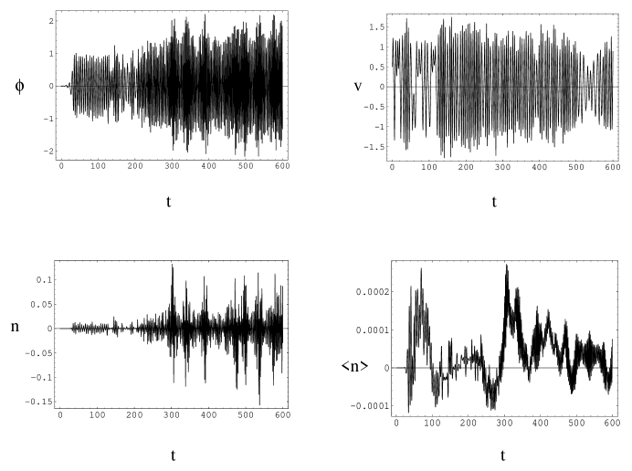
Figure 1: These figures show the behavior of the dimensionless gauge potential $\phi$, Higgs VEV $v$, Chern-Simons density $n\equiv n_{{}_{\rm CS}}$, and the running average of the Chern-Simons density $\langle n\rangle\equiv\langle n_{{}_{\rm CS}}\rangle$ for the conditions of Sec. 6.1.

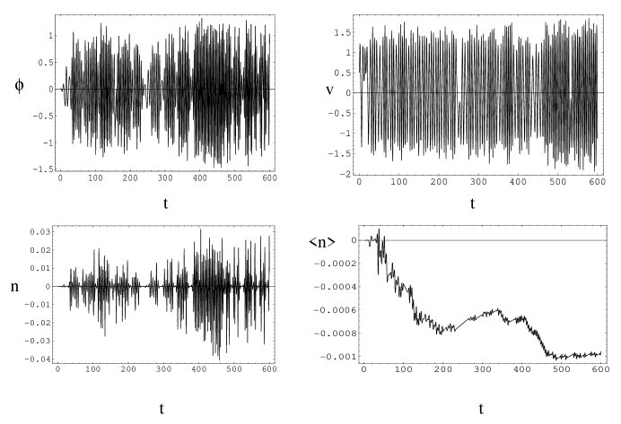
Figure 2: These figures show the behavior of $\phi,\;v,\;n_{{}_{\rm CS}},$ and $\langle n_{{}_{\rm CS}}\rangle$ for the conditions of Sec. 6.2 with $v(0)=\dot{v}(0)$=0.5.

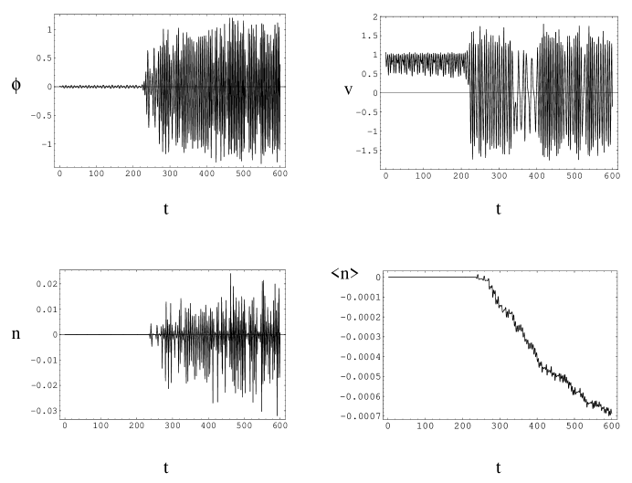
Figure 3: These figures show the behavior of $\phi,\;v,\;n_{{}_{\rm CS}},\;$ and $\langle n_{{}_{\rm CS}}\rangle$ for the conditions of Sec. 6.2, with $v(0)$=1.06, $\dot{v}(0)$=0.1.

6.2 Constant CP violation with gauge backreaction

In the present example we modify equation (25) by adding a quadratic CP-violating term with constant coefficient, as discussed in Sec. 5.2:

$$\ddot{\phi}+2\phi^{3}+v^{2}\phi+w\phi^{2}=0$$ (44)

We will take $w=0.5$ for the numerical example. This is unrealistically large, but it makes it easier to see what is happening. Generally speaking, the long-term average Chern-Simons density is proportional to $w$; for example, as in the simplified analysis (with no gauge back-reaction) leading to equations (38),(40) which gives:

$$\langle n_{{}_{\rm CS}}\rangle=-{1\over{16\pi^{2}}}w\langle\phi^{2}\rangle$$ (45)

or $\langle n_{{}_{\rm CS}}\rangle\sim-0.0008$ for Figs. 2 and 3.

Fig. 2 shows the time history of $\phi,\;v$, the Chern-Simons density $n_{{}_{\rm CS}}$, and the running average $\langle n_{{}_{\rm CS}}\rangle$ for initial Higgs values which are far from equilibrium. The integrated Chern-Simons number is of order 0.1 for a CP-violating strength of order unity, and so might be of order $10^{-4}$ for more realistic CP-violating amplitudes $w$ of order $10^{-3}$. This leaves room for inefficiencies in generating B+L from Chern-Simons number, washout of B+L, and other dynamical effects to reduce the baryon number to its actual level of perhaps $10^{-10}$. And, of course, there is no reason to believe that the numerical parameters we use here apply to the real early universe. Experience with running many simulations of the type in Fig. 2 shows that the initial values of Higgs and gauge fields are not so important, and that final values of the running Chern-Simons average for unit-strength CP violation range from about $10^{-3}$ (somewhat smaller than the maximum expected, which is of order $1/8\pi^{2}$), to the non-resonant value of $\phi(0)^{3}/8\pi^{2}$ which is of order $10^{-8}$ for our initial conditions. Of course, these values would be reduced further by the strength of the CP-violating term, which is not small in our simulations.

In the examples so far, the Higgs field has been far from equilibrium initially and so it swings through the origin frequently. The next example, also for a constant CP-violating term, shows the importance of gauge backreaction in causing the Higgs field to oscillate through zero. For this example we choose Higgs initial values $v(0)=1.06,\;\dot{v}(0)=0.1$ with all other parameters as for Fig. 2. The results are shown in Fig. 3. Because the Higgs field is near equilibrium, it stays for a while near unity, and the gauge field appears to be trivially small. Actually $\phi$ is slowly growing and finally becomes large around a time of 200. Fast growth of $\phi$ towards order unity values begins to send the Higgs field into wild oscillation, accompanied by growth of the Chern-Simons average value. We will see later that having the Higgs field go through the origin may be important for creating baryons from the Chern-Simons condensate.

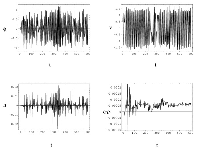
Figure 4: These figures show $\phi,\;v,\;n_{{}_{\rm CS}},$ and $\langle n_{{}_{\rm CS}}\rangle$ for the conditions of Sec. 6.3.

6.3 Higher-derivative CP violation

Adding terms such as those in equation (41) can and sometimes does lead to singularities in finite time because of the higher derivatives. We show one case where the singularity does not develop before dimensionless time 600. The equations to be solved numerically are the Higgs equation (26) and:

$$\ddot{\phi}+2\phi^{3}+v^{2}\phi+w(\alpha\dot{\phi}^{2}+\dot{\phi}\ddot{\phi})=0.$$ (46)

The coefficients $w,\alpha$ are -0.2 and 0.1 respectively. If $w$ gets even a little larger in magnitude (say, $w=-0.21$) a singularity seems to develop, although we have not explored this phenomenon in any detail. Fig. 4 shows the results. The $\dot{\phi}^{2}$ term in (46) is always of one sign and leads to secular CP violation; if only the $\dot{\phi}\ddot{\phi}$ term were kept, the running-average CP violation slowly wanders from one sign to the other.

7 From Chern-Simons Number to Baryons

In this section we comment on some very difficult questions: How is the homogeneous condensate of Chern-Simons number, equivalent to a B+L condensate, turned into actual baryons and leptons, which are localized states? What fraction of the condensate is turned into baryons and leptons? How does the winding number of the Higgs field enter in? We are in no position to give definitive answers; all these questions are still under active investigation.

Let us begin with a comment concerning washout of baryons and leptons after reheating. The attractive feature of EW preheating is that the temperature after full reheating is rather smaller than the EW cross-over temperature $T_{c}$, so that baryons and leptons created during preheating are not completely washed out (the sphaleron transition rate $\sim\exp(-M_{S}/T)$ is very small because the sphaleron mass $M_{S}$ is large compared to the temperature). We will assume that this mechanism protects baryons, once produced, from washout during reheating. Nonetheless, there can be washout during preheating, and we will have to discuss that.

Our discussion will invoke insights derived from numerical and analytical work on these issues in the 1+1-dimensional Abelian Higgs model; from simple arguments based on effective temperature; and on approximations to an analysis based on modifications of earlier work on B+L violation in two-particle collisions (where B+L violation is still extremely small because of the poor overlap of states, even though there may be no tunneling barrier).

A real baryon is a spatially-localized state, so the transformation to baryons requires quasi-localized states resembling (but not necessarily identical to) sphalerons; these states involve not only the gauge fields but also Higgs fields, which carry a winding number $N_{\rm wind}$ of their own. In the ansatz we have used so far the Higgs field has no winding number.

Presumably a major influence on the dynamics of spatial localization is the instability of the gauge-Higgs equations to growth of spatial ripples, as alluded to in [8]. We will not discuss this mechanism here, which is non-linear and time-dependent (so it may be amplified by parametric resonance).

7.1 Dependence of energy on topological quantum numbers

In the presence of a Chern-Simons condensate it is energetically favorable to shift the winding number of the Higgs field $N_{\rm wind}$ in the direction of Chern-Simons number. One way to see this is to note that the energy $E=\int d^{3}x\varepsilon$ depends on both $N_{{}_{\rm CS}}$ and $N_{\rm wind}$. In the homogeneous $ansatz$ used so far the energy, with terms in $\phi^{2}$ and $\phi^{4}$, grows monotonically with $n_{{}_{\rm CS}}$ since $n_{{}_{\rm CS}}\sim\phi^{3}$. The Higgs winding number $N_{\rm wind}$ is zero (see equation (23)). Now the energy of a state with finite values of $N_{\rm wind},\;N_{{}_{\rm CS}}$ is, under a large gauge transformation with Chern-Simons number $-N_{\rm wind}$, equivalent to one with zero Higgs winding:

$$E(N_{{}_{\rm CS}},N_{\rm wind})=E(N_{{}_{\rm CS}}-N_{\rm wind},N_{\rm wind}=0)$$ (47)

By the above remarks the energy with $N_{\rm wind}=0$ has its minimum at $N_{{}_{\rm CS}}-N_{\rm wind}=0$.

More explicitly, once the system has become a condensate of more or less localized objects, these are described by a large gauge transformation at spatial infinity:

$$A_{\mu}\rightarrow U\partial_{\mu}U^{-1},$$ (48)

$$H(x)\rightarrow\frac{1}{\sqrt{2}}U\left(\begin{array}[]{c}0\\ v_{0}\end{array}\right).$$ (49)

The same gauge transformation $U$ appears in both the gauge potential and in the Higgs field in order that the Higgs contribution $\int|D\phi|^{2}$ to the action be finite in infinite volume. Evidently these localized states have lower energy than a homogeneous condensate which, so to speak, fills in the volume between the localized states.

The vacuum states with $N_{{}_{\rm CS}}=N_{\rm wind}$ are minima on the energy landscape, so $E(N_{{}_{\rm CS}},N_{\rm wind})$ is zero along the line $N_{{}_{\rm CS}}=N_{\rm wind}$. Any transitions proceeding toward this line are energetically favorable. For example, beginning from the homogeneous $ansatz$ state with large positive $N_{{}_{\rm CS}}$ but zero $N_{\rm wind}$, it is favorable to $decrease$ $N_{{}_{\rm CS}}$ and $increase$ $N_{\rm wind}$. Of course, it is also energetically favorable to decrease $N_{{}_{\rm CS}}$ toward zero with no change in $N_{\rm wind}$, but then no baryons will be produced; B+L will rise and fall in lockstep with $N_{{}_{\rm CS}}$, according to the usual anomaly relation, yielding no baryons at the end. So among the changes which decrease $N_{{}_{\rm CS}}$ there is a competition between those which increase $N_{\rm wind}$ and those which do not change $N_{\rm wind}$.

We illustrate these statements in Figs. 5, 6, 7, 8. Fig. 5 is drawn assuming that the gauge boson mass (and a posteriori the sphaleron mass) are somewhere near their conventional values, so that there is a sphaleron barrier hindering topological charge change as indicated by the corrugations on the figure. However, as we have seen in the numerical studies, it is possible for this barrier to vanish as the Higgs VEV passes through zero. Fig. 6 is a view from above of the energy profile plot of Fig. 5. In Fig. 6 the filled circles along the $N_{{}_{\rm CS}}=N_{\rm wind}$ line indicate states of zero energy (with $N_{\rm wind}$ an integer), and the open circles on the dashed lines indicate non-vacuum states of positive energy, constant along each dashed line. A conventional sphaleron transition from the point A moves along such a line with equal probability in either direction. This is not the case for topological transitions along other possible paths, such as the maximal energy gradient path (on Fig.6, this path is orthogonal to the conventional sphaleron-transition path). Fig. 7, showing two cross-sections of the energy profile at $N_{\rm wind}=0,1$, illustrates some possible transitions which change the topological numbers and the associated changes in energy. Fig. 8 shows the energy profile at constant $N_{{}_{\rm CS}}$, with the corrugations corresponding to tunneling barriers.

The energy profile $E(N_{{}_{\rm CS}},\;N_{\rm wind}=0)$ can be estimated in the case of static or slowly-changing spatially-homogeneous fields (see equation (21). For the 1+1 Abelian Higgs model [22] one has:

$$E(n_{{}_{\rm CS}})/L={1\over 2}v^{2}\left(gA_{1}\right)^{2}={3\over 2}\pi^{2}{E_{\rm sph}\over{M_{H}}}n_{{}_{\rm CS}}^{2}$$ (50)

and for the present 3+1 case

$$E(n_{{}_{\rm CS}})/V={m^{4}\over{2g^{2}}}\left((8\pi^{2}n_{{}_{\rm CS}})^{4/3}+(8\pi^{2}n_{{}_{\rm CS}})^{2/3}\right).$$ (51)

This profile is repeated along the $N_{\rm wind}$ axis with a corresponding shift along $N_{{}_{\rm CS}}$ axis so that the minimum $E=0$ is always on the $N_{{}_{\rm CS}}=N_{\rm wind}$ line (see Figs. 5,6).

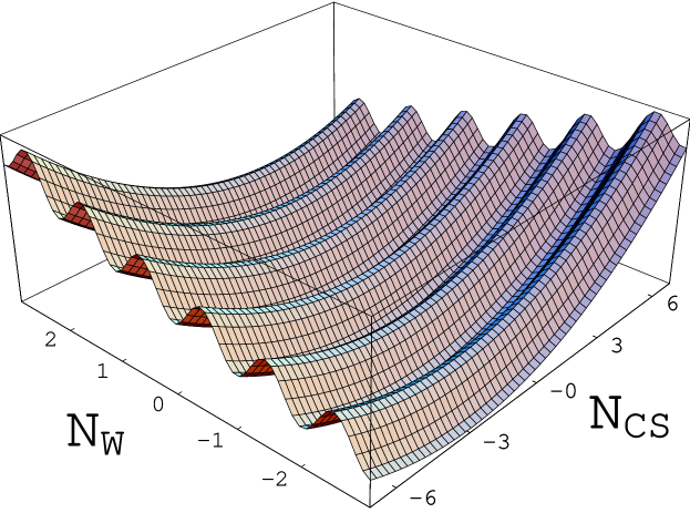
Figure 5: The static system energy $E$ as a function of the Chern-Simons number $N_{{}_{\rm CS}}$ and the winding number $N_{\rm wind}$. Note that $E(N_{{}_{\rm CS}},\;N_{\rm wind})$ is minimal along the vacuum line $N_{{}_{\rm CS}}=N_{\rm wind}$ and increases with $|N_{{}_{\rm CS}}-N_{\rm wind}|$.

Figure 6: Possible paths of topological transitions are shown on the $N_{{}_{\rm CS}}$ – $N_{\rm wind}$ diagram, viewed from above. Path AB represents the simplest non-sphaleronic topological transition in the Higgs sector. See the text for explanation of the notations.

Figure 7: A cross-section of the energy profile at constant $N_{\rm wind}$. The lack of any barriers makes the downward evolution of $N_{{}_{\rm CS}}$ completely unsuppressed. States A and B correspond to the same states in Fig. 6. At non-zero $N_{{}_{\rm CS}}$ the transitions which decrease $|N_{{}_{\rm CS}}-N_{\rm wind}|$ become energetically favorable; a simple case discussed in the text corresponds to the path AB with $N_{{}_{\rm CS}}$ held constant.

Figure 8: Energy profile $E(N_{{}_{\rm CS}},N_{\rm wind})$ along the $N_{\rm wind}$ axis for several values of $N_{{}_{\rm CS}}$. Note that $N_{\rm wind}$ is integer for $any$ field configuration; the curve profile at non-integer $N_{\rm wind}$ reflects the presence of sphaleron-like energy barriers separating the states with $\Delta N_{\rm wind}=\pm 1$. These barriers disappear at sufficiently high $|N_{{}_{\rm CS}}-N_{\rm wind}|$.

As mentioned before, there is no energy barrier for movement along the $N_{{}_{\rm CS}}$ axis, so this movement is completely unsuppressed and controlled by the dynamics of the gauge field condensate $\phi$ according to equation (51). This lack of suppression means that any (potentially large) number of baryons produced by variations in $N_{{}_{\rm CS}}$ would instantly disappear immediately after $N_{{}_{\rm CS}}$ returned to the energetically favorable value $N_{{}_{\rm CS}}=N_{\rm wind}$, provided there were no transitions in Higgs sector ($N_{\rm wind}$ remained unchanged). In other words, even though the fermions are coupled through the anomaly to Chern-Simons number, long-living fermionic states appear only due to transitions in Higgs sector which modify the energy profile along $N_{{}_{\rm CS}}$ axis by moving the center (minimal energy) value of $N_{{}_{\rm CS}}$ around which it oscillates.

As opposed to the absence of barriers for variations in $N_{{}_{\rm CS}}$ only, transitions along the $N_{\rm wind}$ axis require passing over sphaleron-like barriers (for simplicity, the barriers are shown at half-integer values in Fig. 5). Precisely how high this barrier is depends on several circumstances, to be discussed below, notably the Higgs VEV and the spatial scales of the gauge and Higgs fields. In 3+1 dimensions spatially-homogeneous fields have a high barrier (provided the Higgs VEV is not zero), by an argument similar to that given earlier: it would be energetically favorable to separate regions with nontrivial gauge and Higgs fields in sphaleron configuration). In other words, the sphaleron, of size $\sim m^{-1}$, corresponds to the $minimum$ barrier height and the barrier height is greater for all other spatial scales. However, in the 1+1 Abelian Higgs model the barrier at any $N_{{}_{\rm CS}},\;N_{\rm wind}$ is the same as the sphaleron barrier, as can be shown by making a large gauge transformation that eliminates the background gauge field and taking into account that the gauge field component of the 1+1-dimensional sphaleron [23] is inversely proportional to the spatial volume. So the contribution of the gauge field to the (static) energy vanishes at infinite volume, while the Higgs field contribution is identical to that of the sphaleron. The 3+1 dimensional case will be discussed below.

In the homogeneous case discussed in previous sections, when the dimensionless gauge potential $\phi$ is of order one there is both a large Chern-Simons number and a large energy, but zero Higgs winding number $N_{\rm wind}$. It is possible that the energy in a volume containing one unit of Chern-Simons number can exceed the usual sphaleron energy, and (as we show in the next section) this does mean that transitions which change the Higgs winding number become unsuppressed. Note also that literal sphaleron transitions, which change $N_{{}_{\rm CS}}$ and $N_{\rm wind}$ equally, on average do not change the Higgs winding number, which is what is required to produce baryons. These do not change $E(N_{{}_{\rm CS}}-N_{\rm wind})$ and so their rate is not affected by the presence of a nonzero $N_{{}_{\rm CS}}$ density. At any $N_{{}_{\rm CS}}$, the rates of transitions with $\Delta N_{{}_{\rm CS}}=+1$ and $\Delta N_{{}_{\rm CS}}=-1$ equal each other and the contribution of normal topological transitions to total baryoproduction is zero.

7.2 Effective-temperature estimates of transition rates

Here we give some simple estimates of transition rates based on a commonly-used approximation, in which the net rate of baryon production is evaluated from a first-order expansion of the rate in powers of an energy difference, leading to a form in which the rate is evaluated as a zeroth-order sphaleron-like part times a certain energy difference. In order that this be useful, one requires explicit knowledge of this energy dependence. A further simplification, used here, is to assume a Boltzmann dependence with an effective temperature. In Section 7.5 we give an approximate study of the sphaleron-like part of the rate, looking for conditions under which the tunneling barrier to baryoproduction can vanish.

To evaluate the transition rate in the Higgs sector, assume that the transition from zero winding to $N_{\rm wind}=1$ proceeds along $N_{\rm wind}$ axis on the path $AB$ (see Fig. 6). Then the barrier height $E_{+}$ along this path can be estimated as

$$E_{+}=E_{\rm sph}-\left(E(N_{{}_{\rm CS}})-E(N_{{}_{\rm CS}}-1/2)\right)$$ (52)

Similarly, the height of the barrier in the opposite direction is $E_{-}=E_{\rm sph}+(E(N_{{}_{\rm CS}}-1/2)-E(N_{{}_{\rm CS}}-1))$. If one could further assume a Boltzmann distribution with an effective temperature $T_{\rm eff}$, one would obtain different rates $\Gamma_{\pm}$ for transitions in the two directions, with a net rate:

$$\dot{B}/V=\dot{N}_{\rm wind}/V=\Gamma_{+}-\Gamma_{-}\simeq{\Gamma_{\rm sph}\over{2}}{{1}\over{T_{\rm eff}}}\,{{\partial E}\over{\partial N_{{}_{\rm CS}}}}$$ (53)

where $\Gamma_{\rm sph}$ is the sphaleron rate at zero energy change. Then with the help of equations (50,51), the winding number rate of change in 1+1 dimensions is:

$$\dot{N}_{\rm wind}/L=3\pi^{2}\Gamma_{\rm sph}{E_{\rm sph}\over T_{\rm eff}}{n_{{}_{\rm CS}}\over{M_{H}}}$$ (54)

and in (3+1) dimensions:

$$\dot{N}_{\rm wind}/V={\Gamma_{\rm sph}\over T_{\rm eff}}{n_{{}_{\rm CS}}\over{|n_{{}_{\rm CS}}|}}{{2\pi}\over{3\alpha_{W}}}\left(2(8\pi^{2}n_{{}_{\rm CS}})^{1/3}+M_{W}^{2}(8\pi^{2}n_{{}_{\rm CS}})^{-1/3}\right)$$ (55)

(here we assume the barrier height at $N_{\rm wind}=0$ equals $E_{\rm sph}$, and note that the total rate is $\Gamma_{\rm sph}=\Gamma_{+}+\Gamma_{-}$).

It is worth noting that the expression (55) becomes infinitely large at small $n_{{}_{\rm CS}}$. This divergence appears because in 3+1 dimensions the homogeneous $ansatz$ (20)–(23) used throughout the present paper is inadequate for field configurations with small topological charge densities, simply because gauge field configurations with unit Chern-Simons number are localized in space (this is not the case in 1+1 dimensions).

Strictly speaking, it is unclear whether the topological transitions in Higgs sector proceed along the $N_{\rm wind}$ axis or along the maximal gradient direction orthogonal to the $N_{\rm wind}=N_{{}_{\rm CS}}$ line. However, the energy gains $E_{\pm}-E_{\rm sph}$ in the latter case are larger only by factor of 2, which makes no qualitative difference in our analysis.

With the increase in $N_{{}_{\rm CS}}-N_{\rm wind}$ the energy gain obtained by transitions with $N_{\rm wind}=\pm 1$ also increases, so at very large values of $N_{{}_{\rm CS}}-N_{\rm wind}$ transitions along the $N_{\rm wind}$ axis also become unsuppressed because the energy gain (52) becomes equal to or greater than the barrier height, i.e., the energy of a sphaleron-like Higgs configuration. The critical values can be estimated by putting $E_{-}=0$ in (52) and using equations (50,51):

$$n_{{}_{\rm CS}}^{crit}\sim{2\over{3\pi^{2}}}M_{H}={2\over{3\pi^{2}}}{L_{\rm sph}}^{-1}$$ (56)

In proper dimensionless units [22] equation (56) becomes $n_{{}_{\rm CS}}^{crit}\sim 1/10$ or $A_{1}\sim 1/2$) in 1+1 dimensions and

$$n_{{}_{\rm CS}}^{crit}\sim{1\over{2\pi^{2}}}m^{3}$$ (57)

in 3+1 dimensions, which is about $1/(2\pi^{2})$ per sphaleron volume. Equation (57) is equivalent to $\phi\raisebox{-3.44444pt}{\mbox{$\stackrel{{\scriptstyle\textstyle>}}{{\sim}}$}}1$, comparable to the maximum amplitudes of $\phi$ seen in the numerical simulations.

7.3 Baryoproduction

Let us give some simple estimates of baryon production in the 1+1 Abelian Higgs model. Taking into account that the number of long-living fermionic states is equal to the net shift of Higgs winding number, and using equation (54), one obtains

$$\dot{B}=3\pi^{2}{E_{\rm sph}\over{M_{H}}}{\Gamma_{\rm sph}\over T_{\rm eff}}n_{{}_{\rm CS}}L$$ (58)

and

$$\Delta B=3\pi^{2}{E_{\rm sph}\over{M_{H}}}\int dt\,{\Gamma_{\rm sph}\over T_{\rm eff}}n_{{}_{\rm CS}}L$$ (59)

where $\Delta B$ is the total number of generated baryons.

Although the detailed discussion of $\Gamma_{\rm sph}$ and $T_{\rm eff}$ time dependence goes beyond the scope of this paper, there are no reasons to expect any qualitative difference from previous studies [3, 4, 11]. There it was argued that $\Gamma_{\rm sph}/T_{\rm eff}$ is a smooth function of time with a sharp increase at the beginning of preheating and a slow decrease in the course of thermalization to the final reheating temperature. The exact timing depends on initial conditions. However, equation (59) provides a simple way to check how efficient the baryoproduction is for any reasonable time evolution of $\Gamma_{\rm sph}$ and $T_{\rm eff}$. As long as the frequency of $N_{{}_{\rm CS}}$ oscillations is much larger the inverse thermalization time, we may substitute $\Gamma_{\rm sph}/T_{\rm eff}$ by 1 in the right-hand side of equation (59) which turns into the integrated average of Chern-Simons number density

$$\langle n_{{}_{\rm CS}}(t)\rangle=\int_{0}^{t}dt\,n_{{}_{\rm CS}}(t)$$ (60)

Time intervals when $\langle n_{{}_{\rm CS}}(t)\rangle$ remains constant give zero baryoproduction; an increase or decrease in $\langle n_{{}_{\rm CS}}(t)\rangle$ corresponds to a nonzero secular average of $N_{{}_{\rm CS}}$ and thus to positive or negative baryoproduction (provided the transition rate $\Gamma_{\rm sph}(t)$ is nonzero). The simplest way to get a nonzero $N_{{}_{\rm CS}}$ secular average is to introduce a bias or tilt in $E(N_{{}_{\rm CS}})$ through CP-violating terms either directly coupled to $N_{{}_{\rm CS}}$ in the bosonic Lagrangian, as in equation (10), or coupled to the fermion density operator of equation (8) which modifies $E(N_{{}_{\rm CS}})$ through the anomaly. It is also possible to shift the time average of $N_{{}_{\rm CS}}$ in other ways through dynamical effects already described in section 5.

7.4 Washout from fermion backreaction

Washout is one of the most prominent forms of fermionic backreaction. As long as the topological transitions keep going, newly-created baryons tend to disappear through the same anomaly mechanism that created them, to the extent that the decrease of fermionic density reduces the system energy. Washout (in 1+1 dimensions) can be accounted for by adding a dissipative term to equation (58):

$$\dot{B}=3\pi^{2}{E_{\rm sph}\over{M_{H}}}{\Gamma_{\rm sph}\over T_{\rm eff}}n_{{}_{\rm CS}}L-\Gamma_{B}B$$ (61)

where the dissipation rate $\Gamma_{B}$ is generally proportional to the sphaleron rate $\Gamma_{\rm sph}$. In 3+1 dimensions [3],

$$\Gamma_{B}={39\over 2}{\Gamma_{\rm sph}\over{T_{\rm eff}^{3}}}$$ (62)

The solution of equation (61) can be found in the form (compare to equation (59)):

$$\Delta B=3\pi^{2}{E_{\rm sph}\over{M_{H}}}e^{-\gamma(t)}\int_{0}^{t}d\tau\,e^{\gamma(\tau)}{{\Gamma_{\rm sph}(\tau)}\over T_{\rm eff}(\tau)}n_{{}_{\rm CS}}(\tau)L$$ (63)

(here $\gamma(t)=\int_{0}^{t}d\tau\,\Gamma_{B}(\tau)$). Direct use of equations (61,63) appears to be problematic in our simulations for two reasons. First, explicit time dependences of the rate $\Gamma_{\rm sph}$ and the effective temperature $T_{\rm eff}$ are controlled by dynamics in the inflaton and Higgs sector which are beyond the scope of the present paper. Second, equation (61) assumes the fermions to be thermalized, which obviously is not the case if Chern-Simons number oscillates with frequency of order of $m$.

However, it is easy to see that solution (63) decays exponentially with time if $n_{{}_{\rm CS}}=0$ and $\Gamma_{B}\neq 0$. Therefore, it is desirable to keep baryoproduction going until the topological transitions end (e.g. because of freeze-out during thermalization to a low reheating temperature). Otherwise, if baryoproduction ends before the sphaleron transition rate approaches zero, wash-out could crucially affect the final density of baryons.

Again, the time dependence of the $n_{{}_{\rm CS}}$ running average (60) provides important information about the baryoproduction period and allows one to estimate acceptable thermalization times. For example, short-term baryoproduction followed by stabilization of $\langle n_{{}_{\rm CS}}(t)\rangle$ at a certain value (see Fig. 2) would seldom survive the wash-out, while steady baryoproduction (such as is shown in Fig. 3) leaves ample time for the sphaleron transitions to freeze.

7.5 Dependence of tunneling barriers on $\phi$ and scale sizes

Our purpose here is to find approximately the conditions under which the tunneling barrier in the sphaleron rate $\Gamma_{\rm sph}=\Gamma_{+}+\Gamma_{-}$ (see equation (53)) can vanish. It will not be necessary to use an effective-temperature approximation. The techniques used here, based on work of a decade or more ago [25, 26, 27, 12] on topological charge-changing transitions, are qualitative but useful. They go beyond ’t Hooft’s original work, whose famous tunneling factor of $\exp[-8\pi^{2}/g^{2}]$ holds only at zero energy and, at that energy, is (classically) independent of scale size. We give an approximate barrier-factor formula with explicit dependences on energy, scale size, and Higgs VEV, and outline the regions of this parameter space where the tunneling exponent can vanish. We do not discuss the origin or distribution of spatial scales, but simply assumes that these arise through some mechanism such as the unstable growth of spatial ripples [8].

There are other interesting approaches to this kind of problem, which we intend to investigate in the future. These include studies of non-Abelian gauge dynamics in the presence of a non-vanishing topological charge density [28] or in the presence of a time-varying electric background potential [29], and a study of the conversion of a time-varying background topological charge to fermions through the anomaly [30]. These works use various specialized backgrounds not exactly comparable to the Chern-Simons condensate used in the present paper, but they should still have qualitative applicability.

There are at least two mechanisms which can remove tunneling barriers, and these may operate at the same time. The first mechanism is generally important for large scale sizes (large means compared to the vacuum W-boson mass); it involves swinging of the Higgs VEV through zero. The second mechanism involves selection of a spatial scale such that the original Chern-Simons condensate is well-matched to baryon production through the anomaly. As one might expect, the best overlap occurs when the size scale is about $m^{-1}$, and the corresponding configurations are somewhat like sphalerons in size, but it is apparently possible for tunneling barriers to be overcome at considerably larger spatial scales. However, baryon production is inefficient at these large scales.

First we discuss the conditions for no tunneling barriers with a fixed and finite W-boson mass $m$, and then remark briefly on what happens when there is no mass because the Higgs VEV vanishes.

7.5.1 The no-barrier condition for finite W-boson mass

There must be a transformation of Chern-Simons number from the spatially-homogeneous condensate to one characterized by spatial inhomogeneities such as sphalerons. That is, in the expression for $N_{{}_{\rm CS}}$

$$N_{{}_{\rm CS}}=\frac{-1}{8\pi^{2}}\int d^{3}x\epsilon_{ijk}{\rm\,Tr\,}[A_{i}\partial_{j}A_{k}+\frac{2}{3}A_{i}A_{j}A_{k}]$$ (64)

the relevant sphaleron-like configurations of the $A_{i}$ are typified by gauge potentials which approach at infinity pure-gauge terms carrying winding number; the Higgs field carries the same winding number for a minimum-energy configuration. The gauge in question was termed $U$ in equations (48, 49).

A typical form for a gauge matrix $U$ carrying unit winding number is [25, 26]:

$$U=\exp\left[\frac{i}{2}\vec{\tau}\cdot\hat{r}\beta(r,t)];\;\;\beta(r,t)=2\arctan[r/\lambda(t)\right]$$ (65)

where $\lambda(t)$ is a monotonic function of $t$ going to $-\infty$ at $t=-\infty$ and to $\infty$ at $t=\infty$. A gauge matrix for Chern-Simons number $N_{{}_{\rm CS}}$ is simply a product of $N_{{}_{\rm CS}}$ terms of the form (65) translated to various spatial and temporal centers. We will refer to the spatially-homogeneous gauge potentials dealt with in earlier sections as $\phi$ form potentials, and the spatially-dependent sphaleron-like configurations as $U$ form potentials. Of course, either form is at best an approximation; the $\phi$ form potentials will develop spatial gradients by several mechanisms, and the $U$ form potentials will not literally be of the approximate form we use below.

Long ago, Bitar and Chang [25] constructed Minkowski-space gauge potentials of unbroken $SU(2)$ gauge theory whose asymptotic behavior was precisely that of equation (65). They chose the single dynamical degree of freedom to be the function $\lambda(t)$ of this equation; the non-asymptotic gauge potential is further parameterized by a non-dynamical scale coordinate and translation coordinates. The parameterization is conveniently written as:

$$A_{\mu}=\left(\frac{r^{2}+\lambda^{2}}{r^{2}+\lambda^{2}+\rho^{2}}\right)U\partial_{\mu}U^{-1}$$ (66)

where $\rho$ is the scale coordinate (we will not need to display the translation coordinates, which we set to zero). Bitar and Chang [25] show that the topological charge of this potential is unity for any scale coordinate value. They also show that the dynamical degree of freedom $\lambda$ has a Hamiltonian which is quadratic in $\dot{\lambda}$ but a complicated function of $\lambda$, and computed the barrier exponent $\int pdq$ at zero energy from this Hamiltonian, recovering the ’t Hooft result. Later this work was extended [26] to EW theory with a Higgs field (as well as a chemical potential for Chern-Simons number); this work then formed the basis [13] for an investigation of scattering processes involving topological charge change at very high energies. In this paper, we extend these earlier works to cover the entire range of scale coordinates (Ref. [13] only covered the regime of small scale coordinates).

We wish to find the conditions under which the corrugations or barrier factors described in connection with Fig. 5 vanish, within a framework general enough to go beyond thermal quasi-equilibrium. Begin with a general formula of Cline and Raby [27] for the diffusive rate. Originally the Cline-Raby formula was given for thermal equilibrium conditions, but it is easily modified for non-equilibrium conditions. The derivation is slightly different from Cline and Raby’s because of the non-equilibrium nature of the process. Consider diffusive dynamics of the Chern-Simons number $N_{{}_{\rm CS}}(t)$ in which the diffusion constant $\Gamma$ can be written in the usual form:

$$\frac{\Gamma}{V}=\frac{1}{2V}\int^{\infty}_{-\infty}\langle\dot{N}_{{}_{\rm CS}}(t)\dot{N}_{{}_{\rm CS}}(0)\rangle=\frac{\pi}{V}\sum_{if}\rho(i)\delta(E_{f}-E_{i})|\langle i,E_{i}|\dot{N}_{{}_{\rm CS}}(0)|f,E_{f}\rangle|^{2}$$ (67)

where $V$ is the volume of space and the brackets refer to a trace over the density matrix; this density matrix is, for the present purposes, taken to be diagonal in the energies $E_{i},E_{f}$ of the states summed over, with entries $\rho(i)$. In fact, the density matrix is changing in time and so does not commute with the Hamiltonian, but at the present level of (in)accuracy this is an inessential complication. Cline and Raby take the $i$ states to be in states at $t=-\infty$ and the $f$ states to be out states at $t=+\infty$, and then use the formula:

$$\int^{\infty}_{-\infty}dt\langle i,E_{i}|\dot{N}_{{}_{\rm CS}}(t)|f,E_{f}\rangle=2\pi\delta(E_{i}-E_{f})\langle i,E_{i}|\dot{N}_{{}_{\rm CS}}(0)|f,E_{f}\rangle$$ (68)

$$=\langle i,E_{i}|N_{{}_{\rm CS}}(\infty)-N_{{}_{\rm CS}}(-\infty)|f,E_{f}\rangle=i\Delta N_{fi}(2\pi)^{4}\delta_{4}(p_{f}-p_{i})T_{fi}$$

where $T_{fi}$ is the zero-temperature S-matrix element from the initial to the final state, and $\Delta N_{fi}$ is the change in Chern-Simons number (or topological charge) from the initial to the final state. Substitution in (68) yields:

$$\frac{\Gamma}{V}=\frac{1}{2}\sum_{if}\rho(i)(2\pi)^{4}\delta_{4}(p_{f}-p_{i})(\Delta N_{fi})^{2}|T_{if}|^{2}.$$ (69)

Further progress depends on analysis of B+L-violating S-matrix elements at zero temperature, a subject of some considerable interest a decade ago (see, e.g., [12]). Ref. [13] gives the following very crude approximation to the $|\Delta N_{fi}|=1$ S-matrix elements at fixed energy $E$:

$$T_{if}\sim(\frac{4\pi^{2}}{g})^{N}\int_{0}^{\infty}d\rho\rho^{N-5}\prod_{j}e^{-\rho k_{j}}e^{-Q(\rho,E)}$$ (70)

where $Q$ is a barrier exponent, $N$ is the total number of particles involved in the scattering process, $\rho$ is a scale collective coordinate, and $k_{j}$ is the magnitude of the three-momentum of particle $j$. This formula is based on a transcription of familiar Euclidean formulas for scattering in the presence of instantons to Minkowski space. Unlike naive instanton-based amplitudes, the above amplitudes $T_{if}$ behave properly at high energy (where one expects $\rho\simeq N/E$) but are not correctly unitarized; this will not be an important issue here.

The barrier exponent $Q$ was originally [13] given for small $\rho$. The appropriate expression for all $\rho$ can straightforwardly found using the techniques of [25, 26]:

$$Q(\rho,E)=\frac{6\pi^{2}}{g^{2}}\int_{-\infty}^{\infty}d\xi F(\xi)^{1/2}\Theta[F(\xi)],$$ (71)

where the function $F$ is:

$$F(\xi)=(\xi^{2}+1)^{-5/2}[(\xi^{2}+1)^{-5/2}+m(t)^{2}\rho^{2}f(\xi)-\frac{1}{3\pi^{2}}E\rho g^{2}].$$ (72)

Here we make it explicit that the W-boson mass $m(t)$ depends on time, because the Higgs field depends on time. The function $f(\xi)$ is not expressible analytically, but one can show that $f$ is positive and obeys $f(\xi)\leq f(0)=4/3$.

The barrier factor $Q$ vanishes if the function $F$ is always negative, which happens for certain regimes of energy $E$, mass $m(t)$, and scale coordinate $\rho$. Clearly, there is always a finite barrier at $\rho=0$ (just the ’t Hooft barrier if $m$=0). For non-zero $\rho$ it is generally true that if $F(\xi=0;\rho,m,E)$ vanishes then $F\leq 0$ for all $\xi$. The no-barrier condition then is:

$$1+\frac{4m^{2}\rho^{2}}{3}-\frac{E\rho g^{2}}{3\pi^{2}}\leq 0.$$ (73)

Consider first the usual case where $m$ is the standard W mass. The minimum energy $E$ yielding equality in equation (73) occurs at $\rho=\sqrt{3}/2m,\;E_{min}=4\pi^{2}\sqrt{3}m/g^{2}$. This minimum should be the sphaleron energy, and it is indeed a very good numerical approximation [26] in the limit of large Higgs mass.

Next we take up the case where the W mass, or Higgs VEV, is near zero.

7.5.2 Higgs VEV near zero

It appears that large scales $\rho$, which would be expected in the first stages of transition of Chern-Simons number from $\phi$ form to $U$ form, will have a disastrously large barrier factor going like $\exp(-{\rm const}\;m\rho/g^{2})$, if the mass $m$ is anywhere near its standard value. However, if—as discussed in Sec. 5A—the Higgs field $v$ oscillates through zero because of gauge back reaction, the gauge mass $m=gv/2$ vanishes and the barrier $Q$ will vanish periodically (see (72) at energies $E\sim 1/(\rho g^{2})$; that is, more easily at large scales than at small. So Higgs oscillations are one potentially-vital means of generating baryons from Chern-Simons number. It is easy to check that if the barrier factor is unity for a time $\tau$ during a Higgs oscillation period $\tau_{\rm Higgs}$, the averaged barrier factor over a Higgs period is not exponentially small, but is of order $\tau/\tau_{\rm Higgs}$.

Unfortunately, this is not the end of the story, since there are other possible suppression effects to deal with; a poor overlap of anomaly-produced baryons with the Chern-Simons condensate can be disastrous.

7.6 Good overlap condition

Here we explore how the conditions of both no barrier as well as a good overlap between a $U$ form potential and baryons produced through the anomaly can be satisfied.

Even if $v$ does not vanish during preheating it is possible in principle to have a zero barrier factor, depending on what values of the dimensionless gauge potential $\phi$ are reached. Values of $|\phi|$ near or slightly greater than one are fairly readily gotten, as is evident from the structure of the equations of motion and from the numerical studies reported above, and for such values of $\phi$ there need be no barrier. However, it is possible for $|\phi|$ to be small compared to unity; we explore that possibility here. As one might expect, for values of $\phi$ rather less than one, it requires a rather large region to gather together enough energy to overcome the barrier. It will turn out that spatial scales much larger than the inverse of the vacuum W-boson mass are self-consistent only if the Higgs VEV does go near zero.

Consider a region of space of size $\rho$ as defined by gradients appearing during preheating and further unstable amplification. In this region the total energy and Chern-Simons number are approximately:

$$E(\rho)\simeq\frac{4\pi m}{g^{2}}(m\rho)^{3}(\phi^{2}+\phi^{4});\;\;N_{tot}(\rho)\simeq\frac{(m\rho\phi)^{3}}{6\pi}.$$ (74)

Inserting these estimates in the no-barrier condition (73) yields:

$$(m\rho)^{2}=\frac{\pi}{2(\phi^{2}+\phi^{4})}\left\{1+[1+\frac{3}{\pi}(\phi^{2}+\phi^{4})]^{1/2}\right\}\simeq\frac{\pi}{\phi^{2}},$$ (75)

with the last form holding for small $|\phi|$. In this case the total energy and Chern-Simons number in terms of $\phi$ are:

$$E=\frac{4\pi^{5/2}m}{g^{2}|\phi|};\;N_{tot}=\frac{\pi^{1/2}}{6}=O(1).$$ (76)

The appearance of inverse powers of $\phi$ suggests the inefficiencies of avoiding a barrier when parametric resonance amplification of the EW gauge potential is small: The energy is large compared to the sphaleron mass, but the change in B+L is only of order one (per unit flavor). Still, these inefficiencies could be tolerable in view of the exponentially-small efficiency of actual barrier penetration. When amplification leads to $|\phi|\sim 1$, avoiding a barrier is rather like having energy at or above the sphaleron mass.

Next turn to the conditions specifying a good overlap between the $\phi$ condensate and baryogenesis. We will find that a good overlap means $|\phi|$ cannot be too far below unity, but we cannot quantify this statement with the present crude approximations. The point of a good overlap is that having an energy larger than the barrier energy is by no means sufficient in many cases to lead to unsuppressed B+L violation, as many authors have discussed [12, 13]. For example, in the formula (70) for S-matrix elements, the other factors integrated over $\rho$ in that equation can lead to suppression of the S-matrix element by a factor of order $\exp[-\zeta 8\pi^{2}/g^{2}]$ with $\zeta\sim 1/2$ or so [13]. This sort of suppression even in the absence of a tunneling barrier comes about because of a very poor overlap between multi-particle initial and final states when these have very different numbers of particles and at least one particle number is very large. When the states are sufficiently similar there is no such extra suppression, which is what happens in thermal equilibrium at large enough temperature. In the present case something similar happens. The initial state in the Cline-Raby formula (68,69) is not a conventional particle state; it is a coherent state somewhat similar to the $\phi$ form potential, but with a spatial size $\rho$ coming from various effects, such as growth of unstable momentum modes [8]. If this state has a large overlap with the $U$ form potentials such as in (66), and if there is no barrier for tunneling, then the amplitude for baryon creation will be unsuppressed. One can say that the exponentially-small rate of B+L violation in $2\rightarrow N$ collisions stems from the Drukier-Nussinov effect [14] that it is extremely unlikely for a two-particle collision state to couple well to a soliton like the sphaleron, but in our case the Chern-Simons condensate may, for certain values of $\phi$ and $\rho$,look enough like a “soliton” for there to be good overlap.

We seek this substantial overlap between a generic $\phi$ form potential, somehow modified to have an overall spatial scale $\rho$, and a $U$ form (Bitar-Chang) potential, when $\rho$ is a large scale compared to other spatial scales. At large $\rho$ the Bitar-Chang fields scale as:

$$gE\sim\frac{\dot{\lambda}}{\rho^{2}};\;gB\sim\frac{1}{\rho^{2}}.$$ (77)

By comparisonto the $\phi$ form potentials of equation (22) one sees from the B field consistency with the relation $m\rho\sim 1/|\phi|$, and that consistency with the E field can be achieved if $\lambda\sim\ln\phi$.

Now return to the approximate form of the S-matrix elements (70). The process to be described is the transformation of a $\phi$ form field with certain spatial scales to a final state of $N$ particles, including a set of particles which violates B+L. The process is only interesting if there is no tunneling barrier, so we assume the validity of equation (73). The next question to ask is whether one can, consistent with (73), argue for a non-suppressed overlap between the modified $\phi$ form and the final state. In the crude approximation of equation (70) this simply amounts to asking whether the constraint on scale coming from the final-state wave function is consistent with other information on that scale, such as the condition (73) for no barrier. In (70) there occurs a product of exponentials of the type $\exp(-k_{i}\rho)$ where $k_{i}$ is the spatial momentum of the $i^{th}$ particle. It is reasonable to assume that all the particles are effectively massless, and then the product of wave functions reduces to $\exp(-E\rho)$. One easily sees that, if the barrier exponential factor $\exp-Q$ is unity, the $\rho$ integrand maximizes at $\rho=N/E$, just as estimated [13] for more conventional S-matrix elements. So a good overlap simply means that the number of produced particles is (more or less) determined. This turns out, taking into consideration the no-barrier condition (76), to yield $N\sim 1/g^{2}\phi^{2}$. (One might argue that in fact particles do have mass, and so one should have $N\leq E/M\sim 1/g^{2}|\phi|$ which would require $|\phi|$ at least of order unity. However, $m$ is the W-boson mass, and all baryons and leptons except for baryons with top quarks are not nearly that heavy.)

As in [13] we can form a rate from the Cline-Raby formula 69 by multiplying the squared S-matrix elements from (70) by massless $N$-particle phase space [13]. Nothing quantitative should be trusted about the resulting equation (78) below, except for its dependence on $\phi$:

$$\frac{\Gamma}{V}\sim\frac{E^{4}}{N!g^{2N}}\sim(\frac{m}{g^{2}\phi})^{4}(\frac{\phi^{2}}{\phi_{c}^{2}})^{N}.$$ (78)

Here $\phi_{c}$ is a critical value of $\phi$ separating small from large rates (in the present highly inaccurate approximation, $\phi_{c}^{2}=e^{-1}$). Whatever $\phi_{c}$ is, and it is evidently of order unity, it is clear that for $N\geq 2$ and for $\phi^{2}\geq\phi_{c}^{2}$ the B+L process is unsuppressed, while in the opposite limit it is strongly suppressed. Note that if the dimensionless potential $\phi$ is of order unity the energy scale is the sphaleron mass and the spatial scale is $m^{-1}$. So we conclude, not unexpectedly, that if the Higgs VEV is not oscillating near zero spatial scales near the sphaleron mass must be formed; if the Higgs field is oscillating near zero, much larger spatial scales will serve for unsuppressed B+L production.

8 Conclusions

In this work we studied a scenario of baryogenesis in the Standard Model, based on inflation on EW scales with the Higgs coupled to the oscillating inflaton in a preheating phase. If baryons could be generated, they could be saved from washout at reheating because the reheat temperature is less than the EW cross-over temperature where sphaleron washout can be large, so the topological transitions can completely freeze out before the preheating ends. However, the dynamics of conversion of Chern-Simons condensate to B+L and the dynamics of washout of this B+L are very complex and not yet well-understood.

Although we have no rigorous proof that B+L production involving only standard-model fields (coupled to the inflaton) is truly viable, we can at least say that so far that we have not identified any mechanisms which rule out a pure EW/inflaton scenario.

Extending the earlier work of Ref. [8], we added explicit CP violation to the spatially-homogeneous classical gauge equations of motion, rather than (as in [8]) depending only on initial value of the functions $\phi,\dot{\phi}$ for CP violation. The effects of explicit CP-violating terms was studied analytically in some simple models, as well as numerically. We studied numerically the classical dynamics of the Higgs field, including classical back reaction of the gauge field on the Higgs field.

The gauge reaction on the Higgs equation of motion is important in two respects: It can broaden parametric resonances by getting away from pure sinusoidal variation of the Higgs field, which was the only case considered in [8]. And it can, as discussed above, lead to conversion of Chern-Simons number to baryons which for some fraction of the time is unsuppressed by tunneling barriers, since gauge backreaction often modifies the Higgs potential and causes the Higgs field to oscillate through zero, rather than staying at the bottom of the potential well.

There are various forms of CP violation which could be added to the equations of motion; we explored three in the gauge equations and one in the Higgs equation. In the gauge sector one came from strong out-of-equilibrium CP violation; another came from a multi-Higgs sector with spontaneous CP violation; and the third was a higher-derivative CP-violating term, which could be associated with other lower-dimension operators. In the Higgs sector we explored spontaneous baryogenesis in a multi-Higgs model, leading to an effective chemical potential for baryons. Generally speaking, the resultant secular average of the Chern-Simons number is a few orders of magnitude less than the dimensionless coefficient multiplying the CP-violating term in the gauge equations of motion.

Formation of a spatially-homogeneous Chern-Simons condensate is only the beginning of the story; it is necessary to convert this condensate into something resembling a condensate of sphalerons of the same Chern-Simons number, in order to generate the Higgs winding number which is converted to baryons. The usual approach of invoking a thermal (or effectively thermal) regime immediately following the parametric resonance regime is not likely to be applicable. A quantitatively-adequate study of these non-thermal non-equilibrium processes remains to be done, but we have given useful criteria for evading the two possible process which lead to exponential suppression of baryogenesis. The first, of course, is the topological-charge tunneling barrier. The second is a poor overlap between initial and final states in a process even with no barrier. Based on earlier work which studied the (im)possibility of baryon production in accelerator collisions, we gave crude estimates of the parameter ranges which avoid both barriers and bad overlap, and pointed out the influence of the Higgs VEV passing near zero for these parameter ranges. The conclusion is that if the Higgs VEV stays near its vacuum value, spatial scales near the vacuum inverse W-boson mass and energies near the vacuum sphaleron mass can avoid both forms of suppression, quite unlike the $2\rightarrow N$ collision case where poor overlap cannot be avoided. If this VEV goes near zero, the spatial scales can be larger and the energy scales smaller.

If this view proves to be correct, the rate-limiting step in baryogenesis will be the conversion of $\phi$ form EW fields to $U$ form fields, by growth of perturbations at various spatial scales.

The scenario of regions of almost spatially-homogeneous Chern-Simons condensate of order of the EW Hubble size, may have consequences beyond B+L generation. It has been proposed [33] that any mechanism of B+L generation involving the EW anomaly will leave its trace on the early universe through large-scale helicity of the Maxwell magnetic fields which descend from EW gauge fields as the universe cools. As is well-known, if these magnetic fields have typical EW scales of $10^{-16}$ cm, the present-day magnetic-field scale will be far too small even taking expansion of the universe into account. Following earlier studies in magnetohydrodynamics, Ref. [33] proposed that the helicity would drive an inverse cascade to longer scales. This idea was further pursued by Son and by Field and Carroll [34]. If the EW fields which lead to Maxwell magnetic fields are generated on the EW Hubble size scale, one gains many orders of magnitude toward seeding present-day intergalactic magnetic fields by EW processes. Moreover, there might be much more Maxwell helicity than the minimum required to produce the present-day abundance of baryons, since only a fraction of the $\phi$ form Chern-Simons condensate will be turned into baryons. The Maxwell helicity produced during preheating amplification of CP violation can be very much greater than the number of baryons. Work is underway to investigate these points.

Acknowledgments

This work was supported in part by the US Department of Energy, grant DE-FG03-91ER40662, Task C, and by the NATO Collaborative Linkage Grant PST.CLG.976397. D. G. thanks the Elementary Particle Theory group of UCLA, where this work was performed, for their kind hospitality during his visit; his work is supported in part by CRDF grant RP1-2103. D. G. is indebted to N. Manton, S. Nussinov and M. Shaposhnikov for discussions and comments.

References

- [1] L. Kofman, A. Linde, and A. A. Starobinsky, Phys. Rev. Lett. 73, 3195 (1994), ibid. 76, 1011 (1996); Phys. Rev. D 56, 3258 (1997).
- [2] L. M. Krauss and M. Trodden, Phys. Rev. Lett.83, 1502 (1999).
- [3] J. García-Bellido, D. Grigoriev, A. Kusenko, and M. Shaposhnikov, Phys. Rev. D 60, 123504 (1999).
- [4] J.García-Bellido and D.Grigoriev, JHEP0001, 017 (2000).
- [5] G. Germán, G. Ross, and S. Sarkar, hep-ph/0103243.
- [6] V. A. Kuzmin, V. A. Rubakov, and M. Shaposhnikov, Phys. Lett. 155B, 36 (1985).
- [7] A. Cohen, D. Kaplan, and A. Nelson, Ann. Rev. Nucl. Part. Sci. 43, 27 (1993).
- [8] J. M. Cornwall and A. Kusenko, Phys. Rev. D 61, 103510 (2000).
- [9] A. G. Cohen, D. B. Kaplan and A. E. Nelson, Phys. Lett. B 263, 86 (1991).
- [10] T. D. Lee, Phys. Rev. D 8, 1226 (1973); Phys. Reports 9, 143 (1974); S. Weinberg, Phys. Rev. Lett. 37, 657 (1976).
- [11] D. Grigoriev, in Proceedings of the 35th Rencontres de Moriond, hep-ph/0006115.
- [12] Baryon Number Violation at the SSC, Proceedings of the Santa Fe Workshop, ed. M. Mattis and E. Mottola (World Scientific, Singapore, 1990).
- [13] J. M. Cornwall, Phys. Lett. B 243, 271 (1990).
- [14] A. K. Drukier and S. Nussinov, Phys. Rev. Letters 49, 102 (1982).
- [15] P. Hänggi and R. Bartusek, in Lecture Notes in Physics, Vol. 476, ed. J. Parisi, S. C. Müller, and W. Zimmerman (Springer, New York, 1996), p. 294.
- [16] A. Rajantie and E. J. Copeland, Phys. Rev. Letters 85, 916 (2000).
- [17] A. Rajantie, P. M. Saffin, and E. J. Copeland, hep-ph/0012097.
- [18] D.Yu. Grigoriev, M. Shaposhnikov and N. Turok, Phys. Lett. B 275, 395 (1992).
- [19] M. Dine and S. Thomas, Phys. Lett. B 328, 73 (1994) [hep-ph/9401265]; D. Comelli, M. Pietroni and A. Riotto, Phys. Lett. B 354, 91 (1995) [hep-ph/9504265]; Phys. Rev. D 53, 4668 (1996) [hep-ph/9506278]; P. Huet and A. E. Nelson, Phys. Rev. D 53, 4578 (1996) [hep-ph/9506477].
- [20] R. Brustein and D. H. Oaknin, Phys. Rev. Lett. 82, 2628 (1999) [hep-ph/9809365]; Phys. Rev. D 60, 023508 (1999) [hep-ph/9901242]; hep-ph/0003166.
- [21] E. Witten, Nucl. Phys. B156, 269 (1979); G. Veneziano, Nucl. Phys. B159, 213 (1979).
- [22] D. Yu. Grigoriev, V.A. Rubakov and M. E. Shaposhnikov, Phys. Lett. B216, 172 (1989); Nucl. Phys. B326, 737 (1989).
- [23] A. I. Bochkarev and M. E. Shaposhnikov, Mod. Phys. Lett. A 2, 991 (1987) [Erratum-ibid. A 4, 1495 (1987)]; D. Yu. Grigoriev and V. A. Rubakov, Nucl. Phys. B 299, 67 (1988).
- [24] S. Yu. Khlebnikov and M. E. Shaposhnikov, Nucl. Phys. B 308, 885 (1988); V. A. Rubakov and M. E. Shaposhnikov, Usp. Fiz. Nauk 166, 493 (1996) [Phys. Usp. 39, 461 (1996)]; G. D. Moore, Nucl. Phys. B 480, 657 (1996).
- [25] K. M. Bitar and S.-J. Chang, Phys. Rev. D 17, 486 (1978).
- [26] J. M. Cornwall, Phys. Rev. D 40,4130 (1989).
- [27] J. Cline and S. Raby, Phys. Lett. B 246, 163 (1990).
- [28] A. I. Nikishov, hep-th/0104019.
- [29] G. C. Nayak, D. D. Dietrich, and W. Greiner, hep-ph/0104030.
- [30] F. R. Klinkhamer and Y. J. Lee, hep-th/0104096.
- [31] N. Hatzigeorgiou and J. M. Cornwall, Phys. Lett. B 327, 313 (1994).
- [32] S. Khlebnikov, L. Kofman, A. Linde and I. Tkachev, Phys. Rev. Lett. 81, 2012 (1998).
- [33] J. M. Cornwall, Phys. Rev. D 56, 6146 (1997).
- [34] D. T. Son, Phys. Rev. D 59, 063008 (1999); G. B. Field and S. M. Carroll, Phys. Rev. D 62, 103008 (2000).