Q-ball formation: Obstacle to Affleck-Dine baryogenesis
in the gauge-mediated SUSY breaking ?

Abstract

We consider the Affleck-Dine baryogenesis comprehensively in the minimal supersymmetric standard model with gauge-mediated supersymmetry breaking. Considering the high temperature effects, we see that the Affleck-Dine field is naturally deformed into the form of the Q ball. In the natural scenario where the initial amplitude of the field and the A-terms are both determined by the nonrenormalizable superpotential, we obtain only very a narrow allowed region in the parameter space in order to explain the baryon number of the universe for the case that the Q-ball formation occurs just after baryon number production. Moreover, most of the parameter sets suited have already been excluded by current experiments. We also find new situations in which the Q-ball formation takes place rather late compared with baryon number creation. This situation is more preferable, since it allows a wider parameter region for naturally consistent scenarios, although it is still difficult to realize in the actual cosmological scenario.

]

I Introduction

The Affleck-Dine (AD) mechanism [1] is the most promising scenario for explaining the baryon number of the universe. It is based on the dynamics of a (complex) scalar field $\phi$ carrying baryon number, which is called the AD field. During inflation, the expectation value of the AD field develops at a very large value. After inflation the inflaton field oscillates about the minimum of the effective potential, and dominates the energy density of the universe like matter, while the AD field stays at the large field value. It starts the oscillation, or more precisely, rotation in its effective potential when $H\sim m_{\phi,eff}$, where $H$ and $m_{\phi,eff}\equiv|V^{\prime\prime}(\phi)|$ are the Hubble parameter and the curvature of the potential of the AD field. Once it rotates, the baryon number will be created as $n_{B}\sim\omega\phi^{2}$, where $\omega=\dot{\theta}$ is the velocity of the phase of the AD field. When $t\sim\Gamma_{\phi}$, where $\Gamma_{\phi}$ is the decay rate of the AD field, it decays into ordinary particles carrying baryon number such as quarks, and the baryogenesis in the universe completes.

However, important effects on the field dynamics were overlooked. It was recently revealed that the AD field feels spatial instabilities [2]. Those instabilities grow very large and the AD field deforms into clumpy objects: Q balls. A Q ball is a kind of nontopological soliton, whose stability is guaranteed by the existence of some charge $Q$ [3]. In the previous work [4], we found that all the charges which are carried by the AD field are absorbed into formed Q balls, and this implies that the baryon number of the universe cannot be explained by the relic AD field remaining outside Q balls after their formation.

In the radiation dominated universe, charges are evaporated from Q balls [5], and they will explain the baryon number of the universe [6]. This is because the minimum of the (free) energy is achieved when the AD particles are freely in the thermal plasma at finite temperature. (Of course, the mixture of the Q-ball configuration and free particles is the minimum of the free energy at finite temperature, when the chemical potential of the Q ball and the plasma are equal to be in the chemical equilibrium. This situation can be achieved for very large charge of Q balls with more than $10^{40}$ or so [5].) Even if the radiation component is not dominant energy in the universe, such as that during the inflaton-oscillation dominant stage just after the inflation, high temperature effects on the dynamics of the AD field and/or Q-ball evaporation are important. Therefore, in this article, we investigate the whole scenario of the AD mechanism for baryogenesis in the minimal supersymmetric standard model (MSSM) with the gauge-mediated supersymmetry (SUSY) breaking in the high temperature universe.

In Sec.II, we identify one of the flat directions as the AD field, and look for the form of the effective potential in the context. We will note how the AD field produces the baryon number in the universe in Sec.III. In Sec.IV, we consider the dynamics of the (linearized) fluctuations. The Q-ball formations are simulated in Sec.V, and we will construct the formula of the Q-ball charge in terms of the initial amplitude of the AD field. Section VI has to do with the mechanism for the evaporation of the Q-ball charge, and we estimate the total charge evaporated, which will be the baryons in the universe later. In Sec.VII, we seek for the consistent cosmological Q-ball scenario, and find it very difficult as contrary to our expectation. In Sec.VIII, we will investigate the Q-ball formation and natural scenario in more generic gauge-mediation model, where we take the different scales for the potential height and the messenger scale of gauge-mediation. In Sec.IX, we will consider a new situation where the baryon number creation takes place when the field starts the rotation, but the Q-ball formation occurs rather later. In that case, we will find the wider consistent regions of the parameter space in some situations. The detections of the dark matter Q ball and their constraints are described in Sec.IX. Section X is devoted for our conclusions.

II Flat directions as the Affleck-Dine field

A flat direction is the direction in which the effective potential vanishes. There are many flat directions in the minimal supersymmetric standard model (MSSM), and they are listed in Refs. [7, 8]. Since they consist of squarks and/or sleptons, they carry baryon and/or lepton numbers, and we can identify them as the Affleck-Dine (AD) field. Although the flat directions are exactly flat when supersymmetry (SUSY) is unbroken, it will be lifted by SUSY breaking effects. In the gauge-mediated SUSY breaking scenario, SUSY breaking effects appear at low energy scales, so the shape of the effective potential for the flat direction has curvature of order of the electroweak mass at low scales, and almost flat at larger scales (actually, it grows logarithmically as the field becomes larger). To be concrete, we adopt the following special form to represent such a kind of the potential [2]:

$$V(\Phi)=m_{\phi}^{4}\log\left(1+\frac{|\Phi|^{2}}{m_{\phi}^{2}}\right),$$ (1)

where $\Phi$ is the complex scalar field representing the flat direction. In spite of the specific form, it includes all the important features for the formation of Q balls, since they are formed at large field value, where the logarithmic function has to do with the dynamics of the field.

Although we are considering the gauge mediation model, the flat directions are also lifted by the gravity mediation mechanism, since the gravity effects always exist. We can write in the form

$$V_{grav}=m_{grav}^{2}|\Phi|^{2}=m_{3/2}^{2}\left[1+K\log\left(\frac{|\Phi|^{2}}{M^{2}}\right)\right]|\Phi|^{2},$$ (2)

where the $K$ term is the one-loop corrections [10], and $M=2.4\times 10^{18}$ GeV is the reduced Planck mass. Since the gravitino mass $m_{3/2}$ is much smaller than $\sim 1$ TeV, which is suggested by the gravity-mediated SUSY breaking scenario, this term will dominate over the gauge-mediation effects only at very large scales [9, 6].

The flat directions may also be lifted by nonrenormalizable terms. When the superpotential is $W=\lambda\Phi^{n}/(nM^{n-3})$, the terms

$$V_{NR} = \lambda^{2}\frac{|\Phi|^{2n-2}}{M^{2n-6}},$$ (3)

$$V_{A} = \lambda A_{\lambda}\frac{\Phi^{n}}{M^{n-3}}+h.c.,$$ (4)

are added to the effective potential for the flat directions, where $V_{A}$ denotes A-terms and we assume vanishing cosmological constant to obtain them, so $|A_{\lambda}|\simeq m_{3/2}$.

In addition to the terms above, there are those terms which depends on the Hubble parameter $H$, during inflation and inflaton oscillation stage which starts just after inflation. These read as

$$V_{H} = -c_{H}H^{2}|\Phi|^{2},$$ (5)

$$V_{AH} = \lambda a_{H}H\frac{\Phi^{n}}{M^{n-3}}+h.c.,$$ (6)

where $c_{H}$ is a positive constant and $a_{H}$ is a complex constant with a different phase from $A_{\lambda}$ in order for the AD mechanism to work; we need a large initial amplitude of the field and a kicking force for the phase rotation, which leads to the baryon number creation.

Now we are going to consider thermal effects on the effective potential for the AD field. The flat directions can be lifted by thermal effects of the SUSY breaking because of the difference of the statistics between bosons and fermions. If the AD field couples directly to particles in thermal bath, its potential receives thermal mass corrections

$$V_{T}^{(m)}=c_{T}^{(1)}T^{2}|\Phi|^{2},$$ (7)

where $c_{T}$ is proportional to the degrees of freedom of the thermal particles coupling directly to the AD field. Therefore, if the amplitude of the AD field is large enough, this term will vanish, because the particles coupled to the AD field get very large effective mass, $m_{eff}\sim f|\Phi|\gg T$, where $f$ is a gauge or Yukawa coupling constant between those particles and the AD field, so they decouple from thermal bath. If we consider the formation of large Q balls, the value of the AD field should be very large, and we can neglect this term in the most situations.

On the other hand, there is another thermal effect on the potential. This effect comes from indirect couplings of thermal particles to the AD field, mediated by heavy particles which directly couple to the AD field, and it reads as

$$V_{T}^{(2)}=c_{T}^{(2)}T^{4}\log\frac{|\Phi|^{2}}{T^{2}},$$ (8)

where $c_{T}^{(2)}\sim\alpha^{2}(T)$ [11, 12], where $\alpha(T)=g^{2}(T)/4\pi$, estimated at the temperature $T$. We will combine these two terms in one form as

$$V_{T}=T^{4}\log\left(1+\frac{|\Phi|^{2}}{T^{2}}\right).$$ (9)

Therefore, comparing with Eq.(1), we can regard the effective mass as

$$m(T)=\left\{\begin{array}[]{ll}m_{\phi}&(T<m_{\phi})\\[5.69054pt] T&(T>m_{\phi})\\ \end{array}\right.,$$ (10)

and the effective potential as

$$V(\Phi)=m^{4}(T)\log\left(1+\frac{|\Phi|^{2}}{m^{2}(T)}\right).$$ (11)

As can be seen later, the Q-ball formation takes place very rapidly, so the time dependence on $T$ is less effective, since $T\propto t^{-1/4}$ during inflaton-oscillation dominated universe. Therefore, we can regard $T$ as constant and apply the numerical results obtained for $m(T)=m_{\phi}$ to the case for $m(T)=T$ by rescaling the variables to be dimensionless with respect to $T$.

III Affleck-Dine mechanism

It was believed that the Affleck-Dine (AD) mechanism works as follows [1, 7]. During inflation, the AD field are trapped at the value determined by the following conditions: $V_{H}^{\prime}(\Phi)\sim V_{NR}^{\prime}(\Phi)$ and $V_{AH}^{\prime}(\Phi)\sim 0$. Therefore, we get

$$\phi_{min}\sim(HM^{n-3})^{1/(n-2)},$$ (12)

$$\sin[n\theta_{min}+arg(a_{H})]\sim 0,$$ (13)

where $c_{H},\lambda\sim 1$ are assumed, and $\Phi=(\phi e^{i\theta})/\sqrt{2}$. After inflation, the inflaton oscillates around one of the minimum of its effective potential, and the energy of its oscillation dominates the universe. During that time, the minimum of the potential of the AD field are adiabatically changing until it rolls down rapidly when $H\simeq\omega\equiv|V^{\prime}(\phi)/\phi|^{1/2}$. Then the AD field rotates in its potential, producing the baryon number $n_{B}=\dot{\theta}\phi^{2}$. After the AD field decays into quarks, baryogenesis completes.

In order to estimate the amount of the produced baryon number, let us assume that the phases of $A_{\lambda}$ and $a_{H}$ differ of order unity. Then the baryon number can be estimated as

$$n_{B} \sim H^{-1}\frac{\partial V_{A}}{\partial\phi}\phi\sim H^{-1}V_{A}$$ (14)

$$\sim \omega^{-1}m_{3/2}\frac{\phi^{n}}{M^{n-3}}\sim\left(\frac{m_{3/2}}{\omega}\right)\omega\phi^{2}=\varepsilon n_{B}^{(max)},$$ (15)

where $\varepsilon\equiv(m_{3/2}/\omega)$, $n_{B}^{(max)}\equiv\omega\phi^{2}$, and $H\sim\omega$ is used in the second line. Notice that the contribution from the Hubble A-term is at most comparable to this. When $\varepsilon=1$, the trace of the motion of the AD field in the potential is circular orbit. If $\varepsilon$ becomes smaller, the orbit becomes elliptic, and finally the field is just oscillating along radial direction when $\varepsilon=0$. We call $\varepsilon$ as the ellipticity parameter below.

When the logarithmic potential (11) is dominant, $\omega\sim m^{2}/\phi$, so the ellipticity parameter is

$$\varepsilon\sim\frac{m_{3/2}\phi_{0}}{m^{2}(T)}.$$ (16)

For $\varepsilon\sim 1$, it is necessary to have

$$m(T)\sim(m_{3/2}^{n-1}M^{n-3})^{1/(2n-4)},$$ (17)

where we use Eq.(12) with $H\sim\omega\sim m^{2}(T)/\phi_{0}$. When $m(T)\sim T$, the conditions for the AD field to rotate circularly are

$$T_{cir}\sim\left\{\begin{array}[]{ll}\displaystyle{(m_{3/2}^{3}M)^{1/4}\sim 10^{2}\left(\frac{m_{3/2}}{{\rm MeV}}\right)^{3/4}{\rm GeV}}&(n=4),\\[5.69054pt] \displaystyle{(m_{3/2}^{5}M^{3})^{1/8}\sim 10^{5}\left(\frac{m_{3/2}}{{\rm MeV}}\right)^{5/8}{\rm GeV}}&(n=6).\end{array}\right.$$ (18)

On the other hand, when the potential is dominated by $V_{grav}$, $\omega\simeq m_{3/2}$. Then $\varepsilon\simeq 1$ always holds. Of course, this conclusion does not necessarily true, if the A-terms do not come from the nonrenormalization term in the superpotential, such as in Eq.(6). $\varepsilon$ is generally arbitrary, if the origin of the A-terms is in the Kähler potential, which we have less knowledge.

IV Instabilities of Affleck-Dine field

In the Affleck-Dine mechanism, it is usually assumed that the field rotates in its potential homogeneously to produce the baryon number. However, the field feels spatial instabilities, and they grow to nonlinear to become clumpy objects, Q balls [2]. In this section, we study the instability of the field dynamics both analytically and numerically.

For the discussion to be simple, we consider the field dynamics in the logarithmic potential only when the gauge-mediated SUSY breaking effects dominate. This is enough to investigate the whole dynamics, since fluctuations are developed when the field stays in this region of the effective potential. We write a complex field as $\Phi=(\phi e^{i\theta})/\sqrt{2}$, and decompose into homogeneous part and fluctuations: $\phi\rightarrow\phi+\delta\phi$ and $\theta\rightarrow\theta+\delta\theta$. Then the equations of motion of the AD field read as [2, 13]

$$\ddot{\phi}+3H\dot{\phi}-\dot{\theta}^{2}\phi+\frac{m^{2}\phi}{1+\frac{\phi^{2}}{2m^{2}}} = 0,$$ (19)

$$\phi\ddot{\theta}+3H\phi\dot{\theta}+2\dot{\phi}\dot{\theta} = 0,$$ (20)

for the homogeneous mode, and

$$\delta\ddot{\phi}+3H\delta\dot{\phi}-2\dot{\theta}\phi\delta\dot{\theta}-\dot{\theta}^{2}\delta\phi-\frac{\nabla^{2}}{a^{2}}\delta\phi+V^{\prime\prime}(\phi)\delta\phi = 0,$$ (21)

$$\phi\delta\ddot{\theta}+3H\phi\delta\dot{\theta}+2(\dot{\phi}\delta\dot{\theta}+\dot{\theta}\delta\dot{\theta})-2\frac{\dot{\phi}}{\phi}\dot{\theta}\delta\phi-\phi\frac{\nabla^{2}}{a^{2}}\delta\theta = 0,$$ (22)

for the fluctuations, where $a$ is the scale factor of the universe, and

$$V^{\prime\prime}(\phi)=m^{2}\frac{1-\frac{\phi^{2}}{2m^{2}}}{\left(1+\frac{\phi^{2}}{2m^{2}}\right)^{2}}\simeq-\frac{2m^{4}}{\phi^{2}},$$ (23)

where we assume $\phi\gg m$ in the last step. Equation (20) represents the conservation of the charge (or number) within the physical volume: $\dot{\theta}\phi^{2}a^{3}=const.$

Now let us forget about the cosmic expansion, since it only makes our analysis be complicated. Thus, $a=const.$ here. It is natural to take a circular orbit of the field motion in the potential. (For a noncircular orbit, it is difficult to discuss analytically, so we will show numerical results later.) Then we can take $\phi=\phi_{0}=const.$, and the phase velocity $\dot{\theta}=(V^{\prime}/\phi)^{1/2}\simeq\sqrt{2}m^{2}/\phi_{0}$. We seek for the solutions in the form

$$\delta\phi=\delta\phi_{0}e^{\alpha t+ikx},\qquad\delta\theta=\delta\theta_{0}e^{\alpha t+ikx}.$$ (24)

If $\alpha$ is real and positive, these fluctuations grow exponentially, and go nonlinear to form Q balls. Inserting these forms into Eqs.(21), we get the following condition for nontrivial $\delta\phi_{0}$ and $\delta\theta_{0}$,

$$\left|\begin{array}[]{ccc}\displaystyle{\alpha^{2}+\frac{k^{2}}{a^{2}}-\frac{4m^{4}}{\phi_{0}^{2}}}&&\displaystyle{-2\sqrt{2}m^{2}\alpha}\\[11.38109pt] \displaystyle{\frac{2\sqrt{2}m^{2}}{\phi_{0}^{2}}\alpha}&&\displaystyle{\alpha^{2}+\frac{k^{2}}{a^{2}}}\end{array}\right|=0.$$ (25)

This equation can be simplified to be

$$\alpha^{4}+2\left(\frac{k^{2}}{a^{2}}+\frac{2m^{4}}{\phi_{0}^{2}}\right)\alpha^{2}+\left(\frac{k^{2}}{a^{2}}-\frac{4m^{4}}{\phi_{0}^{2}}\right)k^{2}=0.$$ (26)

In order for $\alpha$ to be real and positive, we must have

$$\left(\frac{k^{2}}{a^{2}}-\frac{4m^{4}}{\phi_{0}^{2}}\right)\frac{k^{2}}{a^{2}}<0.$$ (27)

Therefore, we obtain the instability band for the fluctuations as

$$0<\frac{k}{a}<\frac{2m^{2}}{\phi_{0}}.$$ (28)

We can easily derive that the most amplified mode appears at $(k/a)_{max}=(3/2)^{1/2}m^{2}/\phi_{0}$, and the largest growth factor is $\alpha_{max}\equiv\alpha(k_{max})=m^{2}/(\sqrt{2}\phi_{0})$.

It is easier to decompose a complex field into its real and imaginary parts for analyzing the dynamics of the field when its motion is noncircular. For the numerical calculation, it is convenient to take all the variables to be dimensionless, so we normalize as $\varphi=\phi/m$, $\tilde{k}=k/m$, $\tau=mt$, and $\xi=mx$. Writing $\varphi=(\varphi_{1}+i\varphi_{2})/\sqrt{2}$, we get the equations for the homogeneous mode as

$$\varphi_{1}^{\prime\prime}+\frac{\varphi_{1}}{1+\frac{\varphi_{1}^{2}+\varphi_{2}^{2}}{2}} = 0,$$ (29)

$$\varphi_{2}^{\prime\prime}+\frac{\varphi_{2}}{1+\frac{\varphi_{1}^{2}+\varphi_{2}^{2}}{2}} = 0,$$ (30)

and, for the fluctuations,

$$\left[\frac{d^{2}}{d\tau^{2}}+\frac{\tilde{k}^{2}}{a^{2}}+V_{ij}\right]\left(\begin{array}[]{c}\displaystyle{\delta\varphi_{1}}\\ \displaystyle{\delta\varphi_{2}}\end{array}\right)=0,$$ (31)

where $V_{ij}$ denotes the second derivative with respect to $\varphi_{i}$ and $\varphi_{j}$, and explicitly written as

$$V_{11}=\frac{1-\frac{\varphi_{1}^{2}-\varphi_{2}^{2}}{2}}{\left(1+\frac{\varphi_{1}^{2}+\varphi_{2}^{2}}{2}\right)^{2}},V_{22}=\frac{1+\frac{\varphi_{1}^{2}-\varphi_{2}^{2}}{2}}{\left(1+\frac{\varphi_{1}^{2}+\varphi_{2}^{2}}{2}\right)^{2}},$$ (32)

$$V_{12}=V_{21}=\frac{\varphi_{1}\varphi_{2}}{\left(1+\frac{\varphi_{1}^{2}+\varphi_{2}^{2}}{2}\right)^{2}}.$$ (33)

We show two typical situations for the field evolution. Figure 1 shows the result for the initial conditions, $\varphi_{1}(0)=10^{3}$ and $\varphi_{2}^{\prime}(0)=\sqrt{2}$, where the prime denotes the derivative with respect to $\tau$. This corresponds to the circular orbit for the motion of the homogeneous mode. We can see that the instability band coincides exactly with that obtained analytically, since the upper bound of the instability band is $2/\varphi(0)=0.002$ in dimensionless units. On the other hand, Figure 2 shows the results for $\varphi_{1}(0)=10^{3}$ and $\varphi_{2}^{\prime}(0)=0$, which corresponds to the case that the homogeneous field is just oscillating along the radial direction. Almost all the modes are in the instability bands, but they have quasi-periodical structures. This shows some features of the parametric resonance. Anyway, the most important consequence is the position of the most amplified mode, since it corresponds to the typical size of produced Q balls. Comparing with these two cases, a larger Q ball should form in the former (circular orbit) case, and the size will be about twice as large as that of the latter case, because the most amplified mode $k_{max}$ for the circular orbit case is about twice smaller than that for the just-oscillation case.

FIG. 1.: Instability band for circular orbit $\varepsilon=1$ in the logarithmic potential (1).

FIG. 2.: Instability bands for radial oscillation $\varepsilon=0$ in the logarithmic potential (1).

We also see situations between circular orbit ($\varepsilon=1$) and just-oscillation ($\varepsilon=0$), where $\varepsilon$ represents the ellipticity of the orbit and defined by $\varphi_{2}^{\prime}(0)=\sqrt{2}\varepsilon$. Higher instability bands become narrower and disappear as $\varepsilon\rightarrow 1$, and the lowest band also becomes narrower.

Now let us move on to the fluctuations grown in the potential (2) where the gravity mediation effects dominate. Instabilities grow if $K$ is negative, which is realized when the quantum corrections to the potential is dominated by the gaugino loops. We analyze this situation in Ref. [14], so we only show the results here. The instability modes are in the range $0<(k/a)^{2}<3|K|m_{3/2}^{2}$. The most amplified mode is $(k_{max}/a)^{2}=3|K|m_{3/2}^{2}/2$, and the maximum growth rate is $\alpha_{max}=3|K|m_{3/2}/4$ [14].

V Q-ball formation

Generally, Q balls are produced during the rotation of the AD field. In Ref. [4], we investigated the Q-ball formation in the gauge-mediation scenario on the three dimensional lattices, and found that it actually occurs. In there, we used the effective potential of the AD field as

$$V(\Phi)=m_{\phi}^{4}\log\left(1+\frac{|\Phi|^{2}}{m_{\phi}^{2}}\right)+\frac{\lambda^{2}}{M^{2}}|\Phi|^{6},$$ (34)

and took the initial conditions for the homogeneous mode as $\tau(0)=100$, $\varphi_{1}(0)=A$, $\varphi_{1}^{\prime}(0)=0$, $\varphi_{2}(0)=0$, and $\varphi_{2}^{\prime}(0)=B$, where we varied $A$ and $B$ in some ranges, and added small random values representing fluctuations. However, at the initial amplitude which we took, the potential is dominated by the nonrenormalizable term, and for our choice of the initial time, the cosmic expansion is weaker than the realistic case. Thus, we could only find some restricted relations between initial values and charges of Q balls produced.

Therefore, we use only the first term of Eq.(34), or equivalently, Eq.(11) with $m(T)=const.$ for the potential, and take initial conditions as

$$\begin{array}[]{ll}\displaystyle{\varphi_{1}(0)=\varphi_{0}+\delta_{1},}&\displaystyle{\varphi_{1}^{\prime}(0)=\delta_{2},}\\ \displaystyle{\varphi_{2}(0)=\delta_{3},}&\displaystyle{\varphi_{2}^{\prime}(0)=\varepsilon\sqrt{2}+\delta_{4},}\\[8.53581pt] \displaystyle{\tau(0)=\frac{2}{3h}=\frac{\sqrt{2}}{3}\varphi_{0},}&\end{array}$$ (35)

where all variables are rescaled to be dimensionless parameters, $h=H/m$, and $\varepsilon$ represents how circular the orbit of the field motion is $\varepsilon=1$ for the circular orbit and $\varepsilon=0$ for the radial oscillation. $\delta$’s are fluctuations which originate from the quantum fluctuations of the AD field during inflation, and their amplitudes are estimated as $10^{-7}-10^{-10}$ compared with corresponding homogeneous modes. The initial time is taken to be at the time when $H(t)=\omega$, which is the condition that the AD field starts its rotation.

We calculate in one, two, and three dimensional lattices. In the first place, we set $\varepsilon=1$, and vary the initial amplitude of the AD field $\varphi_{0}$. It is usually considered that $\varepsilon$ may be very small in the gauge mediation scenario, because the gravitino mass $m_{3/2}$ is very small so that the amplitude of A-terms may be small. However, as we have shown above, $\varepsilon=1$ case can be achieved in certain situations. Figures 3 - 5 show the dependence of the maximum Q-ball charge produced upon the initial amplitude $\varphi_{0}$ for one, two, and three dimensional lattices, respectively.

FIG. 3.: $Q-\varphi_{0}$ relation in the logarithmic potential on one-dimensional lattices. Dashed line denotes $Q_{max}=0.15\varphi_{0}^{2}$.

FIG. 4.: $Q-\varphi_{0}$ relation in the logarithmic potential on two-dimensional lattices. Dashed line denotes $Q_{max}=2\times 10^{-2}\varphi_{0}^{3}$.

FIG. 5.: $Q-\varphi_{0}$ relation in the logarithmic potential on three-dimensional lattices. Dashed line denotes $Q_{max}=6\times 10^{-4}\varphi_{0}^{4}$.

We find the relation between the charge of the Q ball and the initial amplitude of the AD field:

$$Q_{max}=\beta_{d}\varphi_{0}^{1+d},\qquad d=1,2,3,$$ (36)

where $\beta_{d}$’s are some numerical factors; $\beta_{1}\approx 0.1$, $\beta_{2}\approx 0.02$, and $\beta_{3}\approx 6\times 10^{-4}$. This relation can be understood as follows. Since the wavelength of the most amplified mode is as large as the horizon size, we can regard that one Q ball is created in the horizon size at a creation time. If we assume that Q balls are created just after the AD field starts its rotation, the horizon size is $H^{-1}\sim\omega^{-1}\sim\phi_{0}/m^{2}$. Therefore, the charge of a Q ball is

$$Q\sim H^{-d}n_{\phi}\sim\omega^{-d}\omega\phi_{0}^{2}\sim m^{3-d}\left(\frac{\phi_{0}}{m}\right)^{1+d}.$$ (37)

This corresponds to the results of numerical calculations: $Q\propto\varphi_{0}^{1+d}$. The prefactors $\beta_{d}$ cannot be determined by the above analytical estimation. Actually, the formation time is a little bit later than the time when the rotation of the AD field starts, and the number of Q balls in the horizon size is more than one. Therefore, we will use $\beta_{3}\approx 6\times 10^{-4}$ for the estimation of Q-ball charge when we need later.

Now let us see how the Q-ball formation occurs for $\varepsilon\rightarrow 0$. The charge of produced Q balls decreases with linear dependence on the charge density of the AD field, as shown in Ref. [4], thus proportional to $\varepsilon$. When the angular velocity of the AD field becomes small enough, both Q balls with positive and negative charges are produced [4, 14, 15]. Therefore, the charge of the Q ball will be independent of small enough $\varepsilon$. Using numerical calculation, we find that the dependence of the Q-ball charge on $\varepsilon$ shows exactly the same features as expected. In Fig. 6, we plot the Q-ball charge on one dimensional lattices. We can see that $Q_{max}$ is constant for small $\varepsilon$ where both positive and negative Q balls with the charges of the same order of magnitude with opposite signs are produced, while linearly dependent on $\varepsilon$ around $\varepsilon\sim 1$, where only positive Q balls are formed (smaller negative Q balls can be produced, but their charges are an order of magnitude or more smaller than the largest positive Q balls). We thus obtain the formula for the charge of the produced Q balls as

$$Q_{1D}\simeq\left\{\begin{array}[]{ll}\displaystyle{3\times 10^{6},}&\quad\displaystyle{\varepsilon\lesssim 0.2},\\ \displaystyle{1.3\times 10^{7}\varepsilon,}&\quad\displaystyle{\varepsilon\gtrsim 0.2},\end{array}\right.$$ (38)

in one dimension.

FIG. 6.: $\varepsilon$-dependence of Q-ball charge in the logarithmic potential on one-dimensional lattices. The dotted line denotes $Q_{max}\simeq 1.3\times 10^{7}\varepsilon$. On the other hand, the dashed line denotes the constant line $Q\simeq 3\times 10^{6}$. Closed squares denote the production of both positive and negative Q balls with charges of opposite signs and the same order of magnitude.

Similarly, we plot the Q-ball charge on three dimensional lattices in Fig. 7. Also we can see that $Q_{max}$ is constant for small $\varepsilon$ where both positive and negative Q balls are produced, while linearly dependent on $\varepsilon$ around $\varepsilon\sim 1$, where only positive Q balls are formed. Therefore, we obtain the following formula for the charge of the produced Q balls:

$$Q_{3D}\simeq\left\{\begin{array}[]{ll}\displaystyle{3\times 10^{7},}&\quad\displaystyle{\varepsilon\lesssim 0.06},\\ \displaystyle{5\times 10^{8}\varepsilon,}&\quad\displaystyle{\varepsilon\gtrsim 0.06},\end{array}\right.$$ (39)

FIG. 7.: $\varepsilon$-dependence of Q-ball charge in the logarithmic potential on three-dimensional lattices. The dotted line denotes $Q_{max}\simeq 5\times 10^{8}\varepsilon$. On the other hand, the dashed line denotes the constant line $Q\simeq 3\times 10^{7}$.Closed squares denote the production of both positive and negative Q balls with charges of opposite signs and the same order of magnitude.

The difference between the charges for $\varepsilon\sim 1$ and $\varepsilon\ll 1$ can be explained by the size of the produced Q balls. As seen in the previous section, the most amplified mode $k_{max}$ of the fluctuations for the circular orbit ($\varepsilon=1$) is about twice as small as that of just-oscillation along the radial direction ($\varepsilon=0$). Therefore, twice larger Q balls are produced for $\varepsilon=1$ in one dimension, while about an order bigger ones are formed in three dimension, which exactly correspond to the difference between charges for $\varepsilon\sim 1$ and $\varepsilon\ll 1$.

At very large amplitudes of the AD field, the gravity mediation effects for SUSY breaking will dominate, and the ‘new’ type of stable Q balls are produced [6]. As we see above, the potential is dominated by the form

$$V(\Phi)=m_{3/2}^{2}\left[1+K\log\left(\frac{|\Phi|^{2}}{M^{2}}\right)\right]|\Phi|^{2}.$$ (40)

In this case, the curvature of the potential does not depend on the amplitude so much, so the AD field starts its rotation when $H\simeq m_{3/2}$. Thus, the initial time can be taken as $\tau(0)=2/3$ if we rescale variables with respect to $m_{3/2}$ when we make them dimensionless.

We have simulated the dynamics of the AD field on one, two, and three dimensional lattices, and find the formation of Q balls. Here, we take $K=-0.01$. (Actually, its value is estimated in the range from $-0.01$ to $-0.1$ [10, 16].) We plot the largest Q-ball charge in the function of the initial amplitude $\varphi_{0}$ for one, two, and three dimensional lattices in Figs. 8, 9, and 10, respectively.

FIG. 8.: $Q-\varphi_{0}$ relation in the potential (40) on one-dimensional lattices. Dashed line denotes $Q_{max}=0.2\times\varphi_{0}^{2}$.

FIG. 9.: $Q-\varphi_{0}$ relation in the potential (40) on two-dimensional lattices. Dashed line denotes $Q_{max}=0.05\times\varphi_{0}^{2}$.

FIG. 10.: $Q-\varphi_{0}$ relation in the potential (40) on three-dimensional lattices. Dashed line denotes $Q_{max}=0.006\times\varphi_{0}^{2}$.

Similar to the logarithmic potential cases, we find the relation between the charge of the Q ball and the initial amplitude of the AD field as

$$Q_{max}=\tilde{\beta}_{d}\varphi_{0}^{2},\qquad d=1,2,3,$$ (41)

where $\tilde{\beta}_{d}$’s are some numerical factors; $\tilde{\beta}_{1}\approx 0.2$, $\tilde{\beta}_{2}\approx 0.05$, and $\tilde{\beta}_{3}\approx 0.006$. This relation can be understood by the similar argument as the logarithmic potential case. The difference is that the time when the AD field starts oscillation and the most amplified mode (or instability band) enters the horizon do not coincide. Therefore, the charge of a Q ball is [14]

$$Q\sim H_{f}^{-d}m_{3/2}\phi_{f}^{2} \sim (|K|^{1/2}m_{3/2})^{-d}m_{3/2}|K|\phi_{0}^{2}$$ (42)

$$\sim |K|^{1-d/2}m_{3/2}^{3-d}\left(\frac{\phi_{0}}{m_{3/2}}\right)^{2},$$ (43)

where the subscript ‘$f$’ denotes the values at the Q-ball formation time. This corresponds to the results of numerical calculations: $Q\propto\varphi_{0}^{2}$. The prefactors $\tilde{\beta}_{d}$ cannot be determined by the above analytical estimation. Actually, the formation time is a little bit later than the time when the mode which will be mostly amplified enters the horizon, and the number of the Q balls in the horizon size is more than one. Therefore, we use $\tilde{\beta}_{3}\approx 6\times 10^{-3}$ for the estimation of the Q-ball charge when we need later.

VI Charge evaporation from Q balls in high temperature

A Usual gauge-mediation type Q balls

Since the Q-ball formation takes place nonadiabatically, (almost) all the charges are absorbed into produced Q balls [4, 14]. Thus, the baryon number of the universe cannot be explained by the remaining charges outside Q balls in the form of the relic AD field. However, at finite temperature, the minimum of the free energy of the AD field is achieved for the situation that all the charges exist in the form of free particles in thermal plasma [5]. This situation is realized through charge evaporation from Q-ball surface [5, 13]. In spite of the fact that the complete evaporation is the minimum of the free energy, the actual universe is filled with the mixture of Q balls and surrounding free particles, since the evaporation rate becomes smaller than the cosmic expansion rate at low temperatures. (As we mentioned in the Introduction, the free energy is minimized at the situation that some charges exist in the form of free particles (in thermal plasma) and the rest stays inside Q balls, if the Q-ball charge are large enough for the chemical equilibrium [5]. In this case, the charge of the Q ball should be $Q\sim\eta_{B}^{-4}\sim 10^{40}$.) The nonadiabatic creation of Q balls and the later charge evaporation takes place, since the time scale of evaporation is much longer than that of the Q-ball formation. Notice that the charge of the Q ball is conserved for the situation that the evaporation of charges is not effective. However, the energy of the Q ball decreases as the temperature of the universe decreases. This happens because the Q ball and surrounding plasma are in thermal equilibrium: i.e., the Q balls and thermal plasma have the same temperatures. Thus, the destruction process of the Q ball by the collision of the thermal particles, called the dissociation [13] cannot occur in actual situations.

The rate of charge transfer from inside the Q ball to its outside is determined by the diffusion rate at high temperature and the evaporation rate at low temperature [6]. When the difference between the chemical potentials of the plasma and the Q ball is small, chemical equilibrium is achieved and charges inside the Q ball cannot come out [17]. Therefore, the charges in the ‘atmosphere’ of the Q ball should be taken away in order for further charge evaporation. This process is determined by the diffusion. The diffusion rate is given by [17]

$$\Gamma_{diff}\equiv\frac{dQ}{dt}\sim-4\pi DR_{Q}\mu_{Q}T^{2}\sim-4\pi AT,$$ (44)

where $D=A/T$ is the diffusion coefficient, and $A=4-6$, $\mu_{Q}\sim\omega$ is the chemical potential of the Q ball. On the other hand, the evaporation rate is [5]

$$\Gamma_{evap}\equiv\frac{dQ}{dt} \sim -\zeta(\mu_{Q}-\mu_{plasma})T^{2}4\pi R_{Q}^{2}$$ (45)

$$\sim -4\pi\zeta\frac{T^{2}}{m(T)}Q^{1/4},$$ (46)

where $\mu_{plasma}\ll\mu_{Q}$ is the chemical potential of thermal plasma, and $\mu_{Q}\sim\omega\sim m(T)Q^{-1/4}$ is used in the second line. $m(T)$ and $\zeta$ change at $T=m_{\phi}$ as

$$m(T)=\left\{\begin{array}[]{l}\displaystyle{m_{\phi}}\\[8.53581pt] \displaystyle{T}\end{array}\right.,\quad\zeta=\left\{\begin{array}[]{cl}\displaystyle{\left(\frac{T}{m_{\phi}}\right)^{2}}&\displaystyle{(T<m_{\phi}),}\\[5.69054pt] \displaystyle{1}&\displaystyle{(T>m_{\phi}).}\end{array}\right.$$ (47)

Therefore, we get

$$\Gamma_{evap}=\frac{dQ}{dt}=\left\{\begin{array}[]{ll}\displaystyle{-4\pi TQ^{1/4}}&\displaystyle{(T>m_{\phi}),}\\ \displaystyle{-4\pi\frac{T^{4}}{m_{\phi}^{3}}Q^{1/4}}&\displaystyle{(T<m_{\phi}).}\end{array}\right.$$ (48)

In order to see which rate is the bottle-neck for the process, let us take the ratio $R\equiv\Gamma_{diff}/\Gamma_{evap}$. For $T>m_{\phi}$, the ratio becomes $R=AQ^{-1/4}$. If $R<1$, the diffusion rate is the bottle-neck for the charge transfer, and this condition meets when the Q-ball charge is large enough as

$$Q>10^{2}\left(\frac{A}{4}\right)^{2}.$$ (49)

Since, as we will see shortly, we are interested in the dark matter Q ball, the charge should be as large as $10^{24}$. More conservatively speaking, $Q\gtrsim 10^{12}$ for stable against the decay into nucleons [2].

On the other hand, when $T<m_{\phi}$, the condition $R<1$ corresponds to

$$T>T_{*}\equiv A^{1/3}m_{\phi}Q^{-1/12},$$ (50)

and the transition temperature $T_{*}$ is lower than $m_{\phi}$ for large enough Q-ball charge, which is again the interesting range for the dark matter Q balls.

We must know the time dependence of the temperature for estimating the total evaporated charge from the Q ball, which will be obtained by integrating Eqs.(44) and (45) [or (48)]. Although thermal plasma (radiation) dominates the energy density of the universe only after reheating, it exists earlier, and this subdominant component will cause both the change of the shape of the effective potential for the AD field and the charge evaporation from Q balls. The temperature of the radiation before reheating is

$$T\sim(M^{2}\Gamma_{I}H)^{1/4}\sim(MT_{RH}^{2}H)^{1/4},$$ (51)

where $\Gamma_{I}$ is the decay rate of the inflaton field, and the relation between the decay rate and reheating temperature, $T_{RH}\sim(M\Gamma_{I})^{1/2}$, is used in the last equality. Of course, when reheating occurs at $H\sim\Gamma_{I}$, the temperature becomes as large as the reheating temperature: $T\sim T_{RH}$. After reheating, the universe is dominated by radiation, and the temperature evolves as $T\propto H^{1/2}$.

Since $t\propto T^{-4}$ before reheating, and $t\propto T^{-2}$ after reheating, the diffusion rate with respect to temperature $T$ can be directly obtained from Eq.(44) as

$$\left(\frac{dQ}{dT}\right)_{diff}\sim\left\{\begin{array}[]{ll}\displaystyle{10\frac{MT_{RH}^{2}}{T^{4}}}&\displaystyle{(T>T_{RH}),}\\[5.69054pt] \displaystyle{10\frac{M}{T^{2}}}&\displaystyle{(T<T_{RH}).}\end{array}\right.$$ (52)

On the other hand, the evaporation rate with respect to $T$ is a little more complicated, and we can divide into four cases, depending on the temperature compared with the reheating temperature and the mass of the AD particle. The time dependence of $T$ changes at $T=T_{RH}$, and the rate $dQ/dt$ changes at $T=m_{\phi}$. Combining all the effects, we get

$$\left(\frac{dQ}{dT}\right)_{evap}\sim\left\{\begin{array}[]{ll}\displaystyle{10\frac{MT_{RH}^{2}}{T^{4}}Q^{1/4}}&\displaystyle{(T>T_{RH},m_{\phi}),}\\[5.69054pt] \displaystyle{10\frac{MT_{RH}^{2}}{m_{\phi}^{3}T}Q^{1/4}}&\displaystyle{(T_{RH}<T<m_{\phi}),}\\[5.69054pt] \displaystyle{10\frac{M}{T^{2}}Q^{1/4}}&\displaystyle{(m_{\phi}<T<T_{RH}),}\\[5.69054pt] \displaystyle{10\frac{MT}{m_{\phi}^{3}}Q^{1/4}}&\displaystyle{(T<m_{\phi},T_{RH}).}\end{array}\right.$$ (53)

We can now estimate the total evaporated charge from the Q ball. According to the relation among $T_{*}$, $T_{RH}$, and $m_{\phi}$, there are three situations: (A) $T_{*}<m_{\phi}<T_{RH}$, (B) $T_{*}<T_{RH}\leq m_{\phi}$, (C) $T_{RH}\leq T_{*}<m_{\phi}$. As we will see shortly, the evaporated charges in all cases are the same order of magnitude. Therefore, we will show only the case (A) here. For $T>T_{RH}$,

$$\frac{dQ}{dT}\sim 10\frac{MT_{RH}^{2}}{T^{4}},$$ (54)

so we have

$$\Delta Q(T>T_{RH}) \equiv Q_{init}-Q_{RH}$$ (55)

$$\sim 3MT_{RH}^{2}\left(\frac{1}{T_{RH}^{3}}-\frac{1}{T_{init}^{3}}\right),$$ (56)

where subscript ‘init’ denotes the initial values. If we assume $T_{init}\gg T_{RH}$, we obtain $\Delta Q(T>T_{RH})\sim 3M/T_{RH}$. For $T_{*}<T<T_{RH}$,

$$\frac{dQ}{dT}\sim 10\frac{M}{T^{2}},$$ (57)

so the evaporated charge in this period is estimated as

$$\Delta Q(T_{*}<T<T_{RH})\sim 10M\left(\frac{1}{T_{*}}-\frac{1}{T_{RH}}\right).$$ (58)

Finally, for $T<T_{*}$, we must integrate equation

$$\frac{dQ}{dT}\sim 10\frac{MT}{m_{\phi}^{3}}Q^{1/4}.$$ (59)

We thus get

$$\Delta Q(T<T_{*})\sim 5\frac{MT_{*}^{2}}{m_{\phi}^{3}}Q_{0}^{1/4},$$ (60)

where $Q_{0}$ is the amount of the Q-ball charge at present. Adding three evaporated charges, we have

$$\Delta Q\sim 10\frac{M}{T_{*}}-7\frac{M}{T_{RH}}+5\frac{MT_{*}^{2}}{m_{\phi}^{3}}Q_{0}^{1/4}.$$ (61)

If $T_{RH}\gg T_{*}$, the second term can be neglected. On the other hand, if $T_{RH}\gtrsim T_{*}$, the sum of the first and second terms is the same order of magnitude as the first one. Therefore, from the first and second terms, we get

$$\Delta Q^{(1+2)} \sim 10\frac{M}{T_{*}}\sim 10\frac{M}{m_{\phi}}Q_{init}^{1/12}$$ (63)

$$\sim 2.4\times 10^{18}\left(\frac{m_{\phi}}{{\rm TeV}}\right)^{-1}\left(\frac{Q_{init}}{10^{24}}\right)^{1/12},$$

where we use Eq.(50) in the first line. For large enough charge such as $Q_{init}\gg 10^{18}$, there is little difference between $Q_{init}$ and $Q_{0}$, so the third term can be estimated as

$$\Delta Q^{(3)}\sim 5\frac{M}{m_{\phi}^{3}}m_{\phi}^{2}Q_{init}^{-1/6}Q_{0}^{1/4}\sim 5\frac{M}{m_{\phi}}Q_{init}^{1/12},$$ (64)

which is the same order of magnitude as the sum of first and second terms. On the other hand, if $Q_{init}<10^{18}$, all the charges are evaporated before the temperature drops to $T_{*}$, and there is no contribution from the temperature below $T_{*}$, which is the third term $\Delta Q^{(3)}$.

For the case (B), the reheating temperature is almost the same as the transition temperature $T_{*}$, the amount of evaporated charge should be about the same as Eq.(63). Although it is not apparent in the case (C), we will now see that the amount of evaporated charge is as the same order of magnitude as in the case (A). Above the temperature $T_{*}$, the diffusion rate determines the speed of the whole process, and it is exactly the same as the case (A). Thus $\Delta Q(T>T_{*})\sim 3M/T_{*}$. For $T_{RH}<T<T_{*}$, the rate is determined by the evaporation rate, and we should use

$$\frac{dQ}{dT}\sim 10\frac{MT_{RH}^{2}}{m_{\phi}^{3}T}Q^{1/4}.$$ (65)

Integrating this equation, we obtain

$$\Delta Q(T_{RH}<T<T_{*})\sim 10\frac{MT_{RH}^{2}}{m_{\phi}^{3}}Q^{1/4}\log\frac{T_{*}}{T_{RH}}.$$ (66)

On the other hand, for $T<T_{RH}$, we must integrate

$$\frac{dQ}{dT}\sim 10\frac{MT}{m_{\phi}^{3}}Q^{1/4},$$ (67)

and the result is

$$\Delta Q(T<T_{RH})\sim 10\frac{MT_{RH}^{2}}{m_{\phi}^{3}}Q^{1/4}.$$ (68)

Since $T_{RH}\lesssim T_{*}$, Equations (66) and (68) have almost the same form, we can regard the charge evaporation in these stages as

$$\Delta Q\sim 10\frac{MT_{RH}^{2}}{m_{\phi}^{3}}Q^{1/4}.$$ (69)

For the contribution from this term to be dominant, we must have condition $T_{RH}\gtrsim m_{\phi}Q^{-1/12}$. However, since $T_{RH}\lesssim T_{*}\sim m_{\phi}Q^{-1/12}$, contributions from this stage is at most comparable to that in the region $T>T_{*}$. Therefore, we can adopt the estimation of the evaporated charge from the Q ball as

$$\Delta Q\sim 10\frac{M}{m_{\phi}}Q^{1/12}\sim 2.4\times 10^{18}\left(\frac{m_{\phi}}{{\rm TeV}}\right)^{-1}\left(\frac{Q}{10^{24}}\right)^{1/12},$$ (70)

for any cases.

B Gravity-mediation type Q balls

Now we will show the evaporated charges for the ‘new’ type of stable Q ball [6]. The evaporation and diffusion rate have the same forms in terms of Q-ball parameters $R_{Q}$ and $\omega$. The only differences are that we have to use the features for the ‘gravity-mediation’ type Q ball, such as

$$R_{Q}\sim|K|^{-1/2}m_{3/2},\qquad\omega\sim m_{3/2},$$ (71)

and the transition temperature when $\Gamma_{evap}=\Gamma_{diff}$ becomes $T_{*}\equiv A^{1/3}|K|^{1/6}(m_{3/2}m_{\phi}^{2})^{1/3}$. As in the ‘usual’ type of Q balls, where the potential is dominated by the logarithmic term, the charge evaporation near $T_{*}$ is dominant, and the total evaporated charges are found to be [6]

$$\Delta Q\sim 10^{20}\left(\frac{m_{3/2}}{\rm MeV}\right)^{-1/3}\left(\frac{m_{\phi}}{\rm TeV}\right)^{-2/3}.$$ (72)

VII Cosmological Q-ball scenario

A Usual gauge-mediation type Q balls

Now we would like to see whether there is any consistent cosmological scenario for the baryogenesis and the dark matter of the universe, provided by large Q balls. In the first place, we will look for the situation in which the logarithmic term dominates the AD potential, and the ‘usual’ gauge-mediation type of Q balls are formed.

Speaking very loosely, we know that the amount of the baryons in the universe is as large as that of the dark matter (within a few orders of magnitude). In the Q-ball scenario, the baryon number of the universe should be explained by the amount of the charge evaporated from Q balls, $\Delta Q$, and the survived Q balls become the dark matter. If we assume that Q balls do not exceed the critical density of the universe, i.e., $\Omega_{Q}\lesssim 1$, and the baryon-to-photon ratio as $\eta_{B}\sim 10^{-10}$, the condition can be written as

$$\eta_{B}=\frac{n_{B}}{n_{\gamma}}\simeq\frac{\varepsilon n_{Q}\Delta Q}{n_{\gamma}}\simeq\frac{\varepsilon\rho_{Q}\Delta Q}{n_{\gamma}M_{Q}}\simeq\frac{\varepsilon\rho_{c,0}\Omega_{Q}\Delta Q}{n_{\gamma,0}M_{Q}},$$ (73)

where $\Omega_{Q}$ is the density parameter for the Q ball. Using $M_{Q}\simeq m_{\phi}Q^{3/4}$, $\rho_{c,0}\sim 8h_{0}^{2}\times 10^{-47}{\rm GeV}^{4}$, and $n_{\gamma,0}\sim 3.3\times 10^{-39}{\rm GeV}^{3}$, where $h_{0}(\sim 0.7)$ is the Hubble parameter normalized with 100km/sec/Mpc, we obtain the ratio of the charges evaporated to be the baryons in the universe and remaining in the dark matter Q ball:

$$r_{B}\equiv\frac{\Delta Q}{Q} \sim\eta_{B}\frac{m_{\phi}n_{\gamma,0}}{\varepsilon\rho_{c,0}\Omega_{Q}}Q^{-1/4}$$ (75)

$$\sim 10^{11}\varepsilon^{-1}\eta_{B}\Omega_{Q}^{-1}\left(\frac{m_{\phi}}{\rm TeV}\right)Q^{-1/4}.$$

As we mentioned earlier, in the inflaton-oscillation dominated universe between inflation and reheating, the temperature has different dependence on the time (or the Hubble parameter) from that of the radiation dominated universe, and it reads as, from Eq.(51),

$$T\sim(MT_{RH}^{2}H)^{1/4}.$$ (76)

At the beginning of the AD field rotation, $H\sim m^{2}(T)/\phi_{0}\sim T^{2}/\phi_{0}$. Inserting this into Eq.(76) and rephrasing it, we obtain

$$T\sim T_{RH}\sqrt{\frac{M}{\phi_{0}}}.$$ (77)

In the Affleck-Dine mechanism with Q-ball production, the baryon number of the universe can be estimated as

$$\eta_{B}\sim\frac{n_{B,RH}}{\rho_{I,RH}/T_{RH}}\sim\frac{n_{B,f}}{\rho_{I,f}/T_{RH}},$$ (78)

where subscript $RH$ and $f$ denote the values at the time of the reheating and the formation of Q balls, respectively. Notice that $n_{B}$ and $\rho_{I}$ are proportional to $a^{-3}$ during the inflaton-oscillation dominated universe before reheating. Thus we must have the baryon number density at the formation time which will be evaporated later. It can be written as

$$n_{B,f}\sim r_{B}\varepsilon n_{\phi,f} \sim r_{B}\varepsilon\omega\phi_{0}^{2}$$ (79)

$$\sim 10^{11}\eta_{B}\Omega_{Q}^{-1}\left(\frac{m_{\phi}}{\rm TeV}\right)T^{2}\phi_{0}Q^{-1/4},$$ (80)

where we use Eq.(75), and $\omega\sim m^{2}(T)/\phi_{0}\sim T^{2}/\phi_{0}$. On the other hand, the energy density of the inflaton when the AD field starts its rotation is

$$\rho_{I,f}\sim H_{osc}^{2}M^{2}\sim\frac{T^{4}}{\phi_{0}^{2}}M^{2}.$$ (81)

Thus, from Eq.(78), we can write the baryon-to-photon ratio $\eta_{B}$ as

$$\eta_{B}\sim 10^{11}\eta_{B}\Omega_{Q}^{-1}\left(\frac{m_{\phi}}{\rm TeV}\right)\frac{\phi_{0}^{4}}{T_{RH}M^{3}}Q^{-1/4},$$ (82)

where Eqs.(77), (79), and (81) are used. We thus get the Q-ball charge as the function of the initial amplitude of the AD field and the reheating temperature as

$$Q\sim 10^{44}\left(\frac{m_{\phi}}{\rm TeV}\right)^{4}\frac{\phi_{0}^{16}}{T_{RH}^{4}M^{12}}\Omega_{Q}^{-4}.$$ (83)

Now we will obtain another relation between the initial amplitude of the AD field and the reheating temperature. From the analytical and numerical estimation for the Q-ball charge, we have

$$Q\sim\beta\left(\frac{\phi_{0}}{T}\right)^{4},$$ (84)

for $\varepsilon\sim 1$. For $\varepsilon\ll 1$, we have to replace $\beta$ by $\beta^{\prime}=\gamma\beta$ with $\gamma\sim 0.1$.

Since we obtain two different expressions for the Q-ball charge, we can get the initial amplitude of the AD field from Eqs.(83) and (84) as, taking into account the $\varepsilon$-dependence when $\varepsilon\sim 1$ in Eq.(84),

$$\phi_{0} \sim 4.6\times 10^{13}\varepsilon^{1/10}\Omega_{Q}^{2/5}$$ (86)

$$\qquad\times\left(\frac{\beta}{6\times 10^{-4}}\right)^{1/10}\left(\frac{m_{\phi}}{\rm TeV}\right)^{-2/5}{\rm GeV}.$$

Inserting this equation into Eq.(77), we get the corresponding temperature when the AD field starts the rotation. It reads as

$$T\sim 2.3\times 10^{7}\varepsilon^{-1/20}\Omega_{Q}^{-1/5}\left(\frac{T_{RH}}{10^{5}{\rm GeV}}\right)$$ (88)

$$\hskip 14.22636pt\times\left(\frac{\beta}{6\times 10^{-4}}\right)^{-1/20}\left(\frac{m_{\phi}}{\rm TeV}\right)^{1/5}{\rm GeV}.$$

We also obtain the charge of the Q ball

$$Q\sim 9.3\times 10^{21} \varepsilon^{8/5}\Omega_{Q}^{12/5}\left(\frac{T_{RH}}{10^{5}{\rm GeV}}\right)^{-4}$$ (90)

$$\times\left(\frac{\beta}{6\times 10^{-4}}\right)^{8/5}\left(\frac{m_{\phi}}{\rm TeV}\right)^{-12/5},$$

where we use the numerical estimation (84), and insert Eqs.(77) and (86) into it. Notice that the charge $Q$ does not depend on the amount of the baryons, so that it just represents the charge of the dark matter Q ball.

We must know how circular the orbit of the AD field motion is. It is necessary to obtain the expression for $\varepsilon$ in terms of other variables, say, the reheating temperature $T_{RH}$. In addition to the condition of the amount of the evaporated charge for explaining both the baryons and the dark matter simultaneously, which can be seen in Eq.(75), we also have the estimation of the evaporated charge from the Q ball (70). Equating these two, we have

$$Q\sim 1.2\times 10^{8}\varepsilon^{3/2}\eta_{B}^{-3/2}\Omega_{Q}^{3/2}\left(\frac{m_{\phi}}{\rm TeV}\right)^{-3}.$$ (91)

Compared with Eq.(90), $\varepsilon$ should be

$$\varepsilon\sim 1.3\times 10^{11}\Omega_{Q}^{-9} \left(\frac{\eta_{B}}{10^{-10}}\right)^{-15}\left(\frac{T_{RH}}{10^{5}{\rm GeV}}\right)^{40}$$ (93)

$$\times\left(\frac{\beta}{6\times 10^{-4}}\right)^{-16}\left(\frac{m_{\phi}}{\rm TeV}\right)^{-6}.$$

for explaining the amount of the baryons and the dark matter of the universe simultaneously. In the case of $\varepsilon\ll 1$, Eq.(84) has no $\varepsilon$-dependence, so Eqs.(86) $-$ (90) also have no $\varepsilon$-dependence. Thus, we instead obtain the formula for $\varepsilon$ as

$$\varepsilon\sim 1.5\times 10^{-2}\Omega_{Q}^{3/5} \left(\frac{\eta_{B}}{10^{-10}}\right)\left(\frac{T_{RH}}{10^{5}{\rm GeV}}\right)^{-8/3}$$ (95)

$$\times\left(\frac{\beta}{6\times 10^{-5}}\right)^{16/15}\left(\frac{m_{\phi}}{\rm TeV}\right)^{2/5}.$$

To summarize, the conditions of parameters for the Q-ball baryogenesis and dark matter scenario to work are given as

$$\phi_{0} \sim 4.6\times 10^{13}\varepsilon^{1/10}\Omega_{Q}^{2/5}$$ (97)

$$\hskip 28.45274pt\times\left(\frac{\beta}{6\times 10^{-4}}\right)^{1/10}\left(\frac{m_{\phi}}{\rm TeV}\right)^{-2/5}{\rm GeV},$$

$$T \sim 2.3\times 10^{7}\varepsilon^{-1/20}\Omega_{Q}^{-1/5}\left(\frac{T_{RH}}{10^{5}{\rm GeV}}\right)$$ (99)

$$\hskip 28.45274pt\times\left(\frac{\beta}{6\times 10^{-4}}\right)^{-1/20}\left(\frac{m_{\phi}}{\rm TeV}\right)^{1/5}{\rm GeV},$$

$$Q \sim 9.3\times 10^{21}\varepsilon^{8/5}\Omega_{Q}^{12/5}\left(\frac{T_{RH}}{10^{5}{\rm GeV}}\right)^{-4}$$ (101)

$$\hskip 42.67912pt\times\left(\frac{\beta}{6\times 10^{-4}}\right)^{8/5}\left(\frac{m_{\phi}}{\rm TeV}\right)^{-12/5},$$

$$\varepsilon \sim 1.3\times 10^{11}\Omega_{Q}^{-9}\left(\frac{\eta_{B}}{10^{-10}}\right)^{-15}\left(\frac{T_{RH}}{10^{5}{\rm GeV}}\right)^{40}$$ (103)

$$\hskip 48.36967pt\times\left(\frac{\beta}{6\times 10^{-4}}\right)^{-16}\left(\frac{m_{\phi}}{\rm TeV}\right)^{-6},$$

where we should omit $\varepsilon$-dependences in Eqs.(97) $-$ (101) for $\varepsilon\ll 1$.

As we mentioned in Sec. III, the initial amplitude of the AD field is determined by the balance between the Hubble mass term and the nonrenormalizable term. When the AD field starts rolling down its potential, the amplitude becomes $\phi_{0}\sim(H_{osc}M^{n-3})^{1/(n-2)}$ for the superpotential $W\sim\phi^{n}/M^{n-3}$, where $H_{osc}\sim T^{2}/\phi_{0}$. Using Eq.(77), we can write it as

$$\phi_{0}\sim(T_{RH}^{2}M^{n-2})^{1/n}.$$ (104)

We will see the range of $n$ in which we can obtain the consistent scenario naturally. At the first place, let us consider the case $n=4$, where $\varepsilon\ll 1$ will be led below. In this case, the initial amplitude becomes

$$\phi_{0}\sim 4.9\times 10^{11}\left(\frac{T_{RH}}{10^{5}{\rm GeV}}\right)^{1/2}{\rm GeV}.$$ (105)

Therefore, the required reheating temperature should be

$$T_{RH}\sim 8.8\times 10^{8}\Omega_{Q}^{4/5}\left(\frac{\beta}{6\times 10^{-4}}\right)^{1/5}\left(\frac{m_{\phi}}{\rm TeV}\right)^{-4/5}{\rm GeV},$$ (106)

where Eq.(97) is used. Then, for this reheating temperature, we have

$$T \sim 2.0\times 10^{11}\Omega_{Q}^{3/5}$$ (108)

$$\quad\times\left(\frac{\beta}{6\times 10^{-4}}\right)^{3/20}\left(\frac{m_{\phi}}{\rm TeV}\right)^{-3/5}{\rm GeV},$$

$$Q \sim 1.6\times 10^{6}\Omega_{Q}^{-4/5}\left(\frac{\beta}{6\times 10^{-4}}\right)^{4/5}\left(\frac{m_{\phi}}{\rm TeV}\right)^{4/5},$$ (109)

$$\varepsilon \sim 8.8\times 10^{-8}\Omega_{Q}^{-23/15}\left(\frac{\eta_{B}}{10^{-10}}\right)$$ (111)

$$\hskip 28.45274pt\times\left(\frac{\beta}{6\times 10^{-4}}\right)^{8/15}\left(\frac{m_{\phi}}{\rm TeV}\right)^{38/15},$$

so that all the charges evaporate and no dark matter Q balls exists. For the $n=5$ case,

$$\phi_{0}\sim 1.1\times 10^{13}\left(\frac{T_{RH}}{10^{5}{\rm GeV}}\right)^{2/5}{\rm GeV},$$ (112)

and the reheating temperature should be

$$T_{RH}\sim 3.6\times 10^{6}\Omega_{Q}\left(\frac{\beta}{6\times 10^{-4}}\right)^{1/4}\left(\frac{m_{\phi}}{\rm TeV}\right)^{-1}{\rm GeV},$$ (113)

which leads to, taking into account the fact that $\varepsilon\ll 1$ in this case,

$$T\sim 8.3\times 10^{8}\Omega_{Q}^{4/5}\left(\frac{\beta}{6\times 10^{-4}}\right)^{1/5}\!\!\left(\frac{m_{\phi}}{\rm TeV}\right)^{-4/5}{\rm GeV},$$ (114)

$$Q\sim 5.5\times 10^{15}\Omega_{Q}^{-8/5}\left(\frac{\beta}{6\times 10^{-4}}\right)^{3/5}\left(\frac{m_{\phi}}{\rm TeV}\right)^{8/5},$$ (115)

$$\varepsilon\sim 1.3\times 10^{-5}\Omega_{Q}^{-31/15}\left(\frac{\eta_{B}}{10^{-10}}\right)$$ (116)

$$\hskip 85.35826pt\times\left(\frac{\beta}{6\times 10^{-4}}\right)^{2/5}\left(\frac{m_{\phi}}{\rm TeV}\right)^{46/15}.$$ (117)

In order for the Q ball to survive from the evaporation, the initial charge of the Q ball should be large enough. This condition is $Q\gtrsim\Delta Q$, and can be achieved from Eq.(70) if

$$Q\gtrsim 7.4\times 10^{17}\left(\frac{m_{\phi}}{\rm TeV}\right)^{-12/11}.$$ (118)

Imposing this condition on the required Q-ball charge above, we obtain the required mass of the AD particle as

$$m_{\phi}\gtrsim 6.2\times 10^{3}\Omega_{Q}^{22/37}\left(\frac{\beta}{6\times 10^{-4}}\right)^{-33/148}{\rm GeV},$$ (119)

so that the degree of the ellipticity of the orbit of the AD field motion should be

$$\varepsilon\gtrsim 3.5\times 10^{-3}\Omega_{Q}^{-\frac{533}{111}}\left(\frac{\eta_{B}}{10^{-10}}\right)\left(\frac{\beta}{6\times 10^{-4}}\right)^{-21/74}.$$ (120)

Since, $\varepsilon\ll 1$ in this case, we have to use an order of magnitude smaller value for $\beta$. Then, we get the following values for the parameters in order for the Q-ball scenario to work naturally:

$$m_{\phi} \sim 1.0\times 10^{4}\beta_{s}^{-33/148}\Omega_{Q}^{22/37}\ {\rm GeV},$$ (121)

$$\varepsilon \sim 6.7\times 10^{-3}\eta_{B,10}\beta_{s}^{-21/74}\Omega_{Q}^{-533/111},$$ (122)

$$T \sim 8.3\times 10^{7}\beta_{s}^{14/37}\Omega_{Q}^{12/37}\ {\rm GeV},$$ (123)

$$T_{RH} \sim 2.0\times 10^{5}\beta_{s}^{35/74}\Omega_{Q}^{15/37}\ {\rm GeV},$$ (124)

$$\phi_{0} \sim 1.5\times 10^{13}\beta_{s}^{7/37}\Omega_{Q}^{6/37}\ {\rm GeV},$$ (125)

$$Q \sim 5.5\times 10^{16}\beta_{s}^{9/37}\Omega_{Q}^{-24/37},$$ (126)

where $\beta_{s}\equiv\beta/(6\times 10^{-5})$ and $\eta_{B,10}\equiv\eta_{B}/10^{-10}$. Actually, this parameter set is the lower limit for $\varepsilon$, and larger values are also allowed. As we see later, the upper bound comes from the condition that the Q ball is stable against the decay into nucleons. The allowed range is $6.7\times 10^{-3}<\varepsilon<5.1\times 10^{-2}$, or, equivalently, $1.0\times 10^{4}{\rm GeV}<m_{\phi}<2.0\times 10^{4}$ GeV.

Now let us move on to the $n=6$ case. Repeating the similar argument, we obtain the consistent values for parameters

$$\varepsilon \sim 0.97\Omega_{Q}^{-39/11}\eta_{B,10}^{15/11}\beta_{\ell}^{4/11}m_{\phi,430}^{54/11},$$ (127)

$$T \sim 9.1\times 10^{6}\varepsilon^{1/4}\Omega_{Q}\beta_{\ell}^{1/4}m_{\phi,430}^{-1}\ {\rm GeV},$$ (128)

$$T_{RH} \sim 4.7\times 10^{4}\varepsilon^{3/10}\Omega_{Q}^{6/5}\beta_{\ell}^{3/10}m_{\phi,430}^{-6/5}\ {\rm GeV},$$ (129)

$$\phi_{0} \sim 6.4\times 10^{13}\varepsilon^{1/10}\Omega_{Q}^{2/5}\beta_{\ell}^{1/10}m_{\phi,430}^{-2/5}\ {\rm GeV},$$ (130)

$$Q \sim 1.5\times 10^{24}\varepsilon^{2/5}\Omega_{Q}^{-12/5}\beta_{\ell}^{2/5}m_{\phi,430}^{12/5},$$ (131)

where $\beta_{\ell}\equiv\beta/(6\times 10^{-4})$ and $m_{\phi,430}\equiv m_{\phi}/$(430 GeV). In this case, the AD field rotates circularly and produce the baryon number maximally. In general, however, $\varepsilon\ll 1$ cases are also allowed. Numerical calculations reveal that the $m_{\phi}$-dependence of the Q-ball charge changes around $\varepsilon\sim 0.1$ using the following results shown in the previous section: $Q$ is proportional to $\varepsilon$ for $\varepsilon\gtrsim 0.1$, while constant for smaller values, which reflects the production of both positive and negative charged Q balls. Therefore, the charge can be written as

$$Q\propto\left\{\begin{array}[]{ll}m_{\phi}^{12/5}&(\varepsilon\lesssim 0.1),\\[5.69054pt] m_{\phi}^{48/11}&(\varepsilon\gtrsim 0.1),\\ \end{array}\right.$$ (132)

and the lower bound may be determined by the possible lowest mass, $m_{\phi}\gtrsim 100$ GeV.

For the $n=7$ case, we need extremely huge $\varepsilon$ such as $\sim 6\times 10^{8}$, which cannot be realized. Higher $n$ makes the situation worse.

In order for the scenario to work naturally, we must check that the values of $\varepsilon$ are consistent with the A-terms derived from the nonrenormalizable superpotential. As we derived in Sec. III, the formula for the $\varepsilon$ is written as

$$\varepsilon\sim\frac{m_{3/2}\phi_{0}}{T^{2}}.$$ (133)

For $n=5$ case, putting the values for $\phi_{0}$ and $T$ in Eq.(121), we have

$$\varepsilon\sim 2.2\times 10^{-3}\Omega_{Q}^{-18/37}\left(\frac{\beta}{6\times 10^{-5}}\right)^{-21/37}\left(\frac{m_{3/2}}{\rm GeV}\right).$$ (134)

Comparing this with the value of $\varepsilon$ in Eq.(121), we get

$$m_{3/2}\sim 0.33\Omega_{Q}^{-479/111}\left(\frac{\beta}{6\times 10^{-5}}\right)^{-21/74}\left(\frac{\eta_{B}}{10^{-10}}\right){\rm GeV}.$$ (135)

Therefore, we get a consistent Q-ball scenario naturally in the $n=5$ case. Notice that the reheating temperature is low enough for $m_{3/2}\sim 1$ GeV to avoid the cosmological gravitino problem [19]. Notice that, for the larger $\varepsilon$ cases, $m_{3/2}$ gets too large in the framework of the gauge-mediated SUSY breaking, and the allowed range becomes $m_{\phi}\simeq 10-14$ TeV.

In the $n=6$ case, we have

$$\varepsilon \sim 0.83\Omega_{Q}^{-8/7}\left(\frac{\beta}{6\times 10^{-4}}\right)^{-2/7}$$ (137)

$$\hskip 28.45274pt\times\left(\frac{m_{\phi}}{430{\rm GeV}}\right)^{8/7}\left(\frac{m_{3/2}}{\rm GeV}\right)^{5/7},$$

for the values of $\phi_{0}$ and $T$ in Eq.(127), and comparing with the value of $\varepsilon$ in Eq.(127), we get

$$m_{3/2} \sim 1.2\ \Omega_{Q}^{-51/21}\left(\frac{\beta}{6\times 10^{-4}}\right)^{10/11}$$ (139)

$$\times\left(\frac{m_{\phi}}{430{\rm GeV}}\right)^{297/55}\left(\frac{\eta_{B}}{10^{-10}}\right)^{21/11}{\rm GeV}.$$

Therefore, we obtain the consistent scenario for $n=6$, which is achieved, for example, if we choose the $udd$ flat direction for the AD field and use $W\sim(udd)^{2}$. Notice again that no gravitino problem exist in this scenario. The scenario also works for smaller $\varepsilon$ for $m_{3/2}\sim 1$ GeV, and the allowed range of the parameter is $2.8\times 10^{-3}\lesssim\varepsilon\lesssim 1$, or, equivalently, $100{\rm GeV}\lesssim m_{\phi}\lesssim 430$ GeV.

Now we must see whether the effective potential of the AD field is really dominated by the logarithmic term over the gravity-mediation term at this field amplitude. This condition holds if

$$T^{4}\log\left(\frac{\phi_{0}^{2}}{T^{2}}\right)\gtrsim m_{3/2}^{2}\phi_{0}^{2},$$ (140)

or, equivalently,

$$T\gtrsim(m_{3/2}\phi_{0})^{1/2}\left[\log\left(\frac{\phi_{0}^{2}}{T^{2}}\right)\right]^{-1/4}.$$ (141)

If we use the values in Eqs.(121) and (127), the right hand sides becomes $\sim 1.0\times 10^{6}$ GeV and $\sim 3.8\times 10^{6}$ GeV, respectively. Thus, the condition is met, and we have consistent cosmological scenarios in the gauge-mediated SUSY breaking model for the effective potential dominated by the (thermal) logarithmic term.

B Gravity-mediation type Q balls

For the thorough investigation, we should consider whether the ‘new’ type Q-ball scenario works for low enough reheating temperature avoiding the thermal effects. We will follow the same argument as we did for the ‘usual’ gauge-mediation type Q ball. From the baryon-to-photon ratio (73), the ratio of the charge evaporated from the Q ball to that remained in the Q ball can be estimated as

$$r_{B}\sim\frac{\Delta Q}{Q}\sim 10^{5}\eta_{B}\Omega_{Q}^{-1}\left(\frac{m_{3/2}}{\rm MeV}\right),$$ (142)

where we have used $M_{Q}\sim m_{3/2}Q$ and put $\varepsilon=1$, since it is a natural realization (see Sec. III). Since the baryon-to-photon ratio can also be written as

$$\eta_{B} \sim \frac{n_{B,osc}}{\rho_{I,osc}/T_{RH}}\sim\frac{r_{B}m_{3/2}\phi_{0}^{2}}{m_{3/2}^{2}M^{2}/T_{RH}}$$ (144)

$$\sim 10^{13}\eta_{B}\Omega_{Q}^{-1}\left(\frac{T_{RH}}{10^{5}{\rm GeV}}\right)\left(\frac{\phi_{0}}{M}\right)^{2},$$

the reheating temperature can be estimated as

$$T_{RH}\sim 10^{-8}\ \Omega_{Q}\left(\frac{\phi_{0}}{M}\right)^{-2}{\rm GeV}.$$ (145)

In the previous section, we have obtained the relation between the formed Q-ball charge and the initial amplitude of the AD field as

$$Q=\tilde{\beta}\left(\frac{\phi_{0}}{m_{3/2}}\right)^{2},$$ (146)

where $\tilde{\beta}\approx 6\times 10^{-3}$ from our simulations. On the other hand, we have the condition that the evaporated charge and survived stable Q balls explain for the baryon and the dark matter of the universe, respectively, as [6]

$$Q\sim 10^{25}\Omega_{Q}\left(\frac{m_{3/2}}{\rm MeV}\right)^{-4/3}\left(\frac{m_{\phi}}{\rm TeV}\right)^{-2/3}.$$ (147)

Therefore, from Eqs.(146) and (147), we obtain the required amplitude of the AD field as

$$\phi_{0}\sim 4\times 10^{10} \Omega_{Q}^{1/2}\left(\frac{\tilde{\beta}}{6\times 10^{-3}}\right)^{-1/2}$$ (149)

$$\times\left(\frac{m_{3/2}}{\rm MeV}\right)^{1/3}\left(\frac{m_{\phi}}{\rm TeV}\right)^{-1/3}{\rm GeV}.$$

Inserting this into Eq.(145), the required reheating temperature is

$$T_{RH}\sim 3.5\times 10^{7} \left(\frac{\tilde{\beta}}{6\times 10^{-3}}\right)$$ (151)

$$\times\left(\frac{m_{3/2}}{\rm MeV}\right)^{-2/3}\left(\frac{m_{\phi}}{\rm TeV}\right)^{2/3}{\rm GeV}.$$

When the gravity-mediation term $m_{3/2}^{2}\phi^{2}$ dominates the AD potential, the field starts its rotation at $H\sim m_{3/2}$, so the temperature at that time is $T_{osc}\sim(MT_{RH}^{2}m_{3/2})^{1/4}$. Thus we have

$$T_{osc}\sim 4\times 10^{7} \left(\frac{\tilde{\beta}}{6\times 10^{-3}}\right)^{1/2}$$ (153)

$$\times\left(\frac{m_{3/2}}{\rm MeV}\right)^{-1/12}\left(\frac{m_{\phi}}{\rm TeV}\right)^{1/3}{\rm GeV}.$$

We must obtain the constraint that the gravity-mediation term dominates over the thermal logarithmic term in order for the scenario of the ‘new’ type Q ball to be successful. It reads as

$$T_{osc}^{4}\log\left(\frac{\phi_{0}^{2}}{T_{osc}^{2}}\right)\lesssim m_{3/2}^{2}\phi_{0}^{2},$$ (154)

and we can rephrase it as

$$m_{3/2}\gtrsim 2.8\times 10^{2}\Omega_{Q}^{-1/3}\left(\frac{\tilde{\beta}}{6\times 10^{-3}}\right)^{1/3}\left(\frac{m_{\phi}}{\rm TeV}\right)^{2/3}{\rm GeV}.$$ (155)

Therefore, this range of the gravitino mass is too large for the gauge-mediated SUSY breaking model, and the thermal logarithmic term dominates the potential at these field values. We thus find no consistent model for the ’new’ type of stable Q balls.

VIII Generic models for gauge mediation

A Dominated by zero-temperature potential

As we mentioned earlier, the scale of the logarithmic potential could be much larger than $m_{\phi}$ in the general context of the gauge-mediated SUSY breaking. For the complete consideration, we will discuss this situation in this section. Here we will express it as

$$V\sim\left\{\begin{array}[]{ll}\displaystyle{M_{F}^{4}\log\left(\frac{\phi^{2}}{M_{S}^{2}}\right)}&(\phi\gg M_{S}),\\ m_{\phi}^{2}\phi^{2}&(\phi\ll M_{S}),\\ \end{array}\right.$$ (156)

where $M_{S}$ is the messenger mass scale. Formation of the dark matter Q balls will take place at large field amplitudes, so the mass, the size, etc. have to be different, and their expressions are as follows:

$$M_{Q}\sim M_{F}Q^{3/4},\quad R\sim M_{F}^{-1}Q^{1/4},\quad\omega\sim\frac{M_{F}^{2}}{\phi},\dots$$ (157)

In order for this potential to dominate over the thermal logarithmic potential, we need condition $M_{F}\gtrsim T$. Otherwise, the results discussed in the next subsections have to be applied. Since this type of the Q ball should be stable against the decay into nucleons, the Q-ball mass per unit charge must be smaller than 1 GeV. This condition holds for

$$Q\gtrsim 10^{24}\left(\frac{M_{F}}{10^{6}{\rm GeV}}\right)^{4}.$$ (158)

We can regard that all variables are rescaled with respect to $M_{F}$ in our simulations now. So the charge of the produced Q ball is

$$Q=\beta\left(\frac{\phi_{0}}{M_{F}}\right)^{4},$$ (159)

where $\beta\approx 6\times 10^{-4}$ again. The evaporation rate has to be changed to

$$\Gamma_{evap}=\frac{dQ}{dt}\sim\left\{\begin{array}[]{ll}\displaystyle{-4\pi\frac{T^{2}}{M_{F}}Q^{1/4}}&(T>m_{\phi}),\\[5.69054pt] \displaystyle{-4\pi\frac{T^{4}}{m_{\phi}^{2}M_{F}}Q^{1/4}}&(T<m_{\phi}).\\ \end{array}\right.$$ (160)

Depending on the Q-ball charge, the transition temperature $T_{*}$ where the diffusion and the evaporation rates are equal can be written as

$$T_{*}\sim\left\{\begin{array}[]{ll}AM_{F}Q^{-1/4}&(T_{*}>m_{\phi}),\\[5.69054pt] A^{1/3}(m_{\phi}^{2}M_{F})^{1/3}Q^{-1/12}&(T_{*}<m_{\phi}),\\ \end{array}\right.$$ (161)

where $A\sim 4$ is defined in Eq.(44). These two temperatures coincide when $Q=Q_{cr}\sim A^{4}M_{F}^{4}m_{\phi}^{-4}$. Taking the stability condition (158) into account, we must consider only the case with $Q>Q_{cr}$, which corresponds to $T_{*}<m_{\phi}$ case.

The charge transfer from inside the Q ball to its outside is determined by the diffusion rate when $T>T_{*}$, so the evaporated charge during this period is

$$\Delta Q(T>T_{*})\sim 10\frac{M}{T_{*}}$$ (162)

$$\sim 4.6\times 10^{15}\left(\frac{m_{\phi}}{10^{2}{\rm GeV}}\right)^{-2/3}\left(\frac{M_{F}}{10^{6}{\rm GeV}}\right)^{-1/3}Q^{1/12}.$$ (163)

On the other hand, when $T<T_{*}$, the charge transfer is determined by the evaporation rate, and the evaporated charge can be estimated as

$$\Delta Q(T<T_{*})\sim\frac{MT_{*}^{2}}{m_{\phi}^{2}M_{F}}Q^{1/4},$$ (164)

$$\sim 4.6\times 10^{15}\left(\frac{m_{\phi}}{10^{2}{\rm GeV}}\right)^{-2/3}\left(\frac{M_{F}}{10^{6}{\rm GeV}}\right)^{-1/3}Q^{1/12}.$$ (165)

Therefore, the total charge evaporated from the Q ball can be written as

$$\Delta Q\sim 4.6\times 10^{15}\left(\frac{m_{\phi}}{10^{2}{\rm GeV}}\right)^{-2/3}\left(\frac{M_{F}}{10^{6}{\rm GeV}}\right)^{-1/3}Q^{1/12}.$$ (166)

Now we can impose the survival condition, which implies that the Q ball should survive from the charge evaporation and become the dark matter of the universe. It reads as $Q\gtrsim\Delta Q$, and equivalent to

$$Q\gtrsim 1.2\times 10^{17}\left(\frac{m_{\phi}}{10^{2}{\rm GeV}}\right)^{-8/11}\left(\frac{M_{F}}{10^{6}{\rm GeV}}\right)^{-4/11}.$$ (167)

Since the baryon number and the amount of the dark matter is related as in Eq.(73), we get the charge of the Q balls for this type as

$$Q\sim 3.2\times 10^{17} \Omega_{Q}^{3/2}\varepsilon^{3/2}\left(\frac{\eta_{B}}{10^{-10}}\right)^{-3/2}$$ (169)

$$\times\left(\frac{m_{\phi}}{10^{2}{\rm GeV}}\right)^{-1}\left(\frac{M_{F}}{10^{6}{\rm GeV}}\right)^{-2}.$$

We call this the baryon-dark matter (B-DM) condition.

In addition to three constraints mentioned above, there is another one. The potential (156) at large field values must dominate over the thermal logarithmic potential, and this condition is set by $M_{F}\gtrsim T$, as we mentioned above. Rewriting it, we obtain

$$M_{F}\gtrsim 2.7 \times 10^{7}\varepsilon^{-5/12}\Omega_{Q}^{1/36}\left(\frac{\beta}{6\times 10^{-4}}\right)^{7/18}$$ (171)

$$\times\left(\frac{\eta_{B}}{10^{-10}}\right)^{5/12}\left(\frac{m_{\phi}}{10^{2}{\rm GeV}}\right)^{5/18}{\rm GeV},$$

where we have used the required initial amplitude of the AD field,

$$\phi_{0}\sim 1.5 \times 10^{11}\varepsilon^{3/8}\Omega_{Q}^{1/36}\left(\frac{\beta}{6\times 10^{-4}}\right)^{-1/4}\left(\frac{\eta_{B}}{10^{-10}}\right)^{-3/8}$$ (173)

$$\times\left(\frac{m_{\phi}}{10^{2}{\rm GeV}}\right)^{-1/4}\left(\frac{M_{F}}{10^{6}{\rm GeV}}\right)^{1/2}{\rm GeV},$$

which is derived by equating Eqs.(159) and (169).

We can now put these four constraints on the parameter space $(Q,M_{F})$ as shown in Fig. 11. In this figure, there are four constraints: line (a) is the condition that the potential is dominated by Eq.(156), and the thermal logarithmic potential is negligible, line (b) is the stability condition where the Q ball cannot decay into nucleons and becomes the dark matter of the universe, line (c) represents the survival condition that the Q ball should survive from charge evaporation, and line (d) denotes the B-DM condition that have the right relation between the amounts of the baryons and the dark matter. We also show arrows to notice that which side of these line are allowed. As can be seen, there is no allowed region in the parameter space if we combine four conditions above, which implies that this type of the Q ball is very difficult to explain both the amount of the baryons and the dark matter simultaneously.

FIG. 11.: Constraints on ($Q,M_{F}$) plain with $m_{\phi}=100$ GeV. There are four conditions: (a) non-dominant thermal logarithmic potential, (b) stability against the decay into nucleons, (c) survival from charge evaporation, and (d) right relation between the amounts of the baryon and the dark matter.

B Dominated by finite-temperature potential

Here we will investigate for the Q-ball formation in the generic potential, but the thermal logarithmic term dominates the potential at the formation time. We have considered the special case $M_{F}=m_{\phi}$ in the previous section, and the results which we have derived above can be used if we replace $m_{\phi}$ by $M_{F}$ appropriately. As we mentioned in the last subsection, the only exception where the simple replacing cannot be applied is the estimation of the evaporated charges [see Eq.(166)]. Similar analysis reveals that the formation of the Q balls takes place with the following parameters:

$$\phi_{0} \sim 2.9\times 10^{12}\varepsilon^{1/10}\Omega_{Q}^{2/5}\beta_{\ell}^{1/10}M_{F,6}^{-2/5}\ {\rm GeV},$$ (174)

$$T \sim 9.2\times 10^{7}\varepsilon^{-1/20}\Omega_{Q}^{-1/5}\beta_{\ell}^{-1/20}M_{F,6}^{1/5}T_{RH,5}\ {\rm GeV},$$ (175)

$$Q \sim 5.9\times 10^{14}\Omega_{Q}^{12/5}\beta_{\ell}^{8/5}M_{F,6}^{-12/5}T_{RH,5}^{-4},$$ (176)

$$\varepsilon \sim 2.2\times 10^{27}\Omega_{Q}^{-9}\beta_{\ell}^{-16}\eta_{B,10}^{-15}m_{\phi,2}^{-10}M_{F,6}^{4}T_{RH,5}^{40},$$ (177)

where $\beta_{\ell}\equiv\beta/(6\times 10^{-4})$, $M_{F,6}\equiv M_{F}/(10^{6}\ {\rm GeV})$, $T_{RH,5}\equiv T_{RH}/(10^{5}\ {\rm GeV})$, $\eta_{B,10}\equiv\eta_{B}/10^{-10}$, and $m_{\phi,2}\equiv m_{\phi}/(10^{2}{\rm GeV})$.

The initial amplitude of the field is determined by the balance between the Hubble mass and nonrenormalizable terms. Since the scenario naturally works only for $n=6$ case, we depict the results for this case only. Since the initial value of the field is

$$\phi_{0}\sim(T_{RH}^{2}M^{4})^{1/6}\sim 8.3\times 10^{13}T_{RH,5}^{1/3}\ {\rm GeV},$$ (178)

we get the relation between the reheating temperature and $M_{F}$ as

$$T_{RH,5}\sim 4.3\times 10^{-5}\varepsilon^{3/10}\Omega_{Q}^{6/5}\beta_{\ell}^{3/10}M_{F,6}^{-6/5},$$ (179)

where we have used Eq.(174). Then we have

$$T \sim 4.0\times 10^{3}\varepsilon^{1/4}\Omega_{Q}\beta_{\ell}^{1/4}M_{F,6}^{-1}\ {\rm GeV},$$ (180)

$$Q \sim 1.7\times 10^{32}\varepsilon^{3/5}\Omega_{Q}^{-12/5}\beta_{\ell}^{2/5}M_{F,6}^{12/5},$$ (181)

$$\varepsilon \sim 2.5\times 10^{13}\Omega_{Q}^{-39/11}\beta_{\ell}^{4/11}\eta_{B,10}^{15/11}M_{F,6}^{4}m_{\phi,2}^{10/11}.$$ (182)

For $\varepsilon\ll 1$ we have Eqs.(180) and (181) without $\varepsilon$-dependence, and

$$\varepsilon\sim 3.6\times 10^{9}\Omega_{Q}^{-13/5}\beta_{s}^{4/15}\eta_{B,10}M_{F,6}^{44/15}m_{\phi,2}^{2/3}.$$ (183)

We get the right answer if we equate Eqs.(169) and (181), and the required values are as follows:

$$Q\sim 1.6\times 10^{24},\quad M_{F}\sim 4.5\times 10^{2}{\rm GeV},\quad\varepsilon\sim 1.0.$$ (184)

As is the case of the specific potential discussed in the previous section, the Q-ball charge depends linearly on $\varepsilon$ for $\varepsilon\gtrsim 0.1$, and constant for $\varepsilon\lesssim 0.1$. Therefore, we obtain the $M_{F}$-dependence of Q-ball charge as

$$Q\propto\left\{\begin{array}[]{ll}M_{F}^{4},&M_{F}\gtrsim 2.5\times 10^{2}\ {\rm GeV},\\[5.69054pt] M_{F}^{12/5},&M_{F}\lesssim 2.5\times 10^{2}\ {\rm GeV},\\ \end{array}\right.$$ (185)

in the range $M_{F}=10^{2}-4.5\times 10^{2}$ GeV, or, equivalently, $\varepsilon=6.7\times 10^{-3}-1.0$ for $m_{\phi}=100$ GeV. Notice that the condition $T\gtrsim M_{F}$ must be hold for this scenario to work properly. It can be rephrased as

$$M_{F}\lesssim 6.2\times 10^{4}\Omega_{Q}^{1/2}\beta_{\ell}^{1/8}\ {\rm GeV},$$ (186)

where Eqs.(175) and (179) are used. Therefore, the above scenario for $n=6$ is allowed by this condition.

IX Delayed Q-ball formation

Since we are interested in the Q-ball formation, we have considered only $K<0$ cases in the gravity-mediated SUSY breaking effects. However, it is possible for some flat directions that $K$ become positive. As opposed to the gravity-mediation model, the sign of the $K$ term has an ambiguity because of the complexity of the particle contents in the gauge-mediated SUSY breaking model. Here, we consider this possibility and will find some consistent scenario for the dark matter Q balls providing the baryons of the universe. We will derive constraints in the generic potential first, and put $M_{F}=m_{\phi}$ for the specific one later.

A Dominated by the thermal logarithmic potential

Let us investigate the case which the gravity-mediation and thermal logarithmic terms dominate the effective potential at large and small scales, respectively. The critical amplitude of the AD field is determined by

$$T^{4}\log\frac{\phi^{2}}{T^{2}}\sim m_{3/2}^{2}\phi^{2}.$$ (187)

Thus, we get

$$\phi_{eq}\sim\frac{T_{eq}^{2}}{m_{3/2}},$$ (188)

where the subscript ‘eq’ denotes the variables which are estimated at the equality of two different potentials above. At this time the horizon size becomes larger than that at the beginning of the field rotation. At larger scales when the gravity-mediation term dominates, the amplitude of the field decreases as $\phi\propto a^{-3/2}$ as the universe expands. The universe is assumed to be dominated by the inflaton-oscillation energy, $a\propto t^{2/3}\propto H^{-2/3}$, which leads to $\phi\propto H$. We can thus find the horizon size at $\phi=\phi_{eq}$. It reads as

$$H_{eq}\sim H_{osc}\frac{\phi_{eq}}{\phi_{ocs}},$$ (189)

where subscript ‘osc’ denotes the values at the beginning of the field oscillation (rotation) and $H_{osc}\simeq m_{3/2}$. We find the horizon size at $\phi=\phi_{eq}$ as

$$H_{eq}^{-1}\sim\left(\frac{T_{eq}^{2}}{\phi_{0}}\right)^{-1}.$$ (190)

Since the typical size of the resonance mode in the instability band is $k_{res}^{-1}\sim T_{eq}^{2}/\phi_{eq}\sim m_{3/2}^{-1}$, the horizon size is larger, so that the instabilities develop as soon as the field feels the negative pressure due to the logarithmic potential, and Q balls are produced with the typical size $\sim k_{res}^{-1}$. Since the angular velocity is written as $\omega_{eq}\sim(T_{eq}^{2}/\phi_{eq})^{-1}\sim m_{3/2}$ at this time, the number density of the field can be expressed as

$$n_{eq}\sim\omega_{eq}\phi_{eq}^{2}\sim\frac{T_{eq}^{4}}{m_{3/2}}.$$ (191)

This corresponds exactly to the number density just diluted by the cosmic expansion:

$$n_{eq}\sim n_{osc}\left(\frac{a_{osc}}{a_{eq}}\right)^{3}\sim n_{osc}\left(\frac{\phi_{osc}}{\phi_{eq}}\right)^{-2}\sim\frac{T_{eq}^{4}}{m_{3/2}}.$$ (192)

Therefore, the charge of the produced Q ball will be

$$Q\sim n_{eq}k_{res}^{-3}\sim\left(\frac{T_{eq}}{m_{3/2}}\right)^{4}\sim\left(\frac{\phi_{eq}}{m_{3/2}}\right)^{2}\sim\left(\frac{\phi_{eq}}{T_{eq}}\right)^{4},$$ (193)

where the last and the second last terms have the same forms as the formulas of the charge estimation for the ‘usual’ and ‘new’ type of the Q balls, respectively. We thus apply the numerical results which we obtained for the ‘usual’ type, and assume the charge of the Q ball as

$$Q=\beta\left(\frac{\phi_{eq}}{T_{eq}}\right)^{4},$$ (194)

where $\beta\approx 6\times 10^{-4}$. Notice that $\varepsilon\sim 1$ in this case, since the oscillation (rotation) of the field starts when the potential is dominated by the gravity-mediation term where $\omega\sim m_{3/2}$, as mentioned at the end of Sect.III.

The temperature of the radiation at $\phi=\phi_{eq}$ is determined by $T_{eq}\sim(MT_{RH}^{2}H_{eq})^{1/4}$. We thus find it as

$$T_{eq}\sim\sqrt{\frac{M}{\phi_{0}}}T_{RH}.$$ (195)

The baryon-to-photon ratio can again be expressed in two ways. One is

$$\eta_{B}\sim\frac{\rho_{c,0}\Omega_{Q}\Delta Q}{n_{\gamma,0}M_{F}Q^{3/4}},$$ (196)

and we can rewrite the ratio $r_{B}$ as

$$r_{B}\equiv\frac{\Delta Q}{Q}\sim 10^{14}\eta_{B}\Omega_{Q}^{-1}\left(\frac{M_{F}}{10^{6}\ {\rm GeV}}\right)Q^{-1/4}.$$ (197)

On the other hand, we have

$$\eta_{B}\sim\frac{r_{B}n_{\phi,osc}}{\rho_{I,osc}/T_{RH}}\sim\frac{r_{B}\phi_{0}^{2}T_{RH}}{m_{3/2}M^{2}}.$$ (198)

Inserting Eqs.(194), (195), and (197) into this equation, we obtain the initial amplitude of the field:

$$\phi_{0}\sim 2.9\times 10^{12}\Omega_{Q}^{2/5}\beta_{\ell}^{1/10}M_{F,6}^{-2/5}\ {\rm GeV}.$$ (199)

Then the temperature of the radiation and the amplitude of the field at $\phi=\phi_{eq}$ are

$$T_{eq} \sim 9.2\times 10^{7}\Omega_{Q}^{-1/5}\beta_{\ell}^{-1/20}M_{F,6}^{1/5}T_{RH,5}\ {\rm GeV},$$ (200)

$$\phi_{eq} \sim 8.4\times 10^{14}\Omega_{Q}^{-2/5}\beta_{\ell}^{-1/10}$$ (202)

$$\hskip 42.67912pt\times M_{F,6}^{2/5}T_{RH,5}^{2}m_{3/2,{\rm GeV}}^{-1}\ {\rm GeV},$$

respectively, where $m_{3/2,{\rm GeV}}\equiv m_{3/2}/{\rm GeV}$. We can thus estimate the charge of the Q ball as

$$Q\sim 4.3\times 10^{26}\Omega_{Q}^{4/5}\beta_{\ell}^{4/5}m_{F,6}^{4/5}T_{RH,5}^{4}m_{3/2,{\rm GeV}}^{-4}.$$ (203)

Notice that we need the constraint $\phi_{0}\gtrsim\phi_{eq}$, which is rephrased as

$$\phi_{0}\gtrsim 1.5\times 10^{14}T_{RH,5}m_{3/2,{\rm GeV}}^{-1/2}\ {\rm GeV},$$ (204)

for this situation to take place.

There are two other conditions to be imposed. One of them is that the temperature of the radiation at $\phi=\phi_{eq}$ is larger than $M_{F}$. Otherwise, the thermal logarithmic term in the potential is not the dominant one, which contradicts the assumption of this subsection. This constrains the reheating temperature from below, such as

$$T_{RH}\gtrsim 1.1\times 10^{3}\Omega_{Q}^{1/5}\beta_{\ell}^{1/20}M_{F,6}^{4/5}{\rm GeV}.$$ (205)

The second one is that the gravitino mass should be smaller than 1 GeV, since we are discussing the gauge-mediated SUSY breaking model. As will be seen shortly, this constrains the allowed region of $M_{F}$ from below, when we assume that the initial amplitude of the AD field is determined by the balance between the (negative) Hubble mass and nonrenormalizable terms. From this assumption, we get $\phi_{0}\sim(m_{3/2}M^{n-3})^{1/(n-2)}$. For some $n$, we can write them down as

$$\phi_{0}\sim\left\{\begin{array}[]{ll}1.5\times 10^{9}m_{3/2,{\rm GeV}}^{1/2}\ {\rm GeV}&(n=4),\\[5.69054pt] 1.8\times 10^{12}m_{3/2,{\rm GeV}}^{1/3}\ {\rm GeV}&(n=5),\\[5.69054pt] 6.1\times 10^{13}m_{3/2,{\rm GeV}}^{1/4}\ {\rm GeV}&(n=6),\\[5.69054pt] 5.1\times 10^{14}m_{3/2,{\rm GeV}}^{1/5}\ {\rm GeV}&(n=7),\\[5.69054pt] 2.1\times 10^{15}m_{3/2,{\rm GeV}}^{1/6}\ {\rm GeV}&(n=8).\\ \end{array}\right.$$ (206)

Equating these with Eq.(199) and using the condition that the gravitino mass should be less than 1 GeV, we obtain the constraints on $M_{F}$.

Combining these with the condition that the reheating temperature must be larger than $\sim 10$ MeV for the sake of the successful nucleosynthesis [20], we obtain the lower limit of $M_{F}$ for the allowed range, using Eq.(205). In general, parameter space $(Q,M_{F})$ is constrained by three conditions: the stability, survival, and B-DM conditions, which we showed in the last section. See Eqs.(158), (167), and (169). We find the allowed range of $M_{F}$ only for $n=6$ and $n=7$, if we take into account all the conditions which we have mentioned above. These are

$$M_{F} \sim 4.9\times 10^{2}-1.1\times 10^{4}\ {\rm GeV}\quad(n=6),$$ (207)

$$M_{F} \sim 1.0\times 10^{2}-2.5\times 10^{3}\ {\rm GeV}\quad(n=7).$$ (208)

For $n=6$, the lower and upper limits come from the conditions $m_{3/2}\lesssim 1$ GeV and $M_{F}<T_{eq}$, respectively. On the other hand, for $n=7$, the upper limit comes from the condition $T_{RH}\gtrsim 10$ MeV, and we assume that $M_{F}\gtrsim 100$ GeV. Therefore, we have consistent scenarios in this model, and, for the above ranges for $M_{F}$, the allowed parameter regions are

$$Q \sim 1.3\times 10^{24}-2.8\times 10^{21},$$ (209)

$$T_{RH} \sim 1.0\times 10^{7}-29\ {\rm GeV},$$ (210)

for $n=6$, and

$$Q \sim 3.2\times 10^{25}-5.1\times 10^{22},$$ (211)

$$T_{RH} \sim 62\ {\rm GeV}-10\ {\rm MeV},$$ (212)

for $n=7$, if we use the B-DM condition in order for the dark matter Q balls to supply the baryons in the universe. The allowed regions will be plotted in Figs. 15 and 16 in the next section, where the constraints from several experiments are also plotted.

B Dominated by zero temperature generic logarithmic term

Now we will consider the situation when the temperature of the radiation is rather low, and the effective potential is dominated by the generic logarithmic term

$$V\sim M_{F}^{4}\log\left(\frac{\phi^{2}}{M_{S}^{2}}\right).$$ (213)

Similar discussion follows along the line which we made in the last subsection. The critical amplitude of the field is determined by

$$M_{F}^{4}\log\left(\frac{\phi_{eq}^{2}}{M_{S}^{2}}\right)\sim m_{3/2}^{2}\phi_{eq}^{2},$$ (214)

and we thus get $\phi_{eq}\sim M_{F}^{2}/m_{3/2}$. The horizon size at $\phi=\phi_{eq}$ is then written as

$$H_{eq}\sim H_{osc}\frac{\phi_{eq}}{\phi_{0}}\sim\frac{M_{F}^{2}}{\phi_{0}},$$ (215)

which is larger than the typical resonance scale in the instability band: $k_{res}^{-1}\sim(M_{F}^{2}/\phi_{eq})^{-1}$. Therefore, the field feels spatial instabilities just after its amplitude gets smaller than $\phi_{eq}$. The charge of the Q ball can be estimated as

$$Q=\beta\frac{\phi_{eq}^{4}}{M_{F}^{4}}\sim 6.0\times 10^{20}\beta_{\ell}M_{F,6}^{4}m_{3/2,{\rm GeV}}^{-4}.$$ (216)

Using Eqs.(197), (198), and (216), we obtain the initial amplitude required for the Q-ball formation in this scenario as

$$\phi_{0}\sim 9.5\times 10^{10}\Omega_{Q}^{1/2}\beta_{\ell}^{1/8}T_{RH,6}^{-1/2}\ {\rm GeV},$$ (217)

where $T_{RH,6}\equiv T_{RH}/(10^{6}{\rm GeV})$.

At the time of the production of Q balls when $\phi\sim\phi_{eq}$, the temperature of the radiation can be estimated from $T_{eq}\sim(MT_{RH}H_{eq})^{1/4}$, so that we have

$$T_{eq}\sim 7.1\times 10^{7}\Omega_{Q}^{-1/8}\beta_{\ell}^{-1/32}T_{RH,6}^{5/8}M_{F,6}^{1/2}\ {\rm GeV}.$$ (218)

The condition that the initial amplitude of the field exceeds the critical value where the effects of gauge- and gravity-mediation on the effective potential are comparable is expressed as

$$\phi_{0}\gtrsim 10^{12}M_{F,6}^{2}m_{3/2,{\rm GeV}}^{-1}\ {\rm GeV}.$$ (219)

Another condition for this situation to be realized is $M_{F}\gtrsim T_{eq}$, which can be rewritten as

$$M_{F}\gtrsim 5.0\times 10^{9}\Omega_{Q}^{-1/4}\beta_{\ell}^{-1/16}T_{RH,6}^{5/4}\ {\rm GeV}.$$ (220)

This implies that the allowed region in the parameter space $(Q,M_{F})$ can appear for low enough reheating temperature. It can be seen as follows. From the stability and B-DM conditions [Eqs.(158) and (169)], the largest possible $M_{F}$ is

$$M_{F}\sim 8.2\times 10^{4}\varepsilon^{1/4}\Omega_{Q}^{1/4}\eta_{B,10}^{-1/4}m_{\phi,2}^{-1/6}\ {\rm GeV}.$$ (221)

Therefore, comparing these two, we get the constraint on the reheating temperature as

$$T_{RH}\lesssim 1.5\times 10^{2}\varepsilon^{1/5}\Omega_{Q}^{2/5}\beta_{\ell}^{1/20}\eta_{B,10}^{-1/5}m_{\phi,2}^{-2/15}\ {\rm GeV},$$ (222)

for generating the allowed region. On the other hand, we can also obtain the lower limit of $M_{F}$. In order to have successful nucleosynthesis, we need $T_{RH}\gtrsim 10$ MeV conservatively. We thus get the lower bound as $M_{F}\gtrsim 0.5$ GeV from Eq.(220). However, we will assume $M_{F}\gtrsim 100$ GeV, which may be the lowest possible scale for SUSY breaking, and this limit is severer.

At the same time, we can estimate the largest possible gravitino mass, taking into account the fact that the charge of the produced Q ball [Eq.(216)] should satisfy the stability condition [Eq.(158)], as

$$m_{3/2}\lesssim 0.16\beta_{\ell}^{1/4}\ {\rm GeV}.$$ (223)

Therefore, we obtain the allowed values of parameters as

$$m_{3/2}\lesssim 0.16\ {\rm GeV},$$ (224)

$$10\ {\rm MeV}\lesssim T_{RH}\lesssim 110\ {\rm GeV},$$ (225)

$$M_{F}\gtrsim 100\ {\rm GeV},$$ (226)

in general.

The initial amplitude of the field is the last to be considered. The initial value is determined by the balance of the Hubble mass and nonrenormalizable terms, so we have exactly same formulas as in Eq.(206). It depends only on the gravitino mass as $\phi_{0}\sim(m_{3/2}M^{n-3})^{1/(n-2)}$. Equating with Eq.(217), we get the relation between the gravitino mass and the reheating temperature. As easily seen, there is no allowed range for $n=4$ and 5, while we have

$$490\ {\rm keV}\lesssim m_{3/2} \lesssim 0.16\ {\rm GeV},$$ (227)

$$1.1\times 10^{2}\ {\rm GeV}\gtrsim T_{RH} \gtrsim 6.1\ {\rm GeV},$$ (228)

for $n=6$,

$$1.8\ {\rm eV}\lesssim m_{3/2} \lesssim 0.16\ {\rm GeV},$$ (229)

$$1.1\times 10^{2}\ {\rm GeV}\gtrsim T_{RH} \gtrsim 72\ {\rm MeV},$$ (230)

for $n=7$,

$$6.4\times 10^{-15}\ {\rm GeV}\lesssim m_{3/2} \lesssim 8.6\times 10^{-3}\ {\rm GeV},$$ (231)

$$1.1\times 10^{2}\ {\rm GeV}\gtrsim T_{RH} \gtrsim 10\ {\rm MeV},$$ (232)

for $n=8$, and so on.

On the other hand, we can get the value of $M_{F}$ required for both the Q-ball formation [Eq.(216)] and the B-DM condition, in terms of the gravitino mass as

$$M_{F,6}\sim 0.28\varepsilon^{1/4}\Omega_{Q}^{1/4}\beta_{\ell}^{-1/6}\eta_{B,10}^{-1/4}m_{\phi,2}^{-1/6}m_{3/2,{\rm GeV}}^{2/3}.$$ (233)

Inserting the $m_{3/2}-T_{RH}$ relation for each $n$ into this equation, we have

$$M_{F}\sim\left\{\begin{array}[]{ll}9.2\times 10^{-3}\Omega_{Q}^{19/12}m_{\phi,2}^{-1/6}T_{RH,6}^{-4/3}\ {\rm GeV},&(n=6),\\[5.69054pt] 1.1\times 10^{-7}\Omega_{Q}^{23/12}m_{\phi,2}^{-1/6}T_{RH,6}^{-5/3}\ {\rm GeV},&(n=7),\\[5.69054pt] 1.2\times 10^{-12}\Omega_{Q}^{9/4}m_{\phi,2}^{-1/6}T_{RH,6}^{-2}\ {\rm GeV},&(n=8),\\[5.69054pt] 1.4\times 10^{-17}\Omega_{Q}^{31/12}m_{\phi,2}^{-1/6}T_{RH,6}^{-7/3}\ {\rm GeV},&(n=9),\\ \end{array}\right.$$ (234)

where we suppress the dependences on $\beta$, $\eta_{B}$, and $\varepsilon$, since they are trivial. These values have to satisfy the constraint Eq.(220). They lead to the upper limit for the reheating temperature, and we obtain allowed regions only for $n=6$, 7, and 8, taking into account constraints (224), (225), and (226). Thus, we find the allowed region for the consistent scenarios as

$$6.1\ {\rm GeV}\lesssim T_{RH} \lesssim 29\ {\rm GeV},$$ (235)

$$8.3\times 10^{4}\ {\rm GeV}\gtrsim M_{F} \gtrsim 1.0\times 10^{4}\ {\rm GeV},$$ (236)

$$0.16\ {\rm GeV}\gtrsim m_{3/2} \gtrsim 7.0\times 10^{-3}\ {\rm GeV},$$ (237)

for $n=6$,

$$72\ {\rm MeV}\lesssim T_{RH} \lesssim 1.9\ {\rm GeV},$$ (238)

$$8.3\times 10^{4}\ {\rm GeV}\gtrsim M_{F} \gtrsim 3.6\times 10^{2}\ {\rm GeV},$$ (239)

$$0.16\ {\rm GeV}\gtrsim m_{3/2} \gtrsim 4.5\times 10^{-5}\ {\rm GeV},$$ (240)

for $n=7$, and

$$10\ {\rm MeV}\lesssim T_{RH} \lesssim 110\ {\rm MeV},$$ (241)

$$1.2\times 10^{4}\ {\rm GeV}\gtrsim M_{F} \gtrsim 10^{2}\ {\rm GeV},$$ (242)

$$8.6\ {\rm MeV}\gtrsim m_{3/2} \gtrsim 6.4\ {\rm keV},$$ (243)

for $n=8$, when we take $m_{\phi}=100$ GeV.

X Detection of the dark matter Q-ball

A Q balls in the specific logarithmic potential

As is well known, Q balls are stable against the decay into nucleons in the gauge mediation mechanism for SUSY breaking [2, 6]. Therefore, they can be considered as the good candidate for the dark matter of the universe. In addition, they can supply the baryon number of the universe. In the previous sections, we investigate if there is any consistent cosmological scenario for the dark matter Q ball with simultaneously supplying the baryon number of the universe. We have also seen the amount of the charge evaporated from a Q ball, so we can relate it to the amount of the dark matter. In this section, we see more conservative allowed region for the cosmological Q-ball scenario to work, and impose the experimental bounds in order to see if the scenario could exist.

Provided that the initial charge of the Q ball is larger than the evaporated charge, we regard that the Q ball survives from evaporation, and contributes to the dark matter of the universe. This is expressed in Eq.(118)

$$Q_{{\rm init}}\gtrsim 7.4\times 10^{17}\left(\frac{m_{\phi}}{{\rm TeV}}\right)^{-12/11}.$$ (244)

Now we can relate the baryon number and the amount of the dark matter in the universe. As mentioned above, the baryon number of the universe should be explained by the amount of the charge evaporated from the Q balls, $\Delta Q$, and the survived Q balls become the dark matter. This condition is Eq.(91):

$$Q\lesssim 10^{23}\varepsilon^{3/2}\left(\frac{m_{\phi}}{{\rm TeV}}\right)^{-3},$$ (245)

where we take $\eta_{B}\sim 10^{-10}$ and $\Omega_{Q}\lesssim 1$.

In order for the Q ball to be stable against the decay into nucleons, i.e., $E_{Q}/Q\lesssim 1$ GeV, the following should be satisfied:

$$Q\gtrsim 10^{12}\left(\frac{m_{\phi}}{{\rm TeV}}\right)^{4}.$$ (246)

For the usual gauge-mediation type of the Q ball, we obtain the allowed region for explaining the baryon number of the universe, using three constraints, i.e., Eqs. (244),(245), and (246). Figure 12 shows the allowed region on $(Q,m_{\phi})$ plane with $\varepsilon=1$ in Eq.(245) [18]. The shaded regions represent that this type of stable Q balls are created, and the baryon number of the universe can be explained by the mechanism mentioned above. Furthermore, this type of stable Q balls contribute crucially to the dark matter of the universe at present, if the Q balls have the charge given by the thick dashed line in the figure. Notice that this line denotes $\varepsilon=1$ case, and the allowed region in the parameter space will be narrower as $\varepsilon$ becomes smaller, and disappear for $\varepsilon\lesssim 10^{-5}$.

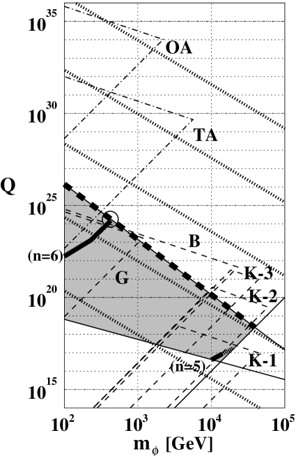
FIG. 12.: Summary of constraints on ($Q,m_{\phi}$) plain for the usual type of the Q ball. We also show the regions currently excluded by BAKSAN (B), Gyrlyand (G), and Kamiokande (K-1, K-2, K-3), and to be searched by the Telescope Array Project (TA) and OWL-AIRWATCH (OA) in the future. For the details of experiments, see Ref. [22]. Two thick lines within the shaded region denote the consistent scenarios for $n=5$ and $n=6$ cases, respectively, and the only allowed consistent scenario is found inside the circle. Five thick dotted lines denote the constraints of the dark matter Q ball which do not account for the baryogenesis for $T_{RH}=10^{2}$, $10^{3}$, $10^{4}$, $10^{5}$, and $10^{6}$ GeV from the top to the bottom.

As can be seen in Fig. 12, several experiments constrain the parameter space. The Q ball can be detected through so-called Kusenko-Kuzmin-Shaposhnikov-Tinyakov (KKST) process. When nucleons collide with a Q ball, they enter the surface layer of the Q ball, and dissociate into quarks, which are converted into squarks. In this process, Q balls release $\sim 1$ GeV energy per collision by emitting soft pions. This is the basis for the Q-ball detections [21, 22]. Lower left regions are excluded by the various experiments. The allowed charges are $Q\sim 10^{25}$ with $m_{\phi}=100$ GeV $-1$ TeV for $\varepsilon=1$, and future experiments such as the Telescope Array Project or the OWL-AIRWATCH detector may detect the dark matter Q balls.

We also put the consistent scenario in Fig. 12, which we considered in Sec. VII. Two thick lines inside the allowed region (shaded region) represent for the $n=5$ and $n=6$ cases. Hatched line connected to the thick line for $n=5$ shows the allowed region if we do not assume that the A terms come from the nonrenormalizable superpotential. The current experiments exclude the $n=5$ case, but the top edge of $n=6$ case is allowed, which we show by circle in the figure. Although the $n=6$ case sits at very interesting region, this dark matter Q ball may not be detected by future experiments as mentioned above.

If we do not impose the condition that the evaporated charges from Q balls account for the baryons in the universe, the only constraint is that the energy density of Q balls must not exceed the critical density. As mentioned in the previous section, this condition is Eq.(90):

$$Q\sim 9.3\times 10^{21} \varepsilon^{8/5}\Omega_{Q}^{12/5}\left(\frac{T_{RH}}{10^{5}{\rm GeV}}\right)^{-4}$$ (248)

$$\times\left(\frac{\beta}{6\times 10^{-4}}\right)^{8/5}\left(\frac{m_{\phi}}{\rm TeV}\right)^{-12/5}.$$

The Q-ball charge depends on the reheating temperature, and thick dotted parallel lines show the constraints for $T_{RH}=10^{2}$, $10^{3}$, $10^{4}$, $10^{5}$, and $10^{6}$ GeV from the top to the bottom in the figure. We can thus discover the dark matter Q balls in the future experiments, if the reheating temperature is low enough. Notice that the lower reheating temperature is favored by the supersymmetric models because of evading the cosmological gravitino problem [19].

B Q balls in the generic logarithmic potential

Now we show the allowed region for the Q-ball formation in the generic potential, but actual formation takes place when the thermal logarithmic term still dominates the potential. We show for the $n=6$ case, which is the only successful scenario in this situation, in Fig. 13. The thick solid line denotes the natural consistent scenario, while the thick dashed line represents the allowed region on the B-DM condition line in a more general situation that the Q-ball formation occurs through the different mechanism. On these lines, the Q balls can account for both the dark matter and the baryons in the universe simultaneously. Most of the parameter space is excluded by currents experiments, but very interesting region such as $Q\sim 10^{24}$ and $M_{F}\sim 5\times 10^{2}$ GeV is allowed. Notice that the dark matter Q balls with larger charges can be detected by the future experiments such as TA and OA, although they cannot play the role for the baryogenesis.

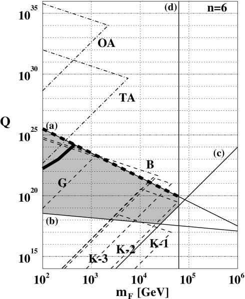
FIG. 13.: Summary of constraints on the parameter space ($Q,M_{F}$) with $n=6$ and $m_{\phi}=100$ GeV in the generic logarithmic potential where the thermal terms are dominated when the Q-ball formation occurs. Dashed and dot-dashed lines represent the same current and future experiments, respectively, as shown in Fig. 12. Lines (a), (b), and (c) denote the B-DM, survival, and stability conditions, respectively. Line (d) shows the conditions $T\gtrsim M_{F}$. Notice that this condition depends on $n$. The thick solid line is the allowed region of the successful scenario for the dark matter Q balls supplying the baryons in the universe, while the thick dashed line represents more general cases.

C Q balls in the gravity-mediation dominated potential

Next, we move on to the ‘new’ type of Q ball. The constraints on parameter space $(Q,m_{3/2})$ were obtained in Ref. [6]. Here we only draw the results. The regions where both the amount of the baryon and the dark matter can be explained are shown as thick lines in Fig. 14. Lower left regions are excluded by the various experiments. Notice that future experiments such as the Telescope Array Project or the OWL-AIRWATCH detector may detect this type of the dark matter Q balls, supplying the baryons in the universe, with an interesting gravitino mass $\sim 100$ keV, if the the origin of the A terms differs from the nonrenormalizable superpotential.

FIG. 14.: Restrictions by several experiments on ($Q,m_{3/2}$) plain for $|K|=0.01$. We show the regions currently excluded by BAKSAN (B), Gyrlyand (G), and Kamiokande (K-1, K-2, K-3), and to be searched by the Telescope Array Project (TA) and OWL-AIRWATCH (OA) in the future. The thick lines represent for the gravity-mediation type of the Q ball to be both the dark matter and the source for the baryons of the universe for $m_{\phi}=300$ GeV, 1 TeV, and 3 TeV from the top to the bottom. Three dot-dashed lines denote the constraints of the dark matter Q ball which do not account for the baryogenesis for $T_{RH}=10^{3}$, $10^{5}$, and $10^{7}$ GeV from the top to the bottom.

Although any consistent cosmological Q-ball scenario does not exist in the framework that both the initial amplitude and the A terms of the AD field are determined by the nonrenormalizable superpotential, it is not necessarily true that the dark matter Q balls do not exist whether they can be the source for the baryons in the universe or not. In general, we have the constraint for the Q balls to be a crucial component of the dark matter. It reads as

$$Q\sim 3.5\times 10^{26}\Omega_{Q}\left(\frac{\beta}{6\times 10^{-4}}\right)\left(\frac{m_{3/2}}{\rm MeV}\right)^{-2}\left(\frac{T_{RH}}{10^{5}{\rm GeV}}\right)^{-1},$$ (249)

where Eq.(151) is used.

Three dot-dashed lines are shown for $T_{RH}=10^{3}$, $10^{5}$, and $10^{7}$, from the top to the bottom, respectively. Therefore, the dark matter Q balls can be detected in the future experiments for the low reheating temperature universe, which is free from the cosmological gravitino problem. Notice that the baryons have to be supplied by another mechanism in this case.

D Delayed Q balls in the thermal logarithmic potential

As shown in the previous sections, we can restrict the parameter space $(Q,M_{F})$ by several conditions for the Q-ball formation in the natural scenarios. In general, we have three conditions: the B-DM, survival, and stability conditions. Here, we write them down again:

$${\rm(a)}\quad Q \sim 3.2\times 10^{17}\varepsilon^{3/2}\Omega_{Q}^{3/2}\eta_{B,10}^{-3/2}m_{\phi,2}^{-1}M_{F,6}^{-2},$$ (250)

$${\rm(b)}\quad Q \gtrsim 1.2\times 10^{17}m_{\phi,2}^{-8/11}M_{F,6}^{-4/11},$$ (251)

$${\rm(c)}\quad Q \gtrsim 10^{24}M_{F,6}^{4}.$$ (252)

We plot these lines in Figs. 15 and 16 for $n=6$ and $n=7$ cases, respectively. In these figures, (a), (b), and (c) denote the B-DM, survival, and stability conditions, respectively, for $\Omega_{Q}=1$ and $m_{\phi}=100$ GeV. We also show the data from several experiments. These are the same as we have used above. The experimental lines are the same as that for the specific logarithmic potential, if we just replace $m_{\phi}$ by $M_{F}$. We plot these data, using the fact that the flux is related to the Q-ball mass, and the cross section is related to the Q-ball size. Therefore, these Q-ball parameters can be expressed in the same form as in the specific potential for the replacement of $m_{\phi}$ by $M_{F}$ in the generic potential. Notice that the presence of the dark matter Q balls for $m_{\phi}=1$ TeV is almost excluded by experiments: Only Q balls with $Q\simeq 10^{19}$ and $M_{F}\simeq 5.6\times 10^{4}$ GeV are allowed.

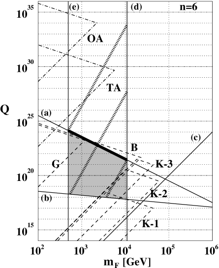
FIG. 15.: Summary of constraints on the parameter space $(Q,M_{F})$ for the delayed-formed Q balls with the thermal logarithmic term domination for $m_{\phi}=100$ GeV and $n=6$. Dashed and dot-dashed lines represent the same current and future experiments, respectively, as shown in Fig. 12. Lines (a), (b), and (c) denote the B-DM, survival, and stability conditions, respectively. Lines (d) and (e) show the conditions $T_{eq}\gtrsim M_{F}$ and $m_{3/2}\lesssim 1$ GeV, respectively. The thick solid line is the allowed region of the successful scenario for the dark matter Q balls supplying the baryons in the universe. Thick dotted lines denote the formed Q-ball charges with $T_{RH}\sim 10^{7}$, $10^{3}$, and $29$ GeV from the top to the bottom.

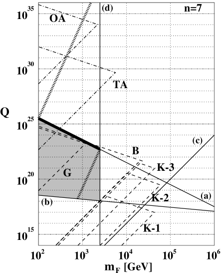
FIG. 16.: Summary of constraints on the parameter space $(Q,M_{F})$ for the delayed-formed Q balls with the thermal logarithmic term domination for $m_{\phi}=100$ GeV and $n=7$. Dashed and dot-dashed lines represent the same current and future experiments, respectively, as shown in Fig. 12. Lines (a), (b), and (c) denote the B-DM, survival, and stability conditions, respectively. Line (d) shows the condition $T_{RH}\gtrsim 10$ MeV. The thick solid line is the allowed region of the successful scenario for the dark matter Q balls supplying the baryons in the universe. Thick dotted lines denote the formed Q-ball charges with $T_{RH}\sim 62$ GeV and $10$ MeV for the upper and lower lines, respectively.

Now we put the conditions for the Q-ball formation to take place in the natural scenarios. In Fig. 15, vertical line (d) denotes for the condition that the thermal logarithmic potential dominates over the generic ones, i.e., $T_{eq}\gtrsim M_{F}$. Another vertical line (e) represents for $m_{3/2}\lesssim 1$ GeV in the gauge-mediated SUSY breaking model. Three thick dotted lines show the charges of the produced Q balls in the natural scenarios with the reheating temperature $1.0\times 10^{7}$, $1.0\times 10^{3}$, and $29$ GeV from the top to the bottom, respectively. The thick solid line is the final answer, which represents the dark matter Q balls supplying the baryons in the universe in the natural scenario. Two remarks are following. (1) Those dark matter Q balls which do not account for the baryogenesis may be detected by the Telescope Array Project (TA), if their charges are $\sim 10^{29}$ and the reheating temperature is $\sim 10^{7}$ GeV. (2) There is no cosmological gravitino problem for this scenario.

In Fig. 16, line (d) denotes the condition that the reheating temperature should be higher than $10$ MeV in order for the nucleosynthesis to take place successfully. We also assume $M_{F}\gtrsim 100$ GeV. Two thick dotted lines represent the Q-ball charges from the formation mechanism with the reheating temperature 62 GeV and 10 MeV for upper and lower lines, respectively. Thick solid line shows the successful region that the Q balls account for both the dark matter and the source for the baryons in the universe simultaneously. Most of this region is allowed experimentally, and, in particular, the dark matter Q balls with $Q\sim 10^{25}$ may be detected by the TA in the future. Notice again that cosmological gravitino problem is avoided for such low reheating temperature.

Now we will mention the specific logarithmic potential, where $M_{F}=m_{\phi}$. We impose three general conditions; namely, the B-DM, survival, and stability conditions. They are written as [cf. Eqs.(245), (244), and (246)]

$${\rm(a)}\quad Q \sim 1.2\times 10^{23}\varepsilon^{3/2}\Omega_{Q}^{3/2}\eta_{B,10}^{-3/2}m_{\phi,{\rm TeV}}^{-3},$$ (253)

$${\rm(b)}\quad Q \gtrsim 7.4\times 10^{17}m_{\phi,{\rm TeV}}^{-12/11},$$ (254)

$${\rm(c)}\quad Q \gtrsim 10^{12}m_{\phi,{\rm TeV}}^{4},$$ (255)

which are shown in Figs. 17 and 18.

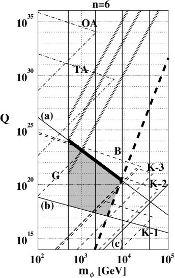
FIG. 17.: Summary of constraints on the parameter space $(Q,m_{\phi})$ for the delayed-formed Q balls with the thermal logarithmic term domination for $n=6$. Experimental lines are the same. Lines (a), (b), and (c) denote the B-DM, survival, and stability conditions, respectively. Thick dotted lines denote the formed Q-ball charges for $T_{RH}\simeq 10^{5}$, $3\times 10^{4}$, and $5\times 10^{3}$ GeV from the top to the bottom. The thick dashed line represents the condition $T_{eq}\gtrsim m_{\phi}$. The thick solid line is the allowed region of the successful scenario for the dark matter Q balls supplying the baryons in the universe. Solid vertical lines denote the gravitino mass ranges, $m_{3/2}=1$ GeV, 100 MeV, 10 MeV, and 1 MeV from the left to the right.

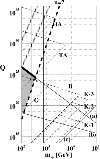
FIG. 18.: Summary of constraints on the parameter space $(Q,m_{\phi})$ for the delayed-formed Q balls with the thermal logarithmic term domination for $n=7$. Experimental lines are the same. Lines (a), (b), and (c) denote the B-DM, survival, and stability conditions, respectively. Thick dotted lines denote the formed Q-ball charges for $T_{RH}\simeq 10^{3}$ and $80$ GeV for the upper and lower lines. The thick dashed line represents the condition $T_{eq}\gtrsim m_{\phi}$. The thick solid line is the allowed region of the successful scenario for the dark matter Q balls supplying the baryons in the universe. Solid vertical lines denote the gravitino mass ranges, $m_{3/2}=100$ keV (left) and 10 keV (right).

The charge of the formed Q-ball and the initial amplitude of the field are expressed as

$$Q \sim 1.7\times 10^{26}\Omega_{Q}^{4/5}\beta_{\ell}^{4/5}m_{\phi,{\rm TeV}}^{4/5}T_{RH,5}^{4}m_{3/2,{\rm GeV}}^{-4},$$ (256)

$$\phi_{0} \sim 5.3\times 10^{14}\Omega_{Q}^{-2/5}\beta_{\ell}^{-1/10}$$ (258)

$$\hskip 42.67912pt\times m_{\phi,{\rm TeV}}^{2/5}T_{RH,5}^{2}m_{3/2,{\rm GeV}}^{-1}{\rm GeV},$$

respectively. The initial amplitude is determined by the balance between the Hubble mass and nonrenormalizable terms, and combining it with Eq.(258), we get the relation between $m_{\phi}$ and $m_{3/2}$ as

$$m_{\phi}\sim 4.9\times 10^{2}\Omega_{Q}\beta_{\ell}^{1/4}m_{3/2,{\rm GeV}}^{-5/8}\ {\rm GeV},$$ (259)

for $n=6$. We thus get the charge of the produced Q balls:

$$Q\sim 1.9\times 10^{28}\Omega_{Q}^{-28/5}\beta_{\ell}^{-4/5}T_{RH,5}^{4}m_{\phi,{\rm TeV}}^{36/5},$$ (260)

which we plot for $T_{RH}=10^{5}$, $3\times 10^{4}$, and $5\times 10^{3}$ GeV from the top to the bottom by thick dotted lines in Fig. 17. In order for this situation to take place, $T_{eq}\gtrsim m_{\phi}$, which leads to the constraint for the reheating temperature in terms of $m_{\phi}$ as

$$T_{RH}\gtrsim 4.4\Omega_{Q}^{1/5}\beta_{\ell}^{1/20}m_{\phi,{\rm TeV}}^{4/5}\ {\rm GeV}.$$ (261)

Inserting this constraint into Eq.(256), we have

$$Q\gtrsim 6.8\times 10^{10}\Omega_{Q}^{-24/5}\beta_{\ell}^{-3/5}m_{\phi,{\rm TeV}}^{52/5},$$ (262)

which is shown by the thick dashed line in Fig. 17. As is seen in the figure, the experimentally allowed region is very narrow, and the consistent natural scenario will work only for $Q\sim 10^{24}$, $m_{\phi}\sim 5\times 10^{2}$ GeV, $m_{3/2}\sim 1$ GeV, and $T_{RH}\sim 3\times 10^{4}$ GeV. Notice that there is no cosmological gravitino problem also in this case.

On the other hand, the relation between $m_{\phi}$ and $m_{3/2}$, which is obtained by equating Eq.(258) and the value determined by the balance between the Hubble mass and the nonrenormalizable term, is written as

$$m_{\phi}\sim 2.4\Omega_{Q}\beta_{\ell}^{1/4}m_{3/2,{\rm GeV}}^{-1/2}\ {\rm GeV},$$ (263)

for $n=7$. We thus get the charge of the produced Q balls:

$$Q\sim 1.9\times 10^{28}\Omega_{Q}^{-28/5}\beta_{\ell}^{-4/5}T_{RH,5}^{4}m_{\phi,{\rm TeV}}^{36/5},$$ (264)

where we plot for $T_{RH}=10^{3}$ and 80 GeV for the upper and the lower thick dotted lines, respectively, in Fig. 18. Taking into account the condition $T_{eq}\gtrsim m_{\phi}$, we obtain

$$Q\gtrsim 6.1\times 10^{29}\Omega_{Q}^{-32/5}\beta_{\ell}^{-1}m_{\phi,{\rm TeV}}^{12},$$ (265)

where Eq.(261) is used. We plot this constraint by the thick dashed line in Fig. 18. The allowed region for the dark matter Q balls, which are also the source for the baryons in the universe, is shown by thick solid line. This region does not suffer from the current experimental limit and this dark matter Q ball with $Q\sim 10^{25}$ and $m_{3/2}\sim 100$ keV may be detected by TA in the future. Notice that the reheating temperature is low enough to avoid the cosmological gravitino problem. If we abandon to explain the baryons in the universe by the charge evaporation from Q balls, the dark matter Q balls may be found by TA and also OWL-AIRWATCH in the future.

E Delayed Q balls in the generic logarithmic potential

As mentioned in the previous section, we have obtained the consistent scenarios of the dark matter Q ball explaining the baryons of the universe naturally, with the initial conditions determined by the balance of the Hubble and the nonrenormalizable terms in the effective potential, with $n=6$, 7, and 8. However, the parameter space is restricted by the current experiments. We plot the allowed regions and experimentally excluded regions for $n=6$, 7, and 8 in Figs. 19, 20, and 21, respectively. In these figures, lines (a), (b), and (c) are the B-DM, survival, and stability conditions, respectively. Lines (d) in Figs. 19 and 20 are the condition $M_{F}\gtrsim T_{eq}$, while $T_{RH}\gtrsim 10$ MeV is shown as line (d) in Fig. 21. Lines (e) in Figs. 19 and 20 are just the upper limit for $M_{F}$.

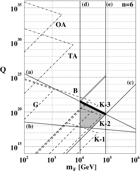
FIG. 19.: Summary of constraints on the parameter space $(Q,M_{F})$ for the delayed-formed Q balls with the generic logarithmic term domination for $n=6$ and $m_{\phi}=100$ GeV. Experimental lines are the same. Lines (a), (b), and (c) denote the B-DM, survival, and stability conditions, respectively. Line (d) represents the condition $M_{F}\gtrsim T_{eq}$, and line (e) is just the upper limit for $M_{F}$.

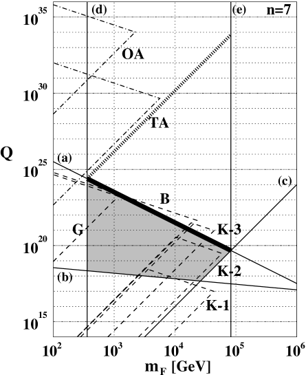
FIG. 20.: Summary of constraints on the parameter space $(Q,M_{F})$ for the delayed-formed Q balls with the generic logarithmic term domination for $n=7$ and $m_{\phi}=100$ GeV. Experimental lines are the same. Lines (a), (b), and (c) denote the B-DM, survival, and stability conditions, respectively. Line (d) represents the condition $M_{F}\gtrsim T_{eq}$, and line (e) is just the upper limit for $M_{F}$.

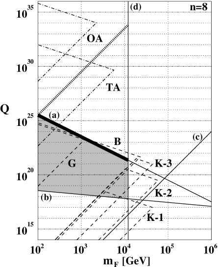
FIG. 21.: Summary of constraints on the parameter space $(Q,M_{F})$ for the delayed-formed Q balls with the generic logarithmic term domination for $n=8$ and $m_{\phi}=100$ GeV. Experimental lines are the same. Lines (a), (b), and (c) denote the B-DM, survival, and stability conditions, respectively. Line (d) represents the condition $T_{RH}\gtrsim 10$ MeV.

We can see some parameter regions which are experimentally allowed in each figures. Typically, there are two types: One is for $Q\sim 10^{20}$ and $M_{F}\sim 5\times 10^{4}$ GeV, and the other is for $Q\sim 10^{25}$ and $M_{F}\sim 3\times 10^{2}$ GeV. In the latter case, the dark matter Q balls may be detected in the future experiments. Notice that the required reheating temperature is rather too low (100 MeV $-$ 10 GeV), which is very difficult to realize in the actual inflation model.

XI Conclusion

We have investigated thoroughly the Q-ball cosmology (the baryogenesis and the dark matter) in the gauge-mediated SUSY breaking model. Taking into account thermal effects, the shape of the effective potential has to be altered somewhat, but most of the features of the Q-ball formation derived at zero temperature can be applied to the finite temperature case with appropriate rescalings. We have thus found that Q balls are actually formed through Affleck-Dine mechanism in the early universe.

We have sought for the consistent scenario for the dark matter Q ball, which also provides the baryon number of the universe simultaneously. For the consistent scenario, we adopt the nonrenormalizable superpotential in order to naturally give the initial amplitude of the AD field and the source for the field rotation due to the A-term. As opposed to our expectation, very narrow parameter region could be useful for the scenario in the situations that the Q balls are produced just after the baryon number creation. In addition, we have seen that current experiments have already excluded most of the successful parameter regions.

Of course, if the A-terms and/or the initial amplitude of the AD field are determined by other mechanism, the cosmological Q-ball scenario may work. Then, the stable dark matter Q balls supplying the baryons play a crucial role in the universe.

We have also found the new situations that the Q-ball formation takes place when the amplitude of the fields becomes small enough to be in the logarithmic terms in the potential, while the fields starts its rotation at larger amplitudes where the effective potential is dominated by the gravity-mediation term with positive K-term. This allows to produce Q balls with smaller charges while creating larger baryon numbers. In this situation, there is wider allowed regions for naturally consistent scenario, although the current experiments exclude most of the parameter space. Notice also that rather too low reheating temperature is necessary for larger $n$ scenario to work naturally. This aspect is good for evading the cosmological gravitino problem, while it is difficult to construct the actual inflation mechanism to get such low reheating temperatures, in spite of the fact that the nucleosynthesis can take place successfully for the reheating temperature higher than at least 10 MeV.

So far we have investigated the possibility that the dark matter Q balls which supply the baryon number of the universe could be really produced in the naturally consistent scenario, where the initial amplitude of the AD field and the A terms for the field rotation are determined by the nonrenormalizable superpotential. Here, we have explicitly imposed that the produced Q balls must be stable against the decay into nucleons in order for Q balls themselves to be the dark matter of the universe. However, there may be such situations that Q balls decay into lighter particles when the stability condition is broken. This situation is almost the same as the usual AD baryogenesis when we consider only the baryons in the universe. Moreover, if the decay products include the lightest supersymmetric particles (LSPs), they may account for the dark matter of the universe.

If this is the case, gravitino may be the LSP to be the dark matter. The number density of LSP depends on the lifetime of the Q ball, as investigated in Ref. [13] for the gravity-mediated SUSY breaking model. If it decays before the temperature drops the freeze-out temperature of LSPs, the density follows the thermal value. On the other hand, when its lifetime is long enough, the ratio of the number of the baryons to that of LSPs is fixed, and we can directly estimate the relation between the amounts of the baryons and the LSP dark matter of the universe.

REFERENCES

• [1] I. Affleck and M. Dine, Nucl. Phys. B249, 361 (1985).
• [2] A. Kusenko and M. Shaposhnikov, Phys. Lett. B418, 46 (1998).
• [3] S. Coleman, Nucl. Phys. B262, 263 (1985).
• [4] S. Kasuya and M. Kawasaki, Phys. Rev. D61, 041301 (2000).
• [5] M. Laine and M. Shaposhnikov, Nucl. Phys. B532, 376 (1998).
• [6] S. Kasuya and M. Kawasaki, Phys. Rev. Lett. 85, 2677 (2000).
• [7] M. Dine, L. Randall, and S. Thomas, Nucl. Phys. B458, 291 (1996).
• [8] T. Gherghetta, C. Kolda, and S.P. Martin, Nucl. Phys. B468, 37 (1996).
• [9] A. de Gouvêa, T. Moroi, and H. Murayama, Phys. Rev. D56, 1281 (1997).
• [10] K. Enqvist and J. McDonald, Phys. Lett. B425, 309 (1998).
• [11] A. Anisimov and M. Dine, hep-ph/0008058, 2000.
• [12] M. Fujii, K. Hamaguchi, and T. Yanagida, Phys. Rev. 63, 123513 (2001).
• [13] K. Enqvist and J. McDonald, Nucl. Phys. B538, 321 (1999).
• [14] S. Kasuya and M. Kawasaki, Phys. Rev. D62, 023512 (2000).
• [15] S. Kasuya, in Proceedings of the 7th International Symposium on Particles, Strings and Cosmology (PASCOS-99), 1999, Lake Tahoe, California, USA, pp. 301-304.
• [16] K. Enqvist, A. Jokinen, and J. McDonald, Phys. Lett. B483, 191 (2000).
• [17] R. Banerjee and K. Jedamzik, Phys. Lett. B484, 278 (2000).
• [18] S. Kasuya, in Proceedings of the 4th International Workshop on Particle Physics and the Early Universe (COSMO-2000), 2000, Cheju, South Korea.
• [19] T. Moroi, Ph.D. thesis, Tohoku University, hep-ph/9503210, 1995.
• [20] M. Kawasaki, K. Kohri, and N. Sugiyama, Phys. Rev. D62, 023506 (2000).
• [21] A. Kusenko, V. Kuzmin, M. Shaposhnikov, and P.G. Tinyakov, Phys. Rev. Lett. 80, 3185 (1998).
• [22] J. Arafune, T. Yoshida, S. Nakamura, and K. Ogure, Phys. Rev. D62, 105013 (2000), and references therein.