Next-to-leading order evolution of generalized parton distributions for DESY HERA and HERMES

Abstract

The QCD evolution of both unpolarized and polarized generalized parton distributions (GPDs) to next-to-leading order (NLO) accuracy is presented, in both the DGLAP and ERBL regions, for two appropriately symmetrized input distributions based on conventional parton density functions. To illustrate the relative size of the NLO corrections a comparison is made with leading order evolution of the same distributions. For the first time, NLO results are given for both small and large values of the skewedness parameter, $\zeta=x_{bj}$, i.e. for all of the kinematic range relevant to HERA and HERMES.

I Introduction

Generalized Partons Distributions (GPDs) [1, 2, 3, 4] are generic two-parton correlation functions of nucleons that provide the boundary conditions for the calculation of various hard, exclusive, diffractive processes in QCD. For such processes, which are characterised by a suitable hard scale (for example a large photon virtuality, $Q^{2}$, in Deep Inelastic Scattering (DIS) experiments), the incoming nucleon remains intact and at high energies is well separated in rapidity from the rest of the final state, i. e. the diffractively produced low mass particle (e.g. a meson or real photon). A perturbative QCD analysis is possible provided that a factorization theorem is proved which illustrates the separation of short and long distance physics. The QCD amplitude is then a sum of terms involving a convolution of a hard scattering coefficient (calculated to a given order in $\alpha_{s}$) with a GPD (specified to a related accuracy in logarithms) and possibly a second convolution with a distribution amplitude, in the case of the production of a hadronic final state.

The universal, non-perturbative GPDs obey renormalization group equations (RGE) and are formally defined, up to power suppressed contributions, by Fourier transforms of non-local, renormalized, light-cone operators sandwiched between nucleon states of unequal momentum (the corresponding distributions in inclusive DIS involve equal momenta for the incoming and outgoing nucleon). In common with conventional DGLAP parton distribution functions, GPDs cannot be calculated from first principles at present due to the confinement problem, but they can be pinned down through a global RGE analysis of all available experimental data. The simplest example of such a hard, exclusive, diffractive process is deeply virtual Compton scattering (DVCS) [1, 2, 5, 6], for which there is recent first data available from HERA [7, 8], HERMES [9] and JLAB [10].

The RGE for the GPDs involve kernels which have been computed up to next-to-leading order (NLO) in perturbation theory so far [11]. The solutions of these NLO evolution equations are necessary to obtain accurate predictions for various experimentally accessible processes. In fact the DVCS amplitude itself can be directly accessed experimentally through the interference of DVCS with the Bethe-Heitler process [7, 8, 9]. In this paper we present numerical solutions to the NLO QCD evolution of the GPDs for large (HERMES) and small (HERA) skewedness which corresponds to large and small Bjorken $x$ in the particular representation used. As input for the NLO evolution, we use a model based on double distributions (DDs) [12, 13] incorporating for comparison two related sets of conventional NLO unpolarized and polarized parton distribution functions (PDFs), MRSA${}^{{}^{\prime}}$ [14] and Gehrmann-Stirling (‘GS(A)’)[15], and GRV98 [16] and GRSV00 [17], respectively. The resultant input GPDs, by design, respect all the known symmetries and properties of the GPDs, which are preserved under evolution. This latter condition constitutes a stringent test of any proposed solutions, which is passed by our numerical solutions to very good accuracy.

This paper presents the first results of the numerical solution to the RGEs at NLO accuracy [18, 19, 20] for any $x$ (see, e.g., [21, 22] for leading order skewed evolution) and is organised as follows. In section II we give the formal definitions of the GPDs and discuss their symmetry and spectral properties. Section III describes our choice of input distributions to the evolution equations outlined in section IV. We present our numerical results, including a comparison between leading order and next-to-leading order skewed evolution and a comparison with conventional next-to-leading order evolution, in section V, and conclude in section VI. Our evolution code will be made available to the community in the near future via the internet [23].

II Definitions, symmetries and spectral representations of GPDs

Amplitudes for quark and gluon correlators of unequal momentum nucleon states may be defined in a number of ways. We choose a definition which treats the initial and final state nucleon momentum ($p,p^{\prime}$, respectively) symmetrically by involving parton light-cone fractions with respect to the momentum transfer, $r=p-p^{\prime}$, and the average momentum, $\bar{P}=(p+p^{\prime})/2$. The flavour singlet and non-singlet (S,NS) quark, and the gluon (G) matrix elements of the non-local operators, involving a light-cone vector $z^{\mu}$ ($z^{2}=0$), are defined by

$$2M_{a}^{NS}(\bar{P}\cdot z,r\cdot z,t)=$$ (1)

$$\langle N\left(P_{-}\right)|{\bar{\psi}}_{a}\left(-\frac{z}{2}\right){\cal P}\hat{z}\psi_{a}\left(\frac{z}{2}\right)|N\left(P_{+}\right)\rangle+$$ (2)

$$\langle N\left(P_{-}\right)|{\bar{\psi}}_{a}\left(\frac{z}{2}\right){\cal P}\hat{z}\psi_{a}\left(-\frac{z}{2}\right)|N\left(P_{+}\right)\rangle\,,$$ (3)

$$2M^{S}(\bar{P}\cdot z,r\cdot z,t)=$$ (4)

$$\sum_{a}\langle N\left(P_{-}\right)|{\bar{\psi}}_{a}\left(-\frac{z}{2}\right){\cal P}\hat{z}\psi_{a}\left(\frac{z}{2}\right)|N\left(P_{+}\right)\rangle-$$ (5)

$$\langle N\left(P_{-}\right)|{\bar{\psi}}_{a}\left(\frac{z}{2}\right){\cal P}\hat{z}\psi_{a}\left(-\frac{z}{2}\right)|N\left(P_{+}\right)\rangle\,,$$ (6)

$$2M^{G}(\bar{P}\cdot z,r\cdot z,t)=$$ (7)

$$z^{\mu}z^{\nu}\langle N\left(P_{-}\right)|G_{\mu\rho}\left(-\frac{z}{2}\right){\cal P}G^{\rho}_{\nu}\left(\frac{z}{2}\right)|N\left(P_{+}\right)\rangle+$$ (8)

$$z^{\mu}z^{\nu}\langle N\left(P_{-}\right)|G_{\mu\rho}\left(\frac{z}{2}\right){\cal P}G^{\rho}_{\nu}\left(-\frac{z}{2}\right)|N\left(P_{+}\right)\rangle,$$ (9)

where $P_{+,-}=\bar{P}\pm\frac{r}{2}$, $t=r^{2}$ is the four-momentum transfer, ${\hat{z}}=\gamma^{\mu}z_{\mu}$, $\bar{P}\cdot z$ and $r\cdot z$ are dimensionless Lorentz scalars, $a=u,d,s,c...$ is a flavour index and the symbol $\cal P$ represents the usual path ordered exponential. The spin and isospin dependence have been suppressed for convenience. Polarized matrix elements are defined in a similar fashion, but with $\hat{z}\to\hat{z}\gamma^{5}$ for the quark and with the implicit metric $g^{\mu\nu}\to i\epsilon^{\mu\nu-+}$ for the gluon. The unpolarized matrix elements, and thus their associated GPDs, have definite symmetry properties. G-parity gives (suppressing the $t$-dependence)

$$M^{NS}(\bar{P}\cdot z,r\cdot z)=-M^{NS}(-\bar{P}\cdot z,-r\cdot z)$$ (11)

$$M^{S,G}(\bar{P}\cdot z,r\cdot z)=M^{S,G}(-\bar{P}\cdot z,-r\cdot z)\,.$$ (12)

The opposite properties are observed for the polarized case. Hermitian conjugation gives for all polarized and unpolarized species ($i=S,NS,G$)

$$M^{i}(\bar{P}\cdot z,r\cdot z)=M^{i}(\bar{P}\cdot z,-r\cdot z)\,.$$ (13)

The matrix elements can be most generally represented by a double spectral representation with respect to $\bar{P}\cdot z$ and $r\cdot z$ [1, 3, 24] as follows:

$$M^{NS}=\int^{1}_{-1}dxe^{-ix\bar{P}\cdot z}\int^{1-|x|}_{-1+|x|}dye^{-iyr\cdot z/2}\times\,\,\,$$ (14)

$$\left[\bar{U}^{\prime}\hat{z}UF^{NS}(x,y,t)+\frac{iz^{\mu}r^{\nu}\bar{U}^{\prime}\sigma_{\mu\nu}U}{2m_{N}}K^{NS}(x,y,t)\right]\,,$$ (15)

$$M^{G}=\int^{1}_{-1}dxe^{-ix\bar{P}\cdot z}\int^{1-|x|}_{-1+|x|}dye^{-iyr\cdot z/2}\times$$ (16)

$$\Big{[}\bar{U}^{\prime}\hat{z}U\frac{\bar{P}\cdot z}{2}F^{G}(x,y,t)\,$$ (17)

$$+\frac{iz^{\mu}r^{\nu}\bar{U}^{\prime}\sigma_{\mu\nu}Ur\cdot z}{4m_{N}}K^{G}(x,y,t)\Big{]}$$ (18)

$$+{\bar{U}^{\prime}}Ur\cdot z\int^{1}_{-1}dye^{-iyr\cdot z/2}D^{G}(y,t)\,,$$ (19)

$$M^{S}=\int^{1}_{-1}dxe^{-ix\bar{P}\cdot z}\int^{1-|x|}_{-1+|x|}dye^{-iyr\cdot z/2}\times$$ (20)

$$\left[\bar{U}^{\prime}\hat{z}UF^{S}(x,y,t)+\frac{iz^{\mu}r^{\nu}\bar{U}^{\prime}\sigma_{\mu\nu}U}{2m_{N}}K^{S}(x,y,t)\right]$$ (21)

$$+{\bar{U}^{\prime}}Ur\cdot z\int^{1}_{-1}dye^{-iyr\cdot z/2}D(y,t)\,,$$ (22)

where $\bar{U}^{{}^{\prime}}$ and $U$ are nucleon spinors. Note that in accordance with the associated Lorentz structures, the $F$’s correspond to helicity non-flip and the $K$’s to helicity flip amplitudes, and are collectively known as double distributions. Henceforth, for brevity, we shall only discuss the helicity non-flip piece explicitly. However, the helicity flip case is exactly analogous. The $D$-terms in the last two lines permit non-zero values for the singlet $M^{S}$ and $M^{G}$ in the limit $\bar{P}\cdot z\to 0$ and $r\cdot z\neq 0$, which is allowed by their evenness in $\bar{P}\cdot z$ (cf. eq.(12)). Conversely, $M^{NS}$ is required by its oddness under $\bar{P}\cdot z$, for any $r\cdot z$, to be zero [24].

By making a particular choice of the light-cone vector, $z^{\mu}$, as a light-ray vector (so that in light-cone variables, $z_{\pm}=z_{0}\pm z_{3}$, only its minus component is non-zero $z^{\mu}=(0,z_{-},0)$) one may reduce the double spectral representation of eq.(22), defined on the entire light-cone, to a one dimensional spectral representation, defined along a light ray, depending on the skewedness parameter, $\xi$, defined by

$$\xi=r\cdot z/2\bar{P}\cdot z=r_{+}/2{\bar{P}}_{+}\,.$$ (23)

The resultant GPDs are the off-forward distribution functions (OFPDFs) introduced in [1, 2]:

$$H(v,\xi,t)=$$ (24)

$$\int^{1}_{-1}dx^{\prime}\int^{1-|x^{\prime}|}_{-1+|x^{\prime}|}dy^{\prime}\delta(x^{\prime}+\xi y^{\prime}-v)F(x^{\prime},y^{\prime},t)\,,$$ (25)

where $v\in[-1,1]$. In terms of individual flavour decomposition the singlet, non-singlet and gluon distributions are given through

$$H^{S}(v,\xi)=\sum_{a}H^{q,a}(v,\xi)\mp H^{q,a}(-v,\xi)\,,$$ (26)

$$H^{NS,a}(v,\xi)=H^{q,a}(v,\xi)\pm H^{q,a}(-v,\xi)\,,$$ (27)

$$H^{G}(v,\xi)=H^{g}(v,\xi)\pm H^{g}(-v,\xi)\,,$$ (28)

where the upper (lower) signs corresponds to the unpolarized (polarized) case. The unpolarized singlet and the gluon have additional resonance-like contributions called the D-term [24, 25] which ensures the correct symmetry and polynomiality properties (cf. eq.(22)). Note that the symmetries which hold for the matrix elements change for the $H^{i}$s, due to the $\bar{P}\cdot z$, $\hat{z}$ factors in eq.(22). The unpolarized quark singlet is antisymmetric about $v=0$, whereas the unpolarized quark non-singlet and the gluon are symmetric. The opposite symmetries hold for the polarized distributions. The helicity flip GPDs, (labelled with $E$s), are found analogously (double integrals with respect to the $K$s).

Henceforth, we shall make the usual assumption that the $t$-dependence of all of these functions factorizes into implicit form factors. One should bear in mind that in order to make predictions for physical amplitudes (for $t\neq 0$) these form factors must be specified. Note that the assumption of a factorized $t$-dependence, as a general statement, must be justified within the kinematic regime concerned. It appears to be valid at small $x$ and small $t$, from the HERA data on a variety of diffractive measurements. However, it appears to be wrong for moderate to large $t$ and larger $x$ [26]. The evolution used in this note assumes the same factorized $t$-dependence for each parton species, which therefore factorizes in the evolution equations. Thus any effect of assuming a different $t$-dependence for quark singlet and gluon, which mix under evolution, is neglected (but could in principle be investigated within the same framework). The effect on evolution of relaxing the assumption of factorization of the $t$-dependence altogether remains an open question.

Taking the $N-1$ moments (for even $N$) of the GPDs yields a sum of polynomials in the skewedness parameter $\xi$ [24]:

$$\int^{1}_{-1}dvv^{N-1}H(v,\xi,t)=$$ (29)

$$\sum^{N}_{k=0}\xi^{k}\left(N\atop k\right)\int^{1}_{-1}dx\int^{1-|x|}_{-1+|x|}F(x,y,t)x^{N-k}y^{k}\,.$$ (30)

This powerful polynomiality condition arises because $\mu_{i}$ indices of a local operator $O^{\mu_{1}...\mu_{N}}$ must be carried by either ${\bar{P}}$ or $r$ (taking moments is equivalent to going from non-local to local operators). In building models for GPDs, eq.(30) always has to be fulfilled and thus strongly constrains any model for the GPDs. We incorporate it in a natural way in building our input distributions in section III.

For the purposes of comparing to experiment it is natural to define GPDs in terms of momentum fractions, $X\in[0,1]$, of the incoming proton momentum, $p$, carried by the outgoing parton. To this end we adapt the notation and definitions of [22] introducing two non-diagonal parton distribution functions (NDPDFs), ${\cal F}^{q}$ and ${\cal F}^{\bar{q}}$, for flavour, $a$:

$${\cal F}^{q,a}\left(X_{1}=\frac{v_{1}+\xi}{1+\xi},\zeta\right)=\frac{H^{q,a}(v_{1},\xi)}{(1-\zeta/2)}\,,$$ (31)

$${\cal F}^{{\bar{q}},a}\left(X_{2}=\frac{\xi-v_{2}}{1+\xi},\zeta\right)=-\frac{H^{q,a}(v_{2},\xi)}{(1-\zeta/2)}\,,$$ (32)

where $v_{1}\in[-\xi,1],\,v_{2}\in[-1,\xi]$ (see fig.(4) of [22]), $\zeta\equiv r_{+}/p_{+}$ is the skewedness defined on the domain $\zeta\in[0,1]$ such that $\xi=\zeta/(2-\zeta)$ and $\zeta=x_{bj}$ for DVCS, up to terms of ${\cal O}(x_{bj}t/Q^{2})$. The inverse transformations between the $v$s and $X$s is:

$$v_{1}=\frac{X_{1}-\zeta/2}{1-\zeta/2} \,,\, v_{2}=\frac{\zeta/2-X_{2}}{1-\zeta/2}\,.$$ (33)

For the gluon one may use either transformation, e.g.

$${\cal F}^{g}(X,\zeta) = \frac{H^{g}(v_{1},\xi)}{(1-\zeta/2)}\,.$$ (34)

There are two distinct kinematic regions for the GPDs, with different physical interpretations. In the DGLAP [27] region, $X>\zeta$ ($|v|>\xi$), ${\cal F}^{q}(X,\zeta)$ and ${\cal F}^{\bar{q}}(X,\zeta)$ are independent functions, corresponding to quark or anti-quark fields leaving the nucleon with momentum fraction $X$ and returning with positive momentum fraction $X-\zeta$. As such they correspond to a generalization of regular DGLAP PDFs (which have equal outgoing and returning fractions). In the ERBL [28] region, $X<\zeta$ ($|v|<\xi$), both quark and anti-quark carry positive momentum fractions ($X,\zeta-X$) away from the nucleon in a meson-like configuration, and the GPDs behave like ERBL [28] distributional amplitudes characterising mesons. This implies that ${\cal F}^{q}$ and ${\cal F}^{\bar{q}}$ are not independent in the ERBL region, indeed a symmetry is observed: ${\cal F}^{q}(\zeta-X,\zeta)={\cal F}^{\bar{q}}(X,\zeta)$ (which directly reflects the symmetry of $H^{q}(v,\xi)$ about $v=0$). Similarly, the gluon distribution, ${\cal F}^{g}$, is DGLAP-like for $X>\zeta$ and ERBL-like for $X<\zeta$. This leads to unpolarized non-singlet, ${\cal F}^{NS,a}={\cal F}^{q,a}-{\cal F}^{{\bar{q}},a}$, and gluon GPDs which are symmetric, and a singlet quark distribution ${\cal F}^{S}=\sum_{a}{\cal F}^{q,a}+{\cal F}^{{\bar{q}},a}$ which is antisymmetric, about the point $X=\zeta/2$ in the ERBL region. Again the opposite symmetries hold for the polarized distributions.

III Input GPDs

In this section we describe how to build input distributions, ${\cal F}^{q,{\bar{q}},g}(X,\zeta,Q_{0})$, at the input scale, $Q_{0}$, with the correct symmetries and properties from conventional PDFs in the DGLAP region, for both the unpolarized and polarized cases. These input NDPDFs then serve as the boundary conditions for our numerical evolution.

Factoring out the overall $t$-dependence we have for the quark for example ($v_{1}>-\xi$):

$${\cal F}^{q,a}(X,\zeta)=\frac{H^{q,a}(v_{1},\xi)}{1-\zeta/2}=$$ (35)

$$\int^{1}_{-1}dx^{\prime}\int^{1-|x^{\prime}|}_{-1+|x^{\prime}|}dy^{\prime}\delta\left(x^{\prime}+\xi y^{\prime}-v_{1}\right)\frac{F^{q,a}(x^{\prime},y^{\prime})}{\left(1-\zeta/2\right)}\,.$$ (36)

Following [12, 13, 20] we employ a factorized ansatz which expresses the double distribution as a product of a profile function, $\pi^{i}$, and a conventional PDF, $f^{i}$, $(i=q,g$):

$$F^{q,a}(x^{\prime},y^{\prime}) = \pi^{q}(x^{\prime},y^{\prime})f^{q,a}(x^{\prime})$$ (37)

$$= \frac{3}{4}\frac{(1-|x^{\prime}|)^{2}-{y^{\prime}}^{2}}{(1-|x^{\prime}|)^{3}}f^{q,a}(x^{\prime})\,,$$ (38)

$$F^{g}(x^{\prime},y^{\prime}) = \pi^{g}(x^{\prime},y^{\prime})f^{g}(x^{\prime})$$ (39)

$$= \frac{15}{16}\frac{((1-|x^{\prime}|)^{2}-{y^{\prime}}^{2})^{2}}{(1-|x^{\prime}|)^{5}}f^{g}(x^{\prime})\,,$$ (40)

for quark of flavour $a$, where

$$f^{g}(x) = xg(x,Q_{0})\Theta(x)+|x|g(|x|,Q_{0})\Theta(-x)\,,$$ (41)

$$f^{q,a}(x) = q^{a}(x,Q_{0})\Theta(x)-(\bar{q}^{a})(|x|,Q_{0})\Theta(-x)\,.$$ (42)

The profile functions are chosen to guarantee the correct symmetry properties in the ERBL region and their normalization is specified by demanding that the conventional distributions are reproduced in the forward limit: e.g. ${\cal F}^{g}(X,\zeta\to 0)\to f^{g}(X)$. We have explicitly checked this forward limit for our input codes against independent codes for the conventional PDFs (see fig.(1) later).

So far, models for polarized distributions have been strongly based, for reasons of consistency, on closely associated models for unpolarized distributions. For this reason we choose as our inputs these closely related pairs of models. Unfortunately, the polarized set of distributions of Gehrmann and Stirling (‘GS(A)’) [15] is rather old now and is based on the MRSA${}^{{}^{\prime}}$ unpolarized set [14]. Our other set is the very recent GRSV set from 2000 [17] which is based on the 1998 unpolarized model by GRV [16] (we will denote these GRSV00 and GRV98 respectively [30]).

Having defined this model for the double distribution one may then perform the $y^{\prime}$-integration in eq.(36) using the delta function. This modifies the limits on the $x^{\prime}$ integration according to the region concerned: for the DGLAP region $X>\zeta$ one has:

$${\cal F}^{q,a}(X,\zeta)=$$ (43)

$$\frac{2}{\zeta}\int^{\frac{v_{1}+\xi}{1+\xi}}_{\frac{v_{1}-\xi}{1-\xi}}dx^{\prime}\pi^{q}\left(x^{\prime},\frac{v_{1}-x^{\prime}}{\xi}\right)q^{a}(x^{\prime})\,.$$ (44)

For the anti-quark, since $v_{2}=-v_{1}$ one may use eqs.(32,36) with $v_{2},v_{1}\to-v_{1}$, and exploiting the fact that $f^{q}(x)=-{\bar{q}}(|x|)$ for $x<0$, one arrives at

$${\cal F}^{\bar{q},a}(X,\zeta)=$$ (45)

$$\frac{2}{\zeta}\int^{\frac{-v_{1}+\xi}{1-\xi}}_{\frac{-v_{1}-\xi}{1+\xi}}dx^{\prime}\pi^{q}\left(x^{\prime},\frac{-v_{1}-x^{\prime}}{\xi}\right){\bar{q}}^{a}(|x^{\prime}|).$$ (46)

The non-singlet (valence) and singlet quark combinations are given by:

$${\cal F}^{NS,a} \equiv {\cal F}^{q,a}-{\cal F}^{{\bar{q}},a}$$ (47)

$$\equiv \frac{[H^{q,a}(v_{1},\xi)+H^{q,a}(-v_{1},\xi)]}{1-\zeta/2}\,,$$ (48)

$${\cal F}^{S} \equiv \sum_{a}{\cal F}^{q,a}+{\cal F}^{{\bar{q}},a}$$ (49)

$$\equiv \sum_{a}\frac{[H^{q,a}(v_{1},\xi)-H^{q,a}(-v_{1},\xi)]}{1-\zeta/2}\,.$$ (50)

In the ERBL region ($X>\zeta,|v|<\xi$) integration over $y^{\prime}$ leads to:

$${\cal F}^{q,a}(X,\zeta)=\frac{2}{\zeta}\times$$ (51)

$$\left[\int^{\frac{v_{1}+\xi}{1+\xi}}_{0}dx^{\prime}\pi^{q}\left(x^{\prime},\frac{v_{1}-x^{\prime}}{\xi}\right)q^{a}(x^{\prime})\,-\right.$$ (52)

$$\left.\int^{0}_{\frac{-(\xi-v_{1})}{1+\xi}}dx^{\prime}\pi^{q}\left(x^{\prime},\frac{v_{1}-x^{\prime}}{\xi}\right){\bar{q}}^{a}(|x^{\prime}|)\right]\,,$$ (53)

$${\cal F}^{{\bar{q}},a}(X,\zeta)=-\frac{2}{\zeta}\times$$ (54)

$$\left[\int^{\frac{\xi-v_{1}}{1+\xi}}_{0}dx^{\prime}\pi^{q}\left(x^{\prime},\frac{-v_{1}-x^{\prime}}{\xi}\right)q^{a}(x^{\prime})\,-\right.$$ (55)

$$\left.\int^{0}_{\frac{-(\xi+v_{1})}{1+\xi}}dx^{\prime}\pi^{q}\left(x^{\prime},\frac{-v_{1}-x^{\prime}}{\xi}\right){\bar{q}}^{a}(|x^{\prime}|)\right]\,.$$ (56)

This gives singlet and non-singlet distributions in the ERBL region containing four integrals over $x^{\prime}$. The unpolarized singlet also includes the D-term on the right hand side of eq.(50) (in principle there is also an analogous term in the unpolarized gluon ($D^{G}$ in eq.(22)), but we choose to set this to zero, since nothing is known for the gluon D-term except its symmetry.). We adapt the model introduced in [25] for the unpolarized singlet D-term based on the chiral-soliton model:

$${\cal F}^{D}(X,\zeta)=\Theta(\zeta-X)\,D\left(\frac{2X}{\zeta}-1,t=0\right)\,,$$ (57)

with $D$ given by a truncated expansion in terms of odd Gegenbauer Polynomials:

$$D(a)=(1-a^{2})\times$$ (58)

$$\left[-4.0C_{1}^{3/2}(a)-1.2C_{3}^{3/2}(a)-0.4C_{5}^{3/2}(a)\right]\,.$$ (59)

This D-term is antisymmetric in its argument, i. e. about the point $X=\zeta/2$ (in keeping with the anti-symmetry of ${\cal F}^{S}$, and $H^{S}$ about $v=0$). It vanishes entirely in the forward limit and only assumes numerical significance for large $\zeta$. This completes the definition of the input singlet and non-singlet quark distributions in both regions. The input gluon is defined along the same lines as the non-singlet.

IV NLO evolution of GPDs

The input GPDs, defined above, are continuous functions which span the DGLAP and ERBL regions, and evolve in scale appropriately according to the DGLAP or ERBL evolution equations, given below. Note that the evolution in the ERBL region depends on the DGLAP region (see eq. (76)) whereas the DGLAP evolution is independent of the ERBL region. One remarkable feature is that the evolved functions remain continuous under evolution and continue to satisfy all appropriate symmetries in the ERBL region. As can be seen, our numerical solutions manifestly exhibit these properties (see Section V), thus making us confident in the correctness of our numerical solutions.

In the DGLAP region the singlet and gluon distributions mix under evolution:

$$\frac{d{\cal F}^{S}(y,\zeta,Q^{2})}{d\ln(Q^{2})}=\int^{1}_{y}\frac{dz}{z}P_{qq}\left(\frac{y}{z},\frac{\zeta}{z}\right)_{+}{\cal F}^{S}(z,\zeta,Q^{2})$$ (60)

$$+\left(1-\frac{\zeta}{2}\right)\int^{1}_{y}\frac{dz}{z}P_{qg}\left(\frac{y}{z},\frac{\zeta}{z}\right){\cal F}^{G}(z,\zeta,Q^{2})\,,$$ (61)

$$\frac{d{\cal F}^{G}(y,\zeta,Q^{2})}{d\ln(Q^{2})}=\int^{1}_{y}\frac{dz}{z}P_{gg}\left(\frac{y}{z},\frac{\zeta}{z}\right)_{+}{\cal F}^{G}(z,\zeta,Q^{2})$$ (62)

$$+\frac{1}{1-\frac{\zeta}{2}}\int^{1}_{y}\frac{dz}{z}P_{gq}\left(\frac{y}{z},\frac{\zeta}{z}\right){\cal F}^{S}(z,\zeta,Q^{2})\,,$$ (63)

with generalized DGLAP kernels [11]. The NS combinations do not mix under evolution so we omit them for brevity.

The $+$-distribution for the DGLAP kernel, regulates the divergence as $z\to y$. In general it is defined as follows:

$$P(x,\zeta)_{+}=P(x,\zeta)-\delta(x-1)\int^{1}_{0}dx^{\prime}P(x^{\prime},\zeta)$$ (64)

The numerical implementation of the $+$-distribution applied to the integrals in eq.(63) is as follows:

$$\int^{1}_{y}\frac{dz}{z}P\left(\frac{y}{z},\frac{\zeta}{z}\right)_{+}{\cal F}(z,\zeta)=$$ (65)

$$\int^{1}_{y}\frac{dz}{z}P\left(\frac{y}{z},\frac{\zeta}{z}\right)\left({\cal F}(z,\zeta)-{\cal F}(y,\zeta)\right)-$$ (66)

$${\cal F}(y,\zeta)\Big{[}\int^{1}_{\frac{\zeta}{y}}dzP\left(z,\frac{\zeta}{y}\right)-\int^{1}_{y}\frac{dz}{z}P\left(z,z\frac{\zeta}{y}\right)$$ (67)

$$+\frac{y}{\zeta}\int^{\zeta/y}_{0}dzV\left(z\frac{y}{\zeta},\frac{y}{\zeta}\right)\Big{]}\,.$$ (68)

In the ERBL region we have

$$\frac{d{\cal F}^{S}(y,\zeta,Q^{2})}{d\ln(Q^{2})}=\Big{[}\int^{1}_{y}\frac{dz}{\zeta}V^{qq}\left(\frac{y}{\zeta},\frac{z}{\zeta}\right)_{+}+$$ (69)

$$\int^{y}_{0}\frac{dz}{\zeta}V^{qq}\left(\overline{\frac{y}{\zeta}},\overline{\frac{z}{\zeta}}\right)_{+}\mp\int^{1}_{\zeta}\frac{dz}{\zeta}V^{qq}\left(\overline{\frac{y}{\zeta}},\frac{z}{\zeta}\right)\Big{]}{\cal F}^{S}$$ (70)

$$+\left(1-\frac{\zeta}{2}\right)\Big{[}\int^{1}_{y}\frac{dz}{\zeta^{2}}V^{qg}\left(\frac{y}{\zeta},\frac{z}{\zeta}\right)$$ (71)

$$-\int^{y}_{0}\frac{dz}{\zeta^{2}}V^{qg}\left(\overline{\frac{y}{\zeta}},\overline{\frac{z}{\zeta}}\right)\mp\int^{1}_{\zeta}\frac{dz}{\zeta^{2}}V^{qg}\left(\overline{\frac{y}{\zeta}},\frac{z}{\zeta}\right)\Big{]}{\cal F}^{G}\,,$$ (72)

$$\frac{d{\cal F}^{G}(y,\zeta,Q^{2})}{d\ln(Q^{2})}=\Big{[}\int^{1}_{y}\frac{dz}{\zeta}V^{gg}\left(\frac{y}{\zeta},\frac{z}{\zeta}\right)_{+}+$$ (73)

$$\int^{y}_{0}\frac{dz}{\zeta}V^{gg}\left(\overline{\frac{y}{\zeta}},\overline{\frac{z}{\zeta}}\right)_{+}\pm\int^{1}_{\zeta}\frac{dz}{\zeta}V^{gg}\left(\overline{\frac{y}{\zeta}},\frac{z}{\zeta}\right)\Big{]}{\cal F}^{G}$$ (74)

$$+\frac{1}{\left(1-\frac{\zeta}{2}\right)}\Big{[}\int^{1}_{y}dzV^{gq}\left(\frac{y}{\zeta},\frac{z}{\zeta}\right)$$ (75)

$$-\int^{y}_{0}dzV^{gq}\left(\overline{\frac{y}{\zeta}},\overline{\frac{z}{\zeta}}\right)\pm\int^{1}_{\zeta}dzV^{gq}\left(\overline{\frac{y}{\zeta}},\frac{z}{\zeta}\right)\Big{]}{\cal F}^{S}\,,$$ (76)

with generalized ERBL kernels [11], where the bar notation means for example, $\overline{z/\zeta}=1-z/\zeta$. The upper signs correspond to the unpolarized case and the lower signs to the polarized case.

The numerical implementation of the $+$-distribution, again applied to the whole kernel, takes the following form in the ERBL region:

$$\int^{1}_{y}\frac{dz}{\zeta}V\left(\frac{y}{\zeta},\frac{z}{\zeta}\right)_{+}{\cal F}(z,\zeta)=$$ (77)

$$\int^{1}_{y}\frac{dz}{\zeta}V\left(\frac{y}{\zeta},\frac{z}{\zeta}\right)\left[{\cal F}(z,\zeta)-{\cal F}(y,\zeta)\right]+{\cal F}(y,\zeta)\times$$ (78)

$$\left[\int^{\zeta}_{y}\frac{dz}{\zeta}\left(V\left(\frac{y}{\zeta},\frac{z}{\zeta}\right)-V\left(\overline{\frac{z}{\zeta}},\overline{\frac{y}{\zeta}}\right)\right)+\int^{1}_{\zeta}\frac{dz}{\zeta}V(\frac{y}{\zeta},\frac{z}{\zeta})\right]\,,$$ (79)

$$\int^{y}_{0}\frac{dz}{\zeta}V\left(\overline{\frac{y}{\zeta}},\overline{\frac{z}{\zeta}}\right)_{+}{\cal F}(z,\zeta)=$$ (80)

$$\int^{y}_{0}\frac{dz}{\zeta}V\left(\overline{\frac{y}{\zeta}},\overline{\frac{z}{\zeta}}\right)\left[{\cal F}(z,\zeta)-{\cal F}(y,\zeta)\right]$$ (81)

$$+{\cal F}(y,\zeta)\int^{y}_{0}\frac{dz}{\zeta}\left(V\left(\overline{\frac{y}{\zeta}},\overline{\frac{z}{\zeta}}\right)-V\left(\frac{z}{\zeta},\frac{y}{\zeta}\right)\right)\,,$$ (82)

where the terms have been arranged in such away that all non-integrable divergences explicitly cancel in each term separately[31].

V Results

We illustrate our polarized and unpolarized NLO GPDs in several ways, for two values of skewedness, $\zeta=0.1,0.0001$, which are representative of the kinematic ranges accessible in HERMES and HERA kinematics, respectively. In particular, we quantify the effect of skewed evolution at NLO in the DGLAP region by comparing to conventional NLO DGLAP evolution of the same inputs, we present the relative influence of NLO skewed kernels by plotting the ratio of NLO to LO skewed evolution of common inputs and we also present the NLO GPDs themselves. In addition, we quantify the significance of the D-term and investigate the effect of changing the profile functions of eq.(40).

FIG. 1.: The ratio of the unpolarized and polarized input GPDs to conventional PDF inputs in the DGLAP region, for $\zeta=0.0001$. The forward limit GPD/PDF $\to 1$, for $X\gg\zeta$ is observed in each case. The unpolarized GPDs are enhanced and the polarized GPDs suppressed close to $X=\zeta=0.0001$.

The skewed evolution of eqs.(63,76) of the input distributions defined in Section.(III), for a particular $\zeta$, is implemented by numerical integration on a fine grid in $X^{{}^{\prime}}$ and $Q^{{}^{\prime}}$, using the CTEQ [32] evolution package, for initialization of the input and implementation of the $Q^{2}$ evolution. The convolution piece was completely rewritten. All code is written in Fortran77 and will be made available via the internet [23].

A Comparison of skewed to conventional DGLAP evolution at NLO

FIG. 2.: Ratio of NLO-evolved GPD gluon over conventional PDF gluon at the input scale and several values of $Q$, for $\zeta=0.0001$. The upper plot is for the unpolarized case (GRV98) and the lower one for the polarized case (GS(A)).

In fig.(1) we plot the ratio of our input gluon GPDs to the conventional input gluon PDFs on which they are based, in the DGLAP region ($X>\zeta=0.0001$). The forward limit ${\cal F}(X\gg\zeta,\zeta,Q_{0})/f(X,Q_{0})\to 1$, built into our input model of eqs.(36, 40, 42) by design, is illustrated for each input PDF. In the region $X\approx\zeta$, the unpolarized distributions MRSA${}^{{}^{\prime}}$ and GRV98 exhibit the familiar enhancement (of about $15-20\%$) required by positivity constraints, ${\cal F}(X\approx\zeta,\zeta,Q_{0})/f(X,Q_{0})>1$. In contrast, the polarized input model shows a suppression (of about $35-40\%$) in this region. We choose to plot results for the gluon since this is most relevant to small-$x$ exclusive diffractive processes at HERA, for which it has been argued that the inclusion of skewedness (at least at LO in the unpolarized case) leads to an enhancement (see e.g. [21, 22, 33]).

In [21] it was demonstrated that LO skewed evolution in the unpolarized case yields a ratio consistently above unity with a strong enhancement near $X=\zeta$ and a ratio tending to unity from above at large $X\gg\zeta$. This is due to the probabilistic interpretation of the evolution at LO [34]. At NLO, this interpretation is lost in the unpolarized case [35] and thus the LO statement does not necessarily apply, since perturbative quantities become scheme dependent in NLO.

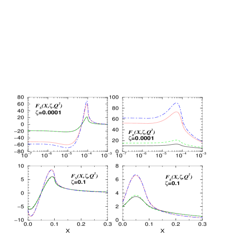
FIG. 3.: Unpolarized NLO input and evolved singlet quark and gluon GPDs at small and large skewedness. The solid curves are the input MRSA${}^{{}^{\prime}}$ GPDs at $Q_{0}=2~{}\mbox{GeV}$, the dotted ones show them evolved to $Q=10~{}\mbox{GeV}$. The dashed curves are input GRV98 GPDs at $Q_{0}=2~{}\mbox{GeV}$ and the dashed-dotted ones show them evolved to $Q=10~{}\mbox{GeV}$. The quark singlet is scaled by a factor of $10^{-4}$ at $\zeta=0.0001$ and by $10^{-2}$ at $\zeta=0.1$. For $\zeta=0.1$ the symmetry of the gluon GPD and the anti-symmetry of the singlet quark GPD are apparent about the point $X=\zeta/2=0.05$.

In the upper plot of fig.(2) we show the same ratio for the unpolarized evolved gluon distribution of GRV98 [36]. It is interesting and somewhat surprising to observe that this ratio drops progressively below unity even for $X\gg\zeta$ as $Q^{2}$ increases, and is as much as $6\%$ below at $X=0.001$ for $Q=10$ GeV. However, on inspecting the ratio of the NLO $gg$ and $gq$ kernels for the GPDs to the NLO $gg$ and $gq$ kernels of the forward PDFs, one observes that even for $X\gg\zeta$ they can be very different from one another over a broad range of $X$, but will eventually settle at unity. An enhancement due to skewed evolution is still seen at NLO , but only very close to $X=\zeta$ (for both the polarized and unpolarized cases).

In the lower plot of fig.(2) we illustrate the polarized case using the GS(A) polarized gluon. Again we see the ratio drop progressively below unity for $X>\zeta$. The size of the effect is similar, although this is difficult to see directly since the ratio of GPD to PDF is already smaller than unity at the input scale (for $X\approx\zeta$) [37].

B NLO GPDs and a comparison with LO

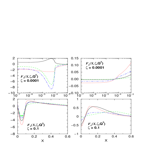
FIG. 4.: Polarized NLO input and evolved singlet quark and gluon GPDs at small and large skewedness. The solid curves are the input GS(A) GPDs at $Q_{0}=2~{}\mbox{GeV}$, the dotted ones show them evolved to $Q=10~{}\mbox{GeV}$. The dashed curves are input GRSV00 GPDs at $Q_{0}=2~{}\mbox{GeV}$ and the dashed-dotted ones show them evolved to $Q=10~{}\mbox{GeV}$. The quark singlet is scaled by a factor of $10^{-2}$ at $\zeta=0.0001$. For $\zeta=0.1$ the symmetry of the polarized singlet quark GPD and the anti-symmetry of the polarized gluon GPD are apparent about the point $X=\zeta/2=0.05$.

In figs.(3,4, 5) we present the input and evolved unpolarized and polarized GPDs, respectively, for the singlet quark and gluon, and are encouraged to note that they are smooth, continuous functions of $X$. The lower plots in figs.(3,4), with $\zeta=0.1$, use a linear scale on the $X$ axis, and hence illustrate very explicitly the symmetries in the ERBL region about the point $X=\zeta/2=0.05$ which are manifestly preserved under evolution. These symmetries also hold for the upper curves (for $\zeta=0.0001$) but are less visible on a logarithmic scale. These features indicate that our code is indeed correct and properly performs the NLO evolution in both the ERBL and DGLAP region. From fig.(3) and the upper plots of fig.(5) we note that both unpolarised input sets (GRV98 and MRSA’) produce similar results for the input and evolved GPDs.

From fig.(4) and the lower left plot of fig.(5) we note with particular interest the result for the NLO evolution of the polarized quark singlet at small $\zeta$. The GS(A) set assumes a rather different sea content to GRSV00, in particular the former has a positive quark singlet at the input scale and the latter a negative one. The NLO evolution keeps the GRSV00 distribution unchanged in shape, only altering its size, whereas the GS(A) distribution is driven towards the same shape as well as overall sign as the GRSV00 distribution. This seems to indicate that the NLO generalised evolution favours the initial shape of the GRSV00 distribution and thus a negative polarized quark singlet at small $\zeta$. At larger $\zeta$, where the sea is of little numerical importance, the initial shapes are very similar and so one does not observe the same type of effect for GS(A).

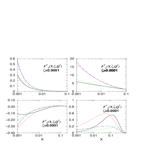
FIG. 5.: Polarised (“A”) and unpolarised (“V”) singlet quark and gluon GPDs for $\zeta=0.0001$ in the $X>10\zeta$ region. The input parton sets for each curve are the same as those given in Figs. 3 and 4. The quark singlet is scaled by a factor of $10^{-4}$ in the unpolarised case and by $10^{-2}$ in the polarised case.

Although similar in shape (except for the polarized quark singlet at the input), the two sets of polarised distributions differ considerably in size. The general evolution effects which push partons to smaller $X$ with increasing $Q^{2}$, are naturally the same for both sets of inputs.

In order to quantify the relative effects of including NLO skewed kernels in detail, we also evolved the same input GPDs using LO skewed kernels. In the upper and lower plots of fig.(6) we present the ratio of the evolved GPDs at NLO to those at LO, for the unpolarized and polarized cases, respectively. Overall the effect of including NLO corrections is at most a $25\%$ effect, within the kinematic ranges illustrated. The regions furthest from unity in these ratio plots illustrate the ranges in $X$, relative to $\zeta$, where the greatest effects are felt. The symmetry of the individual distributions about $\zeta/2$ continue to be reflected in these ratio plots, which further indicates that the NLO evolution slightly alters the shape of the distributions relative to LO, but in such a way as to preserve the symmetries.

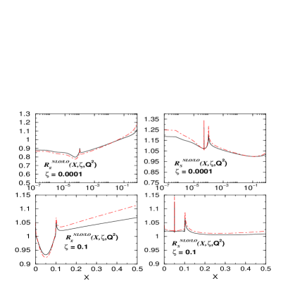
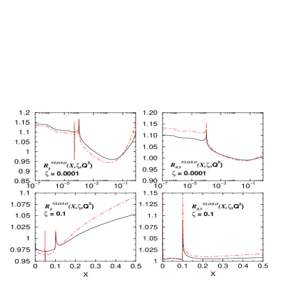
FIG. 6.: The ratio of NLO to LO evolved GPDs for the unpolarized (upper plot, MRSA${}^{{}^{\prime}}$) and polarized (lower plot, GRSV) cases. The solid and dashed-dotted curves shows the ratio at $Q=5~{}\mbox{GeV}$ and $Q=10~{}\mbox{GeV}$ , respectively.

The spikes in the antisymmetric unpolarized singlet quark and polarized gluon ratios result from a slight loss of numerical accuracy in a few bins around the point $\zeta/2$ (where the distributions have to pass through zero). The effect is magnified in this ratio. However, since the distributions vary by as much as twelve orders of magnitude (in the unpolarized quark singlet case), and the effect occurs close to a zero, this is not a cause for concern.

The cusps observed at $X=\zeta$ are due to the fact that the NLO over LO ratios approach the same value from the ERBL and DGLAP region very rapidly around the $X=\zeta$ region. This change in shape in NLO over LO, which could be seen more clearly if the region around the $X=\zeta$ were to be enlarged, is easily explained. In the LO kernels, rational functions of the type $1/(X-\zeta)$ appear, which however combine to form a function which is finite at the point $X=\zeta$. In NLO, functions of the type $\ln^{n}(X-\zeta)/(X-\zeta)^{n_{1}}$ with $n,n_{1}=0,1,2$ appear, where again the rational functions cancel, but the logarithms do not. This leads to an integrable logarithmic singularity at NLO of a similar type as encountered in the NLO forward evolution, at the lower bound of the convolution integral in the RGE, $y=x_{bj}$, and leads to a strong enhancement of the NLO distributions in the region around $X=\zeta$ as seen in the figures. The ratio of NLO to LO in the unpolarized case for GRV98 are very similar, within a few percent, to the plotted MRSA${}^{{}^{\prime}}$. In the polarized case the contrast is larger, until very large $Q^{2}$, due to the markedly different input functions used for GRSV and GS(A)[38].

C Influence of the D-term

FIG. 7.: The influence of including the D-term on the GRV98-model quark singlet GPD at the input scale in the ERBL region $X<\zeta$, for various values of $\zeta$. The anti-symmetry which the D-term shares with the singlet, about $X=\zeta/2$, is manifest by the symmetry about $X=\zeta/2$ in this ratio plot.

Recall that in the definition of the unpolarized singlet-type quark input GPDs we included an extra piece in the ERBL region only, known as the D-term, which we modelled following [25] in eq.(59). This extra piece simply forms part of the definition of the input which is then evolved. In order to quantify its influence we consider in fig.(7) the ratio of the quark singlet with the D-term included to that with it omitted for various values of $\zeta$. One observes that its numerical influence becomes progressively less significant as $\zeta$ decreases (at $\zeta=0.01$ it is less than $1\%$).

D Influence of the profile functions

In section III we specified in eq.(40) specific cases of Radyushkin model [12, 13] for GPDs based on double distributions. The original model specified a more general form for the profile functions:

$$\pi(x,y)=\frac{\Gamma(2b+2)}{2^{2b+1}\Gamma^{2}(b+1)}\frac{[(1-|x|)^{2}-y^{2}]^{b}}{(1-|x|)^{2b+1}}\,.$$ (83)

So that eq.(40) corresponds to $b=1$ for the quark and $b=2$ for the gluon. It was suggested in [25] that variable $b$ could be used as a fit parameter to extract GPDs from DVCS observables. It was also noted that the limit of very large $b$ corresponds to the forward limit of $\zeta$-independent GPDs, for all $X>\zeta$.

We have investigated this issue numerically and find that in the DGLAP region the GPDs tend to the PDFs very slowly as a function of $b$, particularly close to $X=\zeta$. Meanwhile the behaviour of the GPDs in the ERBL region is seen to change dramatically. We illustrate this in fig. 8 at small and large $\zeta$ (i.e. $\zeta=0.0001,0.1$, respectively), comparing $b=100$ with the canonical values for both the quark singlet and gluon, using GRV98 forward distributions. As can be seen, in the DGLAP region ($X>\zeta$) using such a large value of $b$ has only a marginal effect. In the ERBL region a rather dramatic effect is seen at the input scale, particularly close to the symmetric point $X=\zeta/2$. It is satisfying to observe (from the $Q=10$ GeV curves) that under evolution both choices appear to tend to similar evolved distributions (as the memory of the details of the input distribution are washed out by the skewed evolution). We may conclude from the figures that if parameter $b$ is to be used as a fit parameter to constrain GPDs using data, it would require high statistics data on DVCS observables which are very sensitive to the details of the real part of DVCS amplitudes in the ERBL region, such as the azimuthal angle asymmetry or the charge asymmetry (see e.g. [29]). We may also conclude that taking the very large $b$ limit of Radyushkin’s ansatz is not a particularly good way of numerically probing models in which the GPD is the same as the PDF in the DGLAP region, since the convergence appears to be very slow.

FIG. 8.: Sensitivity of the input ($Q=2$ GeV) and evolved ($Q=10$ GeV) GPDs to the choice of the parameter $b$ for the profile functions in eq.(83). We compare large $b=100$ with the canonical values of eq.(40) ($b=1.0$ for the quark singlet and $b=2$ for the gluon), using GRV98 forward distributions at both small $\zeta=0.0001$ and large $\zeta=0.1$ skewedness (right and left hand plots respectively). The $b=100$ case is shown with thickened lines.

VI Conclusions

In this paper we have presented a complete numerical solution for the next-to-leading order (NLO) evolution equations for polarized and unpolarized generalised parton distributions (GPDs). We demonstrated that our solutions stay smooth and preserve all the symmetries of GPDs, giving us confidence in the correctness of our numerical implementation. We presented the relative effect of moving from leading-order (LO) to NLO for a common input. We illustrate the effect of NLO skewed evolution on the magnitude and shape of two correctly-symmetrized input models based on conventional parton density functions, for two values of the skewedness parameter, $\zeta=0.0001,0.1$, typical of HERA and HERMES kinematics. We demonstrate that in NLO, in contrast to LO, for small skewedness, the ratio of GPD gluon to PDF gluon in the unpolarized case does not have to be larger than unity in the $\overline{MS}$ scheme employed here. This new effect is directly relevant to the study of small-$x$ exclusive diffractive vector meson and real photon production at HERA. The next step is to use these NLO GPDs to make NLO predictions for measurable physical processes [39, 40, 41], such as DVCS, at HERA [7, 8], HERMES [9] and Jefferson Lab [10]. A detailed and direct comparison with all available data from a wide range of experimental observables is ultimately required to establish accurately the details of the GPDs.

REFERENCES

- [1] D. Müller et al., Fortschr. Phys. 42 (1994) 101.
- [2] X. Ji, Phys. Rev. D55 (1997) 7114.
- [3] A. V. Radyushkin, Phys. Rev. D56 (1997) 5524.
- [4] J. C. Collins, L. Frankfurt, M. Strikman, Phys. Rev. D 56 (1997) 2982.
- [5] J. C. Collins, A. Freund, Phys. Rev. D59 (1999) 074009.
- [6] X. Ji, J. Osborne, Phys. Rev. D58 (1998) 094018.
-
[7]
P.R. Saull, for ZEUS Collab., “Prompt photon production and observation of deeply virtual Compton scattering”,
Proc. EPS 1999, July 1999, Tampere, Finland, hep-ex/0003030;
ZEUS Collab., “Measurement of the deeply virtual Compton scattering cross section at HERA”, Abstract 564, IECHEP 2001, July 2001, Budapest, Hungary. -
[8]
C. Adloff et al., H1 Collab., Phys. Lett. B517 (2001) 47;
L. Favart, for H1 Collab., “Deeply virtual Compton scattering at HERA”, Proc. ICHEP 2000, July 2000, Osaka, Japan, hep-ex/0101046. - [9] A. Airapetian et al., Hermes Collab., Phys. Rev. Lett. 87 (2001) 182001.
-
[10]
S. Stepanyan et al., CLAS Collab., Phys. Rev. Lett. 87 (2001) 182002;
J. P. Chen, for Jefferson Lab,
http://www.jlab.org/~sabatie/dvcs/index.html; - [11] A. V. Belitsky, A. Freund and D. Müller, Nucl. Phys. B574 (2000) 347.
- [12] A. V. Radyushkin, Phys. Rev. D59 (1999) 014030.
- [13] A. V. Radyushkin, Phys. Lett. B449 (1999) 81; I. V. Musatov and A. V. Radyushkin, Phys. Rev. D61 (2000) 074027.
- [14] A. D. Martin, R. G. Roberts and W. J. Stirling, Phys. Lett. B354 (1995) 155.
- [15] T. Gehrmann and W. J. Stirling, Phys. Rev. D53 (1996) 6100.
- [16] M. Glück, E. Reya and A. Vogt, Eur. Phys. J. C5 (1998) 461.
- [17] M. Glück et al., Phys. Rev. D63 (2001) 094005
- [18] A solution to the RGEs at NLO has been presented at large in [19, 20], however due to technical problems the methods used could not be applied at smaller .
- [19] A. V. Belitsky et al., Phys. Lett. B 437 (1998) 160.
- [20] A. V. Belitsky et al., Phys. Lett. B474 (2000) 163.
- [21] V. Guzey and A. Freund, Phys. Lett. B462 (1999) 178; “Numerical methods in the LO evolution of non-diagonal parton distributions: the DGLAP case”, hep-ph/9801388.
- [22] K. J. Golec-Biernat and A. D. Martin, Phys. Rev. D59 (1999) 014029.
- [23] http://durpdg.dur.ac.uk/hepdata/dvcs.html
- [24] M. V. Polyakov and C. Weiss, Phys. Rev. D60 (1999) 114017.
- [25] N. Kivel, M. V. Polyakov and M. Vanderhaeghen, Phys. Rev. D 63 (2001) 114014.
- [26] M. Penttinen, M. V. Polyakov and K. Goeke, Phys. Rev. D 62 (2000) 014024.
- [27] V. N. Gribov and L. N. Lipatov, Sov. J. Phys 15 (1972) 438, 675; Yu. L. Dokshitzer, Sov. Phys. JETP 46 (1977) 641; G. Altarelli. and G. Parisi, Nucl Phys B126 (1977) 298.
- [28] A. V. Efremov and A. V. Radyushskin, Theor. math. Phys. 42 (1980) 97, Phys Lett. B94 (1980) 245; G. P. Lepage and S. J. Brodsky, Phys Lett. B87 (1979) 359; Phys. Rev. D22 (1980) 2157.
- [29] A. V. Belitsky et al., Nucl. Phys. B593 (2001) 289.
- [30] The starting scale for GRV98 and GRSV00 are rather low. In order to make a meaningful comparison of the effects of skewedness, we evolve both polarized and unpolarized distributions to the common input scale of GeV before introducing skewedness into the evolution. For computational reasons, we also found it convenient to use a faithful multi-parameter fit to these GRV and GRSV distribution rather than using the codes provided by the authors. For GRSV00 we choose the “standard scenario” option of unbroken polarised sea distributions.
- [31] The endpoint () concentrated terms in eqs.(63,76) can be found in [11] and are determined by the requirement that the zeroth order conformal moment of the kernel has to be zero. Note that in the numerical implementation of the evolution the pure singlet component in the kernel in both DGLAP and ERBL regions is not regularized (for more details see [11]).
- [32] http://www.phys.psu.edu/~cteq/#PDFs
- [33] L. Frankfurt, M. McDermott and M. Strikman, JHEP 9902 (1999) 002.
- [34] B. Pire, J. Soffer and O. V. Teryaev, Eur. Phys. J. C8 (1999) 103.
- [35] It was not applicable, even at LO, in the polarized case.
- [36] A slight deviation of the ratio from unity is observed in the plot for because for GRV98, we use an analytic fit to the actual distributions at our input scale. This fit starts to deviate slightly from the results produced by the FORTRAN routines of GRV98 at the input scale. The NLO evolution enhances this difference and thus we do not expect the ratio to approach unity precisely for large . Note however that the deviation is at most . The small wiggles in the curves are artifacts of the fitting procedure since we normalise to the code of GRV98.
- [37] Small deviations from unity are observed at very large for evolved scales. This results from the fact that in our input GPDs we directly implement eqs.(9,10,13) and tables.(1,2) of [15] (gluon A) analytically and the resultant numbers deviate slightly from those obtained from the grid-based FORTRAN routine provided by Gehrman-Stirling at such large . Since we use the latter to normalise this ratio we do not expect to reproduce the forward limit with perfect accuracy.
- [38] In the quark case, we used only the singlet type combination of the down quark since it does not change sign as the up and the strange do. A change in sign distorts ratio plots by a large ratio around the point where the distributions changes sign, since this particular point is shifted towards lower in NLO compared to LO.
- [39] A. Freund and M. McDermott, Phys. Rev. D65 (2002) 091901(R).
- [40] A. Freund and M. McDermott, Phys. Rev. D65 (2002) 074008.
- [41] A. Freund and M. McDermott, Eur. Phys. J. C23 (2002) 651.