Abstract

The ideal neutrino detector at the neutrino factory should have a mass in the range of 10 kton, provide particle identification to tag the flavor of the incoming neutrino, lepton charge measurement to select the incoming neutrino helicity, good energy resolution to reconstruct the incoming neutrino energy, and be isotropic to equally well reconstruct incoming neutrinos from different baselines (it might be more efficient to build various sources at different baselines, than various detectors). The detector should also be able to reconstruct neutrino event typically below 15 GeV. A detector with such quality is most adapted to fully study neutrino oscillations at the neutrino factory. In particular, measurement of the leading muons and electrons charge is the only way to fully simultaneously explore $CP$ and $T$ violation effects. We think that a magnetized liquid argon imaging detector stands today as the best choice of technique, that holds the highest promises to match the above mentioned detector requirements. We discuss also the optimal neutrino factory energy and baseline between source and detector in order to best perform these studies.

1 Introduction

The first generation long baseline (LBL) experiments — K2K [1], MINOS [2], OPERA [3] and ICARUS [4, 5] — will use artificial neutrino beams produced by the “traditional” meson-decay method, to search for a conclusive and unambiguous signature of the neutrino flavor oscillation [6] observed in cosmic ray neutrinos [7]. These experiments will provide the first precise measurements of the parameters governing the main muon disappearance mechanism.

In contrast, a neutrino factory[8, 9] is understood as a machine where low energy muons of a given charge are accelerated to high energy, and let decay into one electron and two neutrinos within a muon storage ring.

The great physics potential of a neutrino factory comes from its ability to test in a very clean and high statistics environment all possible flavor oscillation transitions [10, 11]. This ability will provide very stringent information on all the elements of the neutrino mixing matrix and on the mass pattern of the neutrinos.

In a $3\times 3$-mixing scenario, the mixing matrix, which should be unitary, is determined by three angles and a complex phase. Neutrino factories will provide precise determinations of two angles and of the largest mass difference[10, 11]. In addition, a test of the unitarity of the matrix could be performed[11].

Apart from being able to measure very precisely all the magnitude of the elements of the mixing matrix, the more challenging and most interesting goal of the neutrino factory is the search for effects related to the complex phase of the mixing matrix[12]. The complex phase will in general alter the neutrino flavor oscillation probabilities, and will most strikingly introduce a difference of transition probabilities between neutrinos and antineutrinos (CP-violation effects), and between time-reversed transitions (T-violation effects). Neutrino factories should provide the intense and well controlled beams needed to perform these studies.

It should be stressed that the complete and comprehensive detection of $T$- and/or $CP-$violation effects is very difficult for terrestrial experiments, as it requires $L/E_{\nu}$ values simultaneously in the range of solar and atmospheric neutrinos. In addition, they require that the transitions ${\nu_{e}}\rightarrow{\nu_{\mu}}$, $\bar{\nu_{e}}\rightarrow\bar{\nu_{\mu}}$, ${\nu_{\mu}}\rightarrow{\nu_{e}}$ and $\bar{\nu_{\mu}}\rightarrow\bar{\nu_{e}}$ be measured, a priori within the same experiment. It has been known[10] that only in the case of the LMA solution to the solar neutrino problem, can one hope to look for effects related to the complex nature of the mixing matrix. We assume that this is the case.

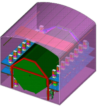
Figure 1: View of the planned MINOS detector. The detector with a total mass of 5.4 kton should start data taking with the FNAL-NUMI beam in 2004.

2 Detectors at the neutrino factory

We briefly mention the kind of detectors that are currently envisaged in the context of the neutrino factory.

2.1 Magnetized steel-scintillator sandwich

This is the “traditional” neutrino detector, with a lot of experience gained with (though smaller) detectors like CCFR/NuTeV or CDHS. A detector based on iron has the advantage of having a high density and to be easily magnetizable, for a “straight-forward” $\mu^{+}/\mu^{-}$ discrimination. It has sufficient granularity to only cleanly detect muons, and offers a rather poor discrimination and reconstruction of electrons and neutral-current-like events (including hadronic decays of taus). The muon resolution is good and the jet energy resolution is reasonable (typ. $80\%/\sqrt{E_{h}}$). A minimum muon energy threshold (typ. 4-6 GeV) is needed in order to separate the muon from other hadrons and the muon separation from the jet is difficult to measure. The electron/hadron discrimination is rather poor. The angular resolution is determined by the transverse readout segmentation, which is in fact rather modest. The full volume of the detector has to be instrumented, and by nature of the sandwich, the readout is not very isotropic. Hence, a detector optimized to reconstruct “horizontal” events from an artificial neutrino beam coming from a well defined direction, will not at the same time provide good reconstruction of say atmospheric events coming from “above” and “below”. One considers as prototype for the neutrino factory the MINOS[2] detector (see Figure 1), that should reach a mass of 5.4 kton in 2003. It is composed of 486 layers of 2.45cm Fe each, divided into two sections each 15 m long. The field has an average value of 1.3 T. Since detector construction is under way, we shall soon learn if this detector technology can be scaled to the larger masses currently envisaged for a neutrino factory, namely in the range of 40 kton.

2.2 Large water-Cerenkov

This is a well-proven technology (IMB, Kamiokande, SuperKamiokande). The target material (Water) is cheap and only the surface of the detector (and not the volume unlike in the previous magnetized steel-scintillator sandwich) needs to be instrumented, hence this technology scales well to gigantic masses. The size will eventually be limited by water properties. A next generation 500 kton is under consideration[14]. The reconstruction of events is rather isotropic, and this kind of detector will certainly cover a broad physics program, including observation of atmospheric neutrinos, maybe solar neutrinos if energy threshold allows it, supernova neutrinos, and search for proton decays. The clear disadvantage of this kind of detector is that the reconstructed pattern is limited to “simple event topologies”, that are not really compatible with a detailed reconstruction of neutrino events with complicated final states. See Figure 2. The detection of the muon charge cannot be easily implemented in water and should rely on a downstream muon identifier.

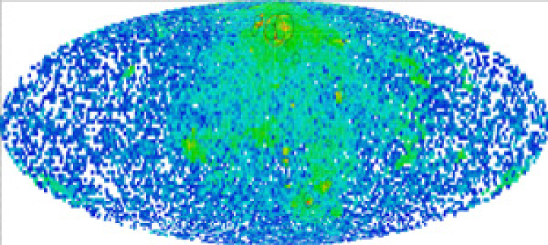
Figure 2: Simulated neutrino event from a 50 GeV storage ring.

2.3 Emulsion/target sandwich

The ECC (Emulsion Cloud Chamber) technique currently envisaged for OPERA [3] has been used successfully in the DONUT[13] experiment, though in a very small scale compared to what is needed for a neutrino factory. The technique should be demonstrated at the 1 kton scale at the LNGS by the year 2005. Emulsions have a fantastic granularity (at the level of microns) and can be used to directly detect the kink in the decay of a charged tau lepton. In OPERA, emulsions will be used as very precise tracking devices to reconstruct pieces of tracks, whereas actual neutrino interactions will occur in a passive target material (Pb). The non-alignment of the track segments reconstructed over a thickness of about 100 microns of two consecutive emulsion layers, will indicate potential decay kinks. A direct search for ${\nu_{e}}\rightarrow{\nu_{\tau}}$ at a neutrino factory could be attempted if the charge of the tau can be detected to suppress the ${\nu_{\mu}}\rightarrow{\nu_{\tau}}$ “background”. The most obvious disadvantages are the difficulty to scale this detector to very large masses, the potentially very large amount of scanning involved in a high-statistics experiment at a neutrino factory and possibly a severe background from charm decays produced in ${\nu_{e}}$ interactions.

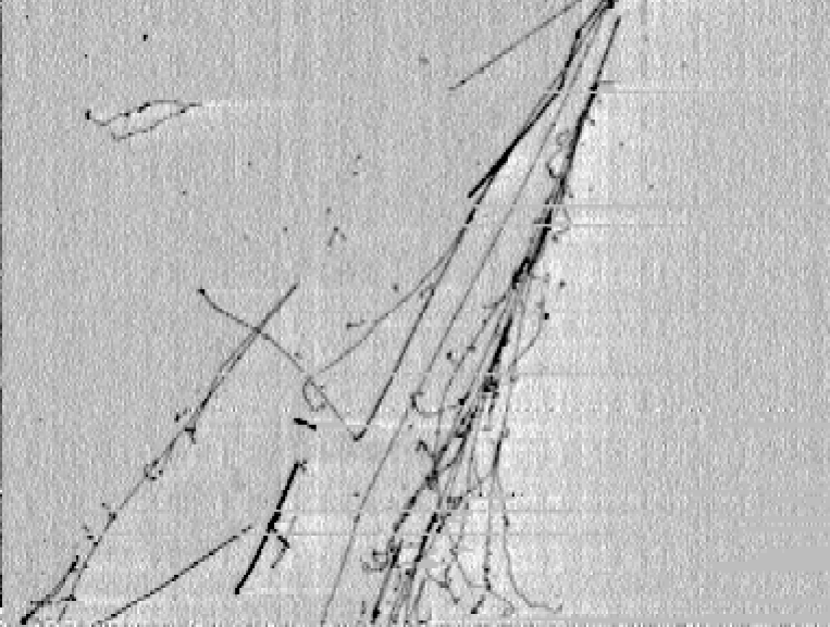
Figure 3: Electronic liquid argon imaging of a cosmic ray induced shower. The overall drift time (horizontal axis) corresponds to about 40 cm of drift distance. The vertical co-ordinate is the wire numbering; around 40 cm are shown.

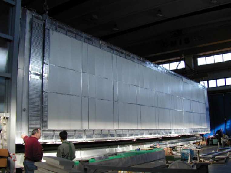
Figure 4: Side view during installation of one of the two cryostats that compose the ICARUS T600 detector.

2.4 Liquid Argon imaging TPC

The liquid argon imaging technique provides fully bubble-chamber-like reconstruction of events (See Figure 3). It is fully a homogeneous, continuous, precise tracking device with high resolution $dE/dx$ measurement and full sampling electromagnetic and hadronic calorimetry. Imaging provides excellent electron identification and electron/hadron separation. Energy resolution is excellent (typ. $3\%/\sqrt{E}$ for e.m. showers) and the hadronic energy resolution of contained events is also excellent (typ. $30\%/\sqrt{E_{h}}$).

Like with the water Cerenkov detector, liquid argon detectors cover a broad physics program, including observation of atmospheric neutrinos, solar neutrinos, supernova neutrinos, and search for proton decays.

One disadvantage in the current implementation is the lack of magnetic field. One has in principle to rely on a down-stream muon spectrometer (that has however low threshold given the loss in Argon of $240~{}MeV/m$). Magnetization was considered in the past[15], and a possibility to magnetize the large, multikton, volume of Argon is however under study[16]. This method is the only one, most easily scalable to multikton mass range, that would provide sufficient granularity to measure the charge of electrons (see Section 5).

Liquid argon imaging, though a priori more difficult to implement than say a magnetized iron-scintillator sandwich, is becoming a mature technique, that has so far been demonstrated up to the 15 ton prototype scale. The next major milestone is the operation of the ICARUS 600 ton prototype (see Figure 4). Its construction has been completed during 2000, in all its various components. The first technical run has started in March 2001. Cosmic muon tracks have been seen in June 2001. The successful reaching of this milestone is very important, and after a series of other technical tests to be performed in the assembly hall within the summer 2001, the detector should be ready to be transported to the LNGS tunnel by middle 2002. The physics program achievable with the T600 detector has been described in Ref.[5]. It covers the observation and study of atmospheric and solar neutrinos.

3 The oscillation physics at the neutrino factory

Neutrino sources from muon decays provide clear advantages over neutrino beams from pion decays. The exact neutrino helicity composition is a fundamental tool to study neutrino oscillations. It can be easily selected, since $\mu^{+}\rightarrow e^{+}{\nu_{e}}\bar{\nu_{\mu}}$ and $\mu^{-}\rightarrow e^{-}\bar{\nu_{e}}{\nu_{\mu}}$ can be separately obtained.

At a neutrino factory, one could independently study the following flavor transitions:

$$\mu^{-}\rightarrow e^{-} \bar{\nu_{e}} {\nu_{\mu}}$$ (3)

$$\rightarrow{\nu_{e}}\rightarrow e^{-}\rm\ appearance$$

$$\rightarrow{\nu_{\mu}}\rm\ disappearance,\ same\ sign\ muons$$

$$\rightarrow{\nu_{\tau}}\rightarrow\tau^{-}\rm\ appearance,\ high\ energy\ nu^{\prime}s$$

$$\rightarrow \bar{\nu_{e}}\rm\ disappearance$$ (4)

$$\rightarrow \bar{\nu_{\mu}}\rightarrow\mu^{+}\rm\ appearance,\ wrong\ sign\ muons$$ (5)

$$\rightarrow \bar{\nu_{\tau}}\rightarrow\tau^{+}\rm\ appearance,\ high\ energy\ nu^{\prime}s$$ (6)

plus 6 other charge conjugate processes initiated from $\mu^{+}$ decays.

The ideal neutrino detector should be able to measure these 12 different processes as a function of the baseline $L$ and of the neutrino energy $E_{\nu}$!

Of particular interest are the charged current neutrino interactions, since they can in principle be used to tag the neutrino flavor and helicity, through the detection and identification of the final state charged lepton:

$$\nu_{\ell}N\rightarrow\ell^{-}+hadrons\ \ \ \ \ \bar{\nu}_{\ell}N\rightarrow\ell^{+}+hadrons$$ (7)

We illustrate this in the case of a non-magnetized ICARUS-like detector. Figures 8, 8, 8 and 8 show the reconstructed visible energy at the baseline $L=7400$km normalized to $10^{20}\mu$’s for each event class for a specific oscillation scenario with $\Delta m_{32}^{2}=3.5\times 10^{-3}$ eV², $\sin^{2}\theta_{23}=0.5$ and $\sin^{2}2\theta_{13}=0.05$. The different contributions including backgrounds for each event class have been evidenced in the plots. For example, in Figure 8, the different processes that contribute to the right-sign muon class are unoscillated muons, taus and background events.

Hence, the ideal detector at the neutrino factory should possess the following characteristics:

• Particle identification: the detector should be able to identify and measure the leading charged lepton of the interaction, in order to tag the incoming neutrino flavor.

• Charge identification: the sign of the leading lepton charge should be measured, since it tags the helicity of the incoming neutrino.

• Energy resolution: the incoming neutrino energy $E_{\nu}$ is reconstructed as $E_{\nu}=E_{\ell}+E_{had}$, where $E_{\ell}$ is the leading lepton energy and $E_{had}$ is the hadronic energy. Hence, detector with better energy resolution will reconstruct the parameter of the incoming neutrino better, and therefore the oscillation probability.

• Low energy threshold: the reconstruction and identification should be fully efficient for neutrino events below 15 GeV, as it is in this region that we expect the cleanest and most ambiguous signal from $CP$ and $T$ violation, as we will demonstrate in the Sections 9 to 12.

• Isotropic: one might want to perform various similar experiments at different baselines. The probably most efficient way to achieve this is to build a large neutrino detector, isotropic in nature, capable of measuring equally well neutrinos from different sources located at different baselines $L$. Because of the spherical shape of the Earth, sources located at different baselines $L$ will reach the detector “from below” at different angles.

It should be stressed that these features need to be implemented on detectors which have to be very massive. Indeed, the neutrino factory will clearly be more intense (by at least one order of magnitude) than current neutrino beams. However, the requirement to make precision measurements and the considered rather long baselines (neutrino flux scales as $L^{-2}$), implies that detector in the range of 10 kt or more will be required.

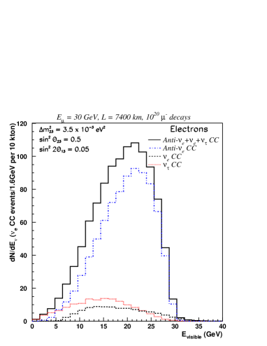
Figure 5: Visible energy spectrum for electron events: $\nu_{e}$ CC (dashed line), $\nu_{\tau}$ and $\bar{\nu}_{\tau}$ (dotted line) and $\bar{\nu}_{e}$ CC (dot-dashed). The solid histogram shows the sum of all contributions.

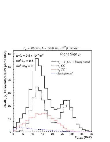
Figure 6: same as Figure 8 for right-sign muon sample: $\nu_{\mu}$ CC (dashed line), $\nu_{\tau}$ and $\bar{\nu}_{\tau}$ (dotted line) and meson decay background (dot-dashed). The solid histogram shows the sum of all contributions.

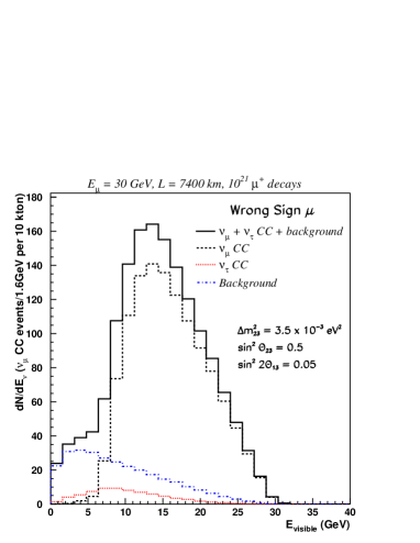
Figure 7: same as Figure 8 for wrong sign muon sample: $\nu_{\mu}$ CC (dashed line), $\nu_{\tau}$ and $\bar{\nu}_{\tau}$ (dotted line) and meson decay background (dot-dashed). The solid histogram shows the sum of all contributions.

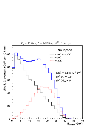
Figure 8: same as Figure 8 for the no-lepton sample: $\nu$ NC (dashed line), $\nu_{\tau}$ and $\bar{\nu}_{\tau}$ (dotted line). The solid histogram shows the sum of all contributions.

4 Detection of muons, electrons, taus and neutral currents

Clearly, the goal to identify and measure all possible final state leptons produced in charged current neutrino interactions as well as neutral current neutrino interactions imposes some constraints on the detector technology.

The most stringent problem is related to the achievable granularity in a given detector configuration. Indeed, the requirement that detectors should have a fiducial mass beyond the kton range immediately brings in various choices and optimizations, since in first approximation, the total cost of the detector will depend on its mass times its granularity. It is therefore possible to opt for a poor granularity detector of very large mass, or a high granularity detector of a smaller mass. In between these two extremes one can have a continuous set of possible optimizations.

When we consider the possibility to tag the outgoing lepton, we can subdivide the requirements as a function of the lepton type:

• Muons: the detection of muons is straight-forward. In principle, one looks for penetrating particles. In practice, one has however to be careful of backgrounds (misidentification) coming from $\pi^{\pm}$, $K^{\pm}$ decays and from charm semileptonic decays.

• Electrons: the detection of electrons is harder. In principle, one looks for large and “short” energy deposition. In practice, one needs to carefully separate electrons from $\pi^{0}$ conversions. Different levels of expertise have been developed in the field, yielding typically background rejections ranging from 1-2% (for the worst granularity) to better than $10^{-3}$ for the best granularity.

• Taus: the detection of tau leptons is the hardest. One can attempt to look on an-event-by-event basis for the tau “kink”; this however requires an extremely good reconstruction of the neutrino vertex. The required resolution has so far only been achieved with the help of photographic emulsions, which pose stringent constraints in scanning, and are strongly cost limited. Another possibility is to provide a “statistical separation”. In particular, 60% of the tau decays are into 1-prong, 3-prong or more hadrons and hence look like neutral current events (i.e. without final state leading electron or muon).

As far as the detection of the lepton charge is concerned, here also the level of difficulty depends strongly on the type of lepton. In general, one has to rely on a magnetic analysis to measure the charge.

• Muons: the measurement of the muon charge is relatively easy, since tracks produced by muons are long. One can either envisage a fully magnetized target or rely on a down-stream spectrometer.

• Electrons: the measurement of the electron charge is the hardest. One needs to measure significantly precisely the bending in the magnetic field before the start of the electromagnetic shower. Hence, the measurement is typically limited to a few $X_{0}$.

• Taus: when the tau decays into a muon, then the measurement is easy. Otherwise, one needs to rely on a very high granularity and magnetized target, in order to identify the tau, its decay products and eventually reconstruct the mother charge from the charge of the decay products.

5 Measurement of the electron charge in liquid argon

We saw that liquid argon imaging provides very good tracking with $dE/dx$ measurement, and excellent calorimetric performance for contained showers. This allows for a very precise determination of the energy of the particles in an event. This is particularly true for electron showers, which energy is very precisely measured.

The possibility to complement these features with those provided by a magnetic field has been considered. Embedding the volume of argon into a magnetic field would not alter the imaging properties of the detector and the measurement of the bending of charged hadrons or penetrating muons would allow a precise determination of the momentum and a determination of their charge.

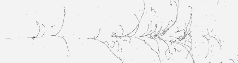
Figure 9: Magnetized liquid argon TPC: simulation of the 2.5 GeV electron shower in liquid argon. The field has a strength B=1.5 T and is directed perpendicular to the sheet-plane.

We have recently started studying the effect of the magnetic field on electrons (see Figure 9). Unlike muons or hadrons, the early showering of electrons makes their charge identification difficult. We however found that the determination of the charge of electrons of energy in the range between 1 and 5 GeV is feasible with good purity, provided the field has a strength in the range of 1 Tesla. Preliminary estimates show that these electrons exhibit an average curvature sufficient to have electron charge discrimination better than $1\%$ with an efficiency of 20%.

6 CP and T violation measurements

In a three-family neutrino oscillation scenario, the flavor eigenstates $\nu_{\alpha}(\alpha=e,\mu,\tau)$ are related to the mass eigenstates $\nu^{\prime}_{i}(i=1,2,3)$ by the mixing matrix U

$$\nu_{\alpha}=U_{\alpha i}\nu^{\prime}_{i}$$ (8)

and it is customary to parameterize it as:

$$U(\theta_{12},\theta_{13},\theta_{23},\delta)=\left(\begin{tabular}[]{ccc}$c_{12}c_{13}$&$s_{12}c_{13}$&$s_{13}e^{-i\delta}$\\ $-s_{12}c_{23}-c_{12}s_{13}s_{23}e^{i\delta}$&$c_{12}c_{23}-s_{12}s_{13}s_{23}e^{i\delta}$&$c_{13}s_{23}$\\ $s_{12}s_{23}-c_{12}s_{13}c_{23}e^{i\delta}$&$-c_{12}s_{23}-s_{12}s_{13}c_{23}e^{i\delta}$&$c_{13}c_{23}$\end{tabular}\right)$$ (9)

with $s_{ij}=\sin\theta_{ij}$ and $c_{ij}=\cos\theta_{ij}$.

We concentrate on transitions between electron and muon neutrinos. The oscillation probability is

$$P(\nu_{e}\rightarrow\nu_{\mu})=P(\bar{\nu}_{\mu}\rightarrow\bar{\nu}_{e})=$$

$$4c^{2}_{13}\Bigl{[}\sin^{2}\Delta_{23}s^{2}_{12}s^{2}_{13}s^{2}_{23}+c^{2}_{12}\left(\sin^{2}\Delta_{13}s^{2}_{13}s^{2}_{23}+\sin^{2}\Delta_{12}s^{2}_{12}\left(1-\left(1+s^{2}_{13}\right)s^{2}_{23}\right)\right)\Bigr{]}$$

$$-\frac{1}{2}c^{2}_{13}\sin(2\theta_{12})s_{13}\sin(2\theta_{23})\cos\delta\left[\cos 2\Delta_{13}-\cos 2\Delta_{23}-2\cos(2\theta_{12})\sin^{2}\Delta_{12}\right]$$

$$+\frac{1}{2}c^{2}_{13}\sin\delta\sin(2\theta_{12})s_{13}\sin(2\theta_{23})\left[\sin 2\Delta_{12}-\sin 2\Delta_{13}+\sin 2\Delta_{23}\right]$$ (10)

where $\Delta_{jk}\equiv\Delta m^{2}_{jk}L/4E_{\nu}$ (in natural units). This expression has been split in a first part independent from the phase $\delta$, and in the two parts proportional respectively to $\cos\delta$ and $\sin\delta$. To obtain the probabilities for ${\nu_{\mu}}\rightarrow{\nu_{e}}$ and $\bar{\nu_{e}}\rightarrow\bar{\nu_{\mu}}$, we must replace $\delta\longrightarrow-\delta$, with the effect of changing $\sin\delta\longrightarrow-\sin\delta$ and $\cos\delta\longrightarrow\cos\delta$. The term proportional to $\sin\delta$ is the CP- or T-violating term, while the $\cos\delta$ term equally modifies the probability for both $CP$-conjugate states.

From this dependence, we see that a precise measurement of the ${\nu_{e}}\rightarrow{\nu_{\mu}}$ oscillation probability can yield information of the $\delta$-phase provided that the other oscillation parameters in the expression are known sufficiently accurately.

The dependence of the parameter $\delta$ is a priori most “visible” in the energy-baseline range such that $|\Delta_{12}|=|\Delta m^{2}_{21}|L/4E_{\nu}\simeq 1$ and $|\Delta_{23}|=|\Delta m^{2}_{23}|L/4E_{\nu}\simeq 1$.

When $|\Delta_{12}|\ll 1$ and $|\Delta_{23}|\simeq 1$, we obtain

$$P(\nu_{e}\rightarrow\nu_{\mu}) \simeq \frac{1}{2}c^{2}_{13}\Bigl{\{}c^{2}_{13}\Delta^{2}_{12}+2s^{2}_{13}\left(\sin^{2}\Delta_{13}+\sin^{2}\Delta_{23}\right)$$

$$+2\Delta_{12}s_{13}\Bigl{[}\sin(\Delta_{13}+\Delta_{23})\cos\delta+\left(1-\cos(\Delta_{13}+\Delta_{23})\right)\sin\delta\Bigr{]}\Bigr{\}}$$

At even higher $E_{\nu}$ or smaller $L$, we further have, when both $|\Delta_{12}|\ll 1$ and $|\Delta_{13}|,|\Delta_{23}|\ll 1$:

$$P(\nu_{e}\rightarrow\nu_{\mu}) \simeq \frac{1}{2}c^{2}_{13}\Bigl{\{}c^{2}_{13}\Delta^{2}_{12}+2s^{2}_{13}\left(\Delta^{2}_{13}+\Delta^{2}_{23}\right)+2\Delta_{12}s_{13}(\Delta_{13}+\Delta_{23})\cos\delta\Bigr{\}}$$ (12)

and the dependence on the phase is only through $\cos\delta$. From this follows a degeneracy under the change of sign of $\delta$. In this $L$ and $E_{\nu}$ range, a precise determination of the oscillation probability can no longer determine the sign of $\delta$.

The behavior at various energies and baselines is explicitly shown in Figure 10 for the two baselines $L=730\ \rm km$ and 2900 km as a function of neutrino energy $E_{\nu}$. The probabilities are computed for three values of the $\delta$-phase: $\delta=0$ (line), $\delta=+\pi/2$ (dashed), $\delta=-\pi/2$ (dotted). The other oscillation parameters are: $\Delta m^{2}_{32}=3\times 10^{-3}\ \rm eV^{2}$, $\Delta m^{2}_{21}=1\times 10^{-4}\ \rm eV^{2}$, $\sin^{2}\theta_{23}=0.5$, $\sin^{2}\theta_{12}=0.5$, and $\sin^{2}2\theta_{13}=0.05$.

Figure 10: Probability for ${\nu_{e}}\rightarrow{\nu_{\mu}}$ oscillations in vacuum for two baselines $L=730\ \rm km$ and 2900 km as a function of neutrino energy $E_{\nu}$. The probabilities are computed for three values of the $\delta$-phase: $\delta=0$ (line), $\delta=+\pi/2$ (dashed), $\delta=-\pi/2$ (dotted). The other oscillation parameters are $\Delta m^{2}_{32}=3\times 10^{-3}\ \rm eV^{2}$, $\Delta m^{2}_{21}=1\times 10^{-4}\ \rm eV^{2}$, $\sin^{2}\theta_{23}=0.5$, $\sin^{2}\theta_{12}=0.5$, and $\sin^{2}2\theta_{13}=0.05$.

A region corresponding to the oscillation of the “first maximum” is clearly visible on the curves. We define the energy of the “first maximum” as follows

$$\Delta_{32}=\frac{\pi}{2} \longrightarrow E^{max}_{\nu}\equiv\frac{\Delta m^{2}_{32}}{2\pi}L$$ (13)

$$\longrightarrow E^{max}_{\nu}(\rm GeV)\simeq\Delta m^{2}_{32}(\rm eV^{2})\left(\frac{2\times 1.27}{\pi}\right){L(\rm km)}$$

which yields $E^{max}_{\nu}\simeq 2\rm\ GeV$ at 730 km, $E^{max}_{\nu}\simeq 8\rm\ GeV$ at 2900 km and $E^{max}_{\nu}\simeq 20\rm\ GeV$ at 7400 km for $\Delta m^{2}_{32}=3\times 10^{-3}\rm\ eV^{2}$. This energy corresponds to the point of maximum oscillation induced by $\Delta m^{2}_{32}$ and coincides with the maximum when $\delta=0$. It will be useful when we discuss the point of maximum sensitivity to the $\delta$-phase.

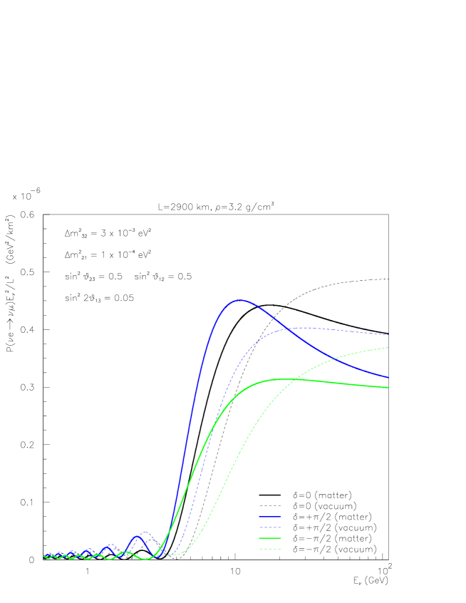
Figure 11: Rescaled probability (see text) for ${\nu_{e}}\rightarrow{\nu_{\mu}}$ oscillations for a baseline $L=2900\ \rm km$ as a function of neutrino energy $E_{\nu}$. The probabilities are computed for neutrinos in matter (full line) and in vacuum (dotted line), and for three values of the $\delta$-phase: $\delta=0$, $\delta=+\pi/2$, $\delta=-\pi/2$. The other oscillation parameters are $\Delta m^{2}_{32}=3\times 10^{-3}\ \rm eV^{2}$, $\Delta m^{2}_{21}=1\times 10^{-4}\ \rm eV^{2}$, $\sin^{2}\theta_{23}=0.5$, $\sin^{2}\theta_{12}=0.5$, $\sin^{2}2\theta_{13}=0.05$.

7 The rescaled probabilities

In order to compare effects at different energies and various baselines, we define a “rescaled probability” parameter that allows a direct comparison of effects. Since to a good approximation, the neutrino energy distribution at the neutrino factory behaves like $E_{\nu}^{2}$ and in addition, the neutrino flux scales like $L^{-2}$ due to the beam divergence, we define the “rescaled probability” parameter $p(\nu_{\alpha}\rightsquigarrow\nu_{\beta};E_{\nu},L)$ as

$$p(\nu_{\alpha}\rightsquigarrow\nu_{\beta};E_{\nu},L)\equiv P(\nu_{\alpha}\rightsquigarrow\nu_{\beta};E_{\nu},L)\times\frac{E^{2}_{\nu}}{L^{2}}$$ (14)

This behaviour is illustrated in Figure 11 for a baseline $L=2900\rm\ km$. We note that (1) it approximately correctly “weighs” the probability by the neutrino energy spectrum $E_{\nu}^{2}$ of the neutrino factory spectrum; (2) it can be directly compared at different baselines, since it contains the $L^{-2}$ attenuation of the neutrino flux with distance $L$; (3) $p$ tends to a constant for $E_{\nu}\rightarrow\inf$, hence the high energy behavior can be easily studied.

8 Propagation in matter

Since neutrino factories will be associated to long baseline, it is not possible to avoid including effects associated to the neutrino propagation through the Earth matter. The simplest way to take into account these effects is to maintain the formalism developed for propagation in vacuum and to replace the mixing angles and the neutrino mass differences by “effective” values.

An important quantity for matter effects is $D$, defined as

$$D(E_{\nu},\rho)\equiv 2\sqrt{2}G_{F}n_{e}E_{\nu}=7.56\times 10^{-5}eV^{2}(\frac{\rho}{gcm^{-3}})(\frac{E_{\nu}}{GeV})$$ (15)

where $n_{e}$ is the electron density and $\rho$ the matter density. For antineutrinos, $D$ is replaced by $-D$.

There are two specific neutrino energies of interest when neutrinos propagate through matter:

1. for $D\approx\Delta m^{2}_{32}$, we reach for neutrinos the MSW resonance, in which the effective mixing angle $\sin^{2}(2\theta^{m}_{13})\approx 1$. In terms of neutrino energy, this implies

   $$E^{res}_{\nu} = \frac{\cos 2\theta_{13}\Delta m^{2}_{32}}{2\sqrt{2}G_{F}n_{e}}={\cal E}^{res}\cos 2\theta_{13}\Delta m^{2}_{32}$$ (16)

   $$\simeq \frac{1.32\times 10^{4}\cos 2\theta_{13}\Delta m^{2}_{32}(\rm eV^{2})}{\rho(g/cm^{3})}\ \rm in\ GeV$$

   where ${\cal E}^{res}=(2\sqrt{2}G_{F}n_{e})^{-1}$. For density parameters $\rho$ equal to $2.7$, $3.2$ and $3.7\rm\ g/cm^{3}$ one finds $E^{res}_{\nu}\simeq 14.1$, $12.3$ and $10.7\rm\ GeV$ for $\Delta m^{2}_{32}=3\times 10^{-3}\rm\ eV^{2}$.

2. for $D>2\Delta m^{2}_{32}$, the effective mixing angle for neutrinos is always smaller than that in vacuum, i.e. $\sin^{2}(2\theta^{m}_{13})<\sin^{2}(2\theta_{13})$. In terms of neutrino energy, this is equivalent to

   $$E_{\nu}>2E^{res}_{\nu}$$ (17)

3. these arguments are independent of the baseline $L$ and depend only on the matter density $\rho$.

9 Detecting the $\delta$ phase at the NF

In order to further study the dependence of the $\delta$-phase, we consider the following three quantities which are good discriminators for a non-vanishing phase $\delta$:

1. $\Delta_{\delta}\equiv P(\nu_{e}\rightarrow\nu_{\mu},\delta=+\pi/2)-P(\nu_{e}\rightarrow\nu_{\mu},\delta=0)$
   The discriminant $\Delta_{\delta}$ can be used in an experiment where one is comparing the measured ${\nu_{e}}\rightarrow{\nu_{\mu}}$ oscillation probability as a function of the neutrino energy $E_{\nu}$ compared to a “Monte-Carlo prediction” of the spectrum in absence of $\delta$-phase.

2. $\Delta_{CP}(\delta)\equiv P(\nu_{e}\rightarrow\nu_{\mu},\delta)-P(\bar{\nu}_{e}\rightarrow\bar{\nu}_{\mu},\delta)$
   The discriminant $\Delta_{CP}$ can be used in an experiment by comparing the appearance of $\nu_{\mu}$ (resp. $\bar{\nu}_{\mu}$) in a beam of stored $\mu^{+}$ (resp. $\mu^{-}$) decays as a function of the neutrino energy $E_{\nu}$.

3. $\Delta_{T}(\delta)\equiv P(\nu_{e}\rightarrow\nu_{\mu},\delta)-P(\nu_{\mu}\rightarrow\nu_{e},\delta)$ or $\bar{\Delta}_{T}(\delta)\equiv P(\bar{\nu}_{e}\rightarrow\bar{\nu}_{\mu},\delta)-P(\bar{\nu}_{\mu}\rightarrow\bar{\nu}_{e},\delta)$
   The discriminant $\Delta_{T}$ can be used in an experiment by comparing the appearance of $\nu_{\mu}$ (resp. $\bar{\nu}_{\mu}$) and $\bar{\nu}_{e}$ (resp. $\nu_{e}$) and in a beam of stored $\mu^{+}$ (resp. $\mu^{-}$) decays as a function of the neutrino energy $E_{\nu}$.

Each of these discriminants have their advantages and disadvantages.

The $\Delta\delta$-method consists in searching for distortions in the visible energy spectrum of events produced by the $\delta$-phase. While this method can in principle provide excellent determination of the phase limited only by the statistics of accumulated events, in practice, systematic effects will have to be carefully kept under control in order to look for a small effect in a seen-data versus Monte-Carlo-expected comparison. In addition, the precise knowledge of the other oscillation parameters will be important, and as will be discussed below, there is a risk of degeneracy between solutions and a possible strong correlation with the $\theta_{13}$ angle at high energy.

The $\Delta_{CP}$ is quite straight-forward, since it involves comparing the appearance of so-called wrong-sign muons for two polarities of the stored muon beam. It really takes advantage from the fact that experimentally energetic muons are rather easy to detect and identify due to their penetrating nature, and with the help of a magnetic field, their change can be easily measured, in order to suppress the non-oscillated background from the beam. A non-vanishing $\Delta_{CP}$ should in principle be a direct proof for a non-vanishing $\delta$-phase. This method suffers, however, from the inability to perform long-baseline experiment through vacuum. Indeed, matter effects will largely “spoil” $\Delta_{CP}$ since it involves both neutrinos and antineutrinos, which will oscillate very differently through matter. Hence, the $\Delta_{CP}$ requires a good understanding of the effects related to matter. In addition, it involves measuring neutrinos and antineutrinos. The matter suppression of the antineutrinos will in practice determine the statistical accuracy with which the discriminant can be measured.

Finally, the $\Delta_{T}$ is the theoretically cleanest method, since it does not suffer from the problems of $\Delta\delta$ and $\Delta_{CP}$. Indeed, a difference in oscillation probabilities between ${\nu_{e}}\rightarrow{\nu_{\mu}}$ and ${\nu_{\mu}}\rightarrow{\nu_{e}}$ would be a direct proof for a non-vanishing $\delta$-phase. In addition, matter affects both probabilities in a same way, since it involves only neutrinos. Unfortunately, it is experimentally very challenging to discriminate the electron charge produced in the events, needed in order to suppress the background from the beam. However, one can decide to measure only neutrinos, which are enhanced by matter effects, as opposed to antineutrinos in the $\Delta_{CP}$ which were matter suppressed, and hence the statistical accuracy of the measurement will be determined by the efficiency to recognize the electron charge, rather by matter suppression.

10 The $L/E_{\nu}$ scaling of the CP and T effects

Regardless of their advantages and disadvantages, there is one thing in common between the three discriminants $\Delta_{\delta}$, $\Delta_{CP}$ and $\Delta_{T}$: their behavior with respect to the neutrino energy $E_{\nu}$ and the baseline $L$. By explicit calculation, we find

$$\Delta_{\delta} = -\frac{1}{2}c^{2}_{13}\sin 2\theta_{12}s_{13}\sin 2\theta_{23}\times$$

$$\Bigl{[}\cos 2\Delta_{13}-\cos 2\Delta_{23}-2\cos 2\theta_{12}\sin^{2}\Delta_{12}+\sin 2\Delta_{12}-\sin 2\Delta_{13}+\sin 2\Delta_{23}\Bigr{]}$$

$$= -\frac{1}{2}c^{2}_{13}s_{13}\Bigl{[}\cos 2\Delta_{13}-\cos 2\Delta_{23}+\sin 2\Delta_{12}-\sin 2\Delta_{13}+\sin 2\Delta_{23}\Bigr{]}$$

where for the second line we assumed for simplicity $\theta_{12}=\theta_{23}=\pi/4$, and similarly,

$$\Delta_{CP}=\Delta_{T} = c^{2}_{13}s_{13}\sin 2\theta_{12}\sin 2\theta_{23}\sin\delta\Bigl{[}\sin 2\Delta_{12}-\sin 2\Delta_{13}+\sin 2\Delta_{23}\Bigr{]}$$ (19)

$$= -c^{2}_{13}s_{13}\sin 2\theta_{12}\sin 2\theta_{23}\sin\delta\Bigl{[}\sin\Delta_{12}\sin\Delta_{13}\sin\Delta_{23}\Bigr{]}$$

As expected, both expressions vanish in the limit $\Delta m^{2}_{12}\rightarrow 0$ where $\Delta m^{2}_{13}\rightarrow\Delta m^{2}_{23}$. Also, as one reaches the higher energies, the terms $\Delta_{CP}=\Delta_{T}$ vanish as

$$|\Delta_{CP}|=|\Delta_{T}| \simeq c^{2}_{13}s_{13}\sin 2\theta_{12}\sin 2\theta_{23}\sin\delta\Delta m^{2}_{12}\left(\frac{L}{4E_{\nu}}\right)\sin^{2}\left(\Delta m^{2}_{23}\frac{L}{4E_{\nu}}\right)$$ (20)

$$\simeq c^{2}_{13}s_{13}\sin 2\theta_{12}\sin 2\theta_{23}\sin\delta\Delta m^{2}_{12}(\Delta m^{2}_{23})^{2}\left(\frac{L}{4E_{\nu}}\right)^{3}$$

hence, in the very high energy limit at fixed baseline, the effects decrease as $E_{\nu}^{-3}$. That the effects disappear at high energy is expected, since in this regime, the “oscillations” of the various $\Delta_{jk}$’s wash out.

The important point is that all expressions depend from some factors which contain the various mixing angles, multiplied by oscillatory terms which always vary like sine or cosine of $\Delta_{jk}$-terms (the terms in squared brackets in the expressions above). Hence, we expect the various discriminants to scale like $\Delta_{jk}\propto L/E_{\nu}$. The sensitivity to the $\delta$-phase will therefore follow the behavior of the oscillation probability, and we therefore argue that the maximum of the effect will occur around the “first maximum” of the oscillations, i.e. for $E^{max}_{\nu}\equiv\Delta m^{2}_{32}L/2\pi$ (see Eq. (13))

These considerations are strictly true only for propagation in vacuum. When neutrinos propagate through matter, matter effects will alter these conclusions. We will however show that as long as the baseline is smaller than some distance such that the corresponding “first maximum” $E^{max}_{\nu}$ lies below the MSW resonance neutrino energy $E^{res}_{\nu}$, the considerations related to the $L/E_{\nu}$ scaling are still largely valid.

In what way does the matter effect alter the ability to look for effects related to the $\delta$-phase? It is incorrect to believe that only the $\Delta_{CP}$ discriminant will be affected by propagation through matter, since it is the only one to a priori mix neutrinos and antineutrinos. In reality, the “dangerous” effect of matter is to reduce the dependence of the probability on the $\delta$-phase, and this for any kind of discriminant.

In matter, we would for example write the $\Delta_{T}$ discriminant as

$$|\Delta^{m}_{T}| = (c^{m}_{13})^{2}s^{m}_{13}\sin 2\theta^{m}_{12}\sin 2\theta^{m}_{23}\sin\delta^{m}\Bigl{[}\sin\Delta^{m}_{12}\sin\Delta^{m}_{13}\sin\Delta^{m}_{23}\Bigr{]}$$ (22)

$$\simeq (c^{m}_{13})^{2}s^{m}_{13}\sin 2\theta^{m}_{12}\sin 2\theta_{23}\sin\delta\Bigl{[}\sin\Delta^{m}_{12}\sin\Delta^{m}_{13}\sin\Delta^{m}_{23}\Bigr{]}$$

where because of our choice of $\Delta m^{2}_{jk}$’s, we have $\theta^{m}_{23}\approx\theta_{23}$ and $\delta^{m}\approx\delta$. This implies that the $\delta$-phase discriminants have a different structure that the terms that define the probability of the oscillation (i.e. the non $\delta$-phase dependent terms). The discriminants are the products of sines and cosines of all mixing angles and of the $\Delta_{jk}$’s (see Eqs. (10) and (19)). Because of this structure, their property in matter is different.

The behavior for neutrino energies above the MSW resonance $E^{res}_{\nu}$ is determined by the fact that in this energy regime, $\theta^{m}_{13}(E>E_{\nu}^{res})\rightarrow\pi/2$ and therefore $c^{m}_{13}\rightarrow 0$ and $s^{m}_{13}\rightarrow 1$. More explicitly, one can show that

$$(c^{m}_{13})^{2}s^{m}_{13} \propto E_{\nu}^{-2}$$

$$\sin 2\theta^{m}_{23} \simeq \sin 2\theta_{23}=const.$$

$$\sin 2\theta^{m}_{12} \rightarrow const.$$

$$\Delta M^{2}_{31} \approx \Delta M^{2}_{32}\propto E_{\nu}$$

$$\Delta M^{2}_{21} \approx \Delta m^{2}_{32}=const$$ (23)

Therefore,

$$|\Delta^{m}_{T}| \propto E_{\nu}^{-2}\sin\delta\Bigl{[}\sin\left(\Delta m^{2}_{32}\frac{L}{4E_{\nu}}\right)\sin^{2}\left(\Delta M^{2}_{13}\frac{L}{4E_{\nu}}\right)\Bigr{]}\propto E_{\nu}^{-3}$$ (24)

and one recovers a neutrino energy dependence identical to that in vacuum (see Eq. (20)). Note also that the argument of the sine function $\Delta M^{2}_{13}L/4E_{\nu}$ is not small (i.e. the approximation $\sin x\simeq x$ is not valid). For our choice of oscillation parameters, the mass difference is approximately equal to $\Delta M^{2}_{13}(\rm eV^{2})\simeq 3\times 10^{-4}\times E_{\nu}(\rm GeV)$, and hence the dependence on the baseline is

$$|\Delta^{m}_{T}| \propto E_{\nu}^{-2}\sin\delta\Bigl{[}\sin\left(1.27\Delta m^{2}_{32}\frac{L(\rm km)}{E_{\nu}(\rm GeV)}\right)\sin^{2}\left(3.8\times 10^{-4}L(\rm km)\right)\Bigr{]}$$ (25)

Hence, the discriminant will first be enhanced and then be suppressed by matter effects. The maximum is found when the sine squared function reaches a maximum, or at approximately 4000 km under the assumption of high energy neutrinos.

As anticipated, these discussions say that if one wants to study oscillations in the region of the “first maximum”, one should not choose a too large baseline $L$, otherwise, matter effects will suppress the oscillation probability. This is even more so true, as it will be recalled below, that the magnitude of the effects related to the $\delta$-phase are suppressed more rapidly than the oscillation.

The simplest way to express the condition on the matter is to require that the energy of the “first maximum” be smaller than the MSW resonance energy:

$$2\sqrt{2}G_{F}n_{e}E^{max}_{\nu}\lesssim\Delta m^{2}_{32}\cos 2\theta_{13}$$ (26)

and, by inserting the definition of $E^{max}_{\nu}\equiv\Delta m^{2}_{32}L/2\pi$ we get

$$L_{max} \lesssim \frac{\pi\cos 2\theta_{13}}{\sqrt{2}G_{F}n_{e}}\approx\frac{\pi\cos 2\theta_{13}}{2\times 1.27\times 7.56\times 10^{-5}(\rm eV^{2})\rho(\rm g/cm^{3})}$$ (27)

$$\approx \frac{1.5\times 10^{4}(\rm km)}{\rho(\rm g/cm^{3})}\approx 5000\rm\ km$$

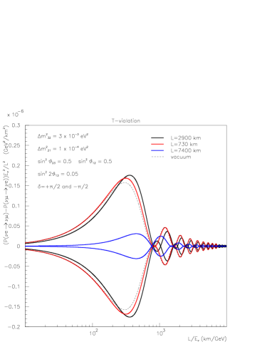
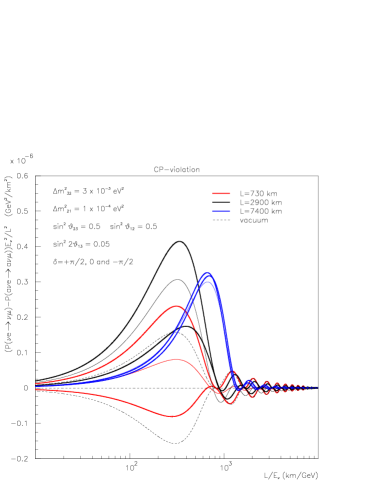
Figure 12: The rescaled $\Delta_{T}$ and $\Delta_{CP}$ discriminants (see text for definition) as a function of the $L/E_{\nu}$ ratio, computed for neutrinos propagating in matter at three different baselines $L=730\rm\ km$, 2900 km and 7400 km, and also for propagation vacuum (independent of baseline). Three sets of curves are represented, corresponding to $\delta=+\pi/2$ and $\delta=-\pi/2$ (thick lines) and $\delta=0$ (thin lines). The other oscillation parameters are $\Delta m^{2}_{32}=3\times 10^{-3}\ \rm eV^{2}$, $\Delta m^{2}_{21}=1\times 10^{-4}\ \rm eV^{2}$, $\sin^{2}\theta_{23}=0.5$, $\sin^{2}\theta_{12}=0.5$ and $\sin^{2}2\theta_{13}=0.05$.

To summarize, we find that the discriminants of the $\delta$-phase all scale with $L/E_{\nu}$. This is illustrated in Figure 12, where the rescaled $\Delta_{T}$ and $\Delta_{CP}$ discriminants are plotted as a function of the $L/E_{\nu}$ ratio. In the plots, sets of curves are shown for $\delta=+\pi/2$ and $\delta=-\pi/2$. We see that the rescaled $T$-discriminant is (as expected) antisymmetric with respect to $\delta$. For the shorter baselines (730 km and 2900 km) it is almost equivalent to the vacuum case (dashed curves). The 7400 km baseline yields a highly suppressed $T$-effect. The $CP$-discriminant has the same features, but is shifted with respect to zero due to matter enhancement.

The most favorable choice of neutrino energy $E_{\nu}$ and baseline $L$ is in the region of the “first maximum” given by $(L/E_{\nu})^{max}\simeq 400$ for $|\Delta m^{2}_{32}|=3\times 10^{-3}\rm\ eV^{2}$. This leaves a great flexibility in the choice of the actual neutrino energy and the baseline, since only their ratio $L/E_{\nu}$ is determinant.

Because of the rising neutrino cross-section with energy, it will be more favorable to go to higher energies if the neutrino fluence is constant. Keeping the $L/E_{\nu}$ ratio constant, this implies an optimization at longer baselines $L$. One will hence gain with the baseline $L$ until we reach $L_{max}\approx 5000\rm\ km$ beyond which matter effects will effectively reduce the dependence of the oscillation probabilities on the $\delta$-phase.

11 The correlation with $\theta_{13}$

We begin the discussion with the detection of the $\delta$-phase with the method of the $\Delta_{\delta}$ discriminant. We recall that this method implies the comparison of the measured ${\nu_{e}}\rightarrow{\nu_{\mu}}$ oscillation probability as a function of the neutrino energy $E_{\nu}$ compared to a “Monte-Carlo prediction” of the spectrum in absence of $\delta$-phase.

When searching for effects related to the $\delta$-phase by comparing the measured ${\nu_{e}}\rightarrow{\nu_{\mu}}$ oscillation probability as a function of the neutrino energy $E_{\nu}$ to a “Monte-Carlo prediction” of the spectrum in absence of $\delta$-phase, requires necessarily a precise knowledge of the other oscillation parameters entering in the oscillation probability expression.

In particular, the knowledge of the angle $\theta_{13}$ could be quite important. Indeed, the ${\nu_{e}}\rightarrow{\nu_{\mu}}$ oscillation is primarily driven by the $\theta_{13}$ angle and only thanks to a different energy dependence of the terms proportional to $\delta$ than to those independent of $\delta$ can one hope to determine $\theta_{13}$ and $\delta$ at the same time!

This is however not true at high energy, when both $|\Delta_{12}|\ll 1$ and $|\Delta_{13}|,|\Delta_{23}|\ll 1$. This can be explicitly shown for example for simplicity in the limit of small $\theta_{13}$. The rescaled probability is in this case a constant:

$$p(\nu_{e}\rightarrow\nu_{\mu}) \simeq \frac{(\Delta m^{2}_{12})^{2}}{32}\Bigl{\{}1+2Ms^{2}_{13}+8Ns_{13}\cos\delta\Bigr{\}}$$ (28)

where $M=((\Delta m^{2}_{13})^{2}+(\Delta m^{2}_{23})^{2})/(\Delta m^{2}_{12})^{2}$ and $N=(\Delta m^{2}_{13}+\Delta m^{2}_{23})/(\Delta m^{2}_{12})$. The absence of “oscillations” at high energy implies that a change of $\theta_{13}$ can mimic a change of $\delta$. In practice, this implies that the best energy range to look for effects related to the $\delta$-phase is close the “first oscillation maximum”, i.e. $E^{max}_{\nu}\simeq 2\rm\ GeV$ at 730 km or $E^{max}_{\nu}\simeq 8\rm\ GeV$ at 2900 km. This implies that the detector should be able to reconstruct neutrino events at those energies with high efficiency, and low background.

12 Two concrete examples at L=730 km and 2900 km

In order to assess with concrete examples the use of the $\delta$-phase discriminants, we consider the two baselines, with corresponding muon beam energy:

• $L$=732 km, $E_{\mu}=7.5\rm\ GeV$, $10^{21}$ muon decays

• $L$=2900 km, $E_{\mu}=30\rm\ GeV$, $2.5\times 10^{20}$ muon decays

Both examples were chosen to have the same $L/E_{\mu}$. Because of the linear rise of the neutrino cross-section with $E_{\nu}$, the factor 4 in muon energy between the 732 km and 2900 km case, is “compensated” by an increase of intensity by the same factor in favor of the shorter baseline.

The expected event rates are shown in Tables 1 and 2.

		$E_{\mu}=7.5\rm\ GeV$	$E_{\mu}=30\rm\ GeV$
	Process	$L=732\rm\ km$	$L=2900\rm\ km$
		$10^{21}$ $\mu^{-}$	$2.5\times 10^{20}$ $\mu^{-}$
	$\nu_{\mu}$ CC	41690	36050
Non-oscillated	$\nu_{\mu}$ NC	10700	10300
rates	$\bar{\nu}_{e}$ CC	14520	13835
	$\bar{\nu}_{e}$ NC	4266	4975
Oscillated	$\bar{\nu}_{e}\rightsquigarrow\bar{\nu}_{\mu}$ CC	88	50
events ($\delta=\pi/2$)	$\nu_{\mu}\rightsquigarrow\nu_{e}$ CC	258	238
Oscillated	$\bar{\nu}_{e}\rightsquigarrow\bar{\nu}_{\mu}$ CC	100	54
events ($\delta=0$)	$\nu_{\mu}\rightsquigarrow\nu_{e}$ CC	385	333
Oscillated	$\bar{\nu}_{e}\rightsquigarrow\bar{\nu}_{\mu}$ CC	100	55
events ($\delta=-\pi/2$)	$\nu_{\mu}\rightsquigarrow\nu_{e}$ CC	376	330

Table 1: Event rates for a 10 kton detector. The oscillation parameters are: $\Delta m_{32}^{2}=3\times 10^{-3}\rm\ eV^{2}$, $\Delta m^{2}_{12}=1\times 10^{-4}\rm\ eV^{2}$, $\sin^{2}\theta_{23}=0.5$, $\sin^{2}\theta_{12}=0.5$ and $\sin^{2}2\theta_{13}=0.05$.

		$E_{\mu}=7.5\rm\ GeV$	$E_{\mu}=30\rm\ GeV$
	Process	$L=732\rm\ km$	$L=2900\rm\ km$
		$10^{21}$ $\mu^{+}$	$2.5\times 10^{20}$ $\mu^{+}$
	$\bar{\nu}_{\mu}$ CC	16570	15962
Non-oscillated	$\bar{\nu}_{\mu}$ NC	5096	5600
rates	$\nu_{e}$ CC	37570	32100
	$\nu_{e}$ NC	9143	9175
Oscillated	$\nu_{e}\rightsquigarrow\nu_{\mu}$ CC	445	397
events ($\delta=\pi/2$)	$\bar{\nu}_{\mu}\rightsquigarrow\bar{\nu}_{e}$ CC	86	46
Oscillated	$\nu_{e}\rightsquigarrow\nu_{\mu}$ CC	438	387
events ($\delta=0$)	$\bar{\nu}_{\mu}\rightsquigarrow\bar{\nu}_{e}$ CC	86	45
Oscillated	$\nu_{e}\rightsquigarrow\nu_{\mu}$ CC	289	277
events ($\delta=-\pi/2$)	$\bar{\nu}_{\mu}\rightsquigarrow\bar{\nu}_{e}$ CC	77	42

Table 2: Same as Table 1, but $\mu^{+}$ decays.

12.1 Direct extraction of the oscillation probabilities

From the visible energy distributions of the events, one can extract the oscillation probabilities. The visible energy of the events are plotted into histograms with 10 bins in energy. The ${\nu_{e}}\rightarrow{\nu_{\mu}}$ oscillation probability in each energy bin $i$ can be computed as

$${\cal P}_{i}({\nu_{e}}\rightarrow{\nu_{\mu}})=\frac{N_{i}(ws\mu)-N^{0}_{i}(ws\mu)}{\epsilon_{i}(p_{\mu}>p_{\mu}^{cut})N_{i}^{0}(e)}$$ (29)

where $N_{i}(ws\mu)$ is the number of wrong-sign muon events in the i-th bin of energy, $N^{0}_{i}(ws\mu)$ are the background events in the i-th bin of energy, $\epsilon_{i}(p_{\mu}>p_{\mu}^{cut})$ is the efficiency of the muon threshold cut in that bin, and $N_{i}^{0}(e)$ is the number of electron events in the i-th bin of energy in absence of oscillations. The number of events corresponds to the statistics obtained from $\mu^{+}$ decays. A similar quantity for antineutrinos ${\cal P}_{i}(\bar{\nu_{e}}\rightarrow\bar{\nu_{\mu}})$ will be computed with events coming from $\mu^{-}$ decays.

Similarly, the ${\nu_{\mu}}\rightarrow{\nu_{e}}$ oscillation probability in each energy bin $i$ can be computed as

$${\cal P}_{i}({\nu_{\mu}}\rightarrow{\nu_{e}})=\frac{N_{i}(wse)-N^{0}_{i}(wse)}{\epsilon_{e}(1-p_{conf})N_{i}^{0}(rs\mu)}$$ (30)

where $N_{i}(wse)$ is the number of wrong-sign electron events in the i-th bin of energy, $\epsilon_{e}$ is the efficiency for charge discrimination, $p_{conf}$ the charge confusion, and $N_{i}^{0}(rs\mu)$ is the number of right sign muon events in the i-th bin of energy in absence of oscillations. The number of events corresponds to the statistics obtained from $\mu^{-}$ decays. A similar quantity for antineutrinos ${\cal P}_{i}(\bar{\nu_{\mu}}\rightarrow\bar{\nu_{e}})$ will be computed with events coming from $\mu^{+}$ decays.

These binned probabilities could be combined in an actual experiment in order to perform direct searches of the effects induced by the $\delta$-phase.

12.2 Direct search for T-asymmetry

For measurements involving the discrimination of the electron charge, we limit ourselves to the lowest energy and baseline configuration ($E_{\mu}=7.5\rm\ GeV$ and $L=732\rm\ km$), since we expect the discrimination of the electron charge to be practically possible only at these lowest energies.

The binned $\Delta_{T}(i)$ discriminant for neutrinos is defined as

$$\Delta_{T}(i)={\cal P}_{i}({\nu_{\mu}}\rightarrow{\nu_{e}})-{\cal P}_{i}({\nu_{e}}\rightarrow{\nu_{\mu}})$$ (31)

and a similar discriminant $\bar{\Delta}_{T}(i)$ can be computed for antineutrinos.

These quantities are plotted for neutrinos and antineutrinos for three values of the $\delta$-phase ($\delta=+\pi/2$, $\delta=0$ and $\delta=-\pi/2$) in Figure 13. The errors are statistical and correspond to a normalization of $10^{21}$ muon decays and a baseline of $L=732\rm\ km$. A 20% electron efficiency with a charge confusion probability of 0.1% has been assumed. The full curve corresponds to the theoretical probability difference.

A nice feature of these measurements is the change of sign of the effect with respect of the change $\delta\rightarrow-\delta$ and also with respect to the substitution of neutrinos by antineutrinos. These changes of sign are clearly visible and would provide a direct, model-independent, proof for T-violation in neutrino oscillations.

In order to cross-check the matter behavior, one can also contemplate the $CPT$-discriminants defined as

$$\Delta_{CPT}(i)={\cal P}_{i}({\nu_{\mu}}\rightarrow{\nu_{e}})-{\cal P}_{i}(\bar{\nu_{e}}\rightarrow\bar{\nu_{\mu}})$$

$$\bar{\Delta}_{CPT}(i)={\cal P}_{i}({\nu_{e}}\rightarrow{\nu_{\mu}})-{\cal P}_{i}(\bar{\nu_{\mu}}\rightarrow\bar{\nu_{e}})$$ (32)

These quantities are independent from the $\delta$-phase and probe only the matter effects. The change of sign of the effect with respect to the substitution of neutrinos by antineutrinos is clearly visible.

It should be however noted that in the case of the $CPT$ discriminant, the statistical power is rather low, since this measurement combines the appearance of electrons (driven by the efficiency for detecting the electron charge) and involves antineutrinos, which are suppressed by matter effects. Hence, the statistical power is reduced compared to the $T$-discriminant.

12.3 Direct search for CP-asymmetry

In the direct search for the CP-asymmetry, we rely only on the appearance of wrong-sign muons. We compare in this case the two energy and baselines options.

The binned $\Delta_{CP}(i)$ discriminant for the shortest baseline $L=732\rm\ km$, $E_{\mu}=7.5\rm\ GeV$ and longest baseline $L=2900\rm\ km$, $E_{\mu}=30\rm\ GeV$ (lower plots) for three values of the $\delta$-phase ($\delta=+\pi/2$, $\delta=0$ and $\delta=-\pi/2$) are shown in Figure 13. The errors are statistical and correspond to a normalization of $10^{21}$($2.5\times 10^{20}$) for $L=732(2900)\rm\ km$. The full curve corresponds to the theoretical probability difference. The dotted curve is the theoretical curve for $\delta=0$ and represents the effect of propagation in matter.

As was already pointed out, the $\Delta_{CP}$ does not vanish even in the case $\delta=0$, since matter traversal introduces an asymmetry. At the shortest baseline ($L=732\rm\ km$), these effects are rather small. This has the advantage that the observed asymmetry would be positive for $\delta>0$, but would still change sign in the case $\delta\approx-\pi/2$. In the fortunate case in which Nature has chosen such a value for the $\delta$-phase, the observation of the negative asymmetry would be a striking sign for CP-violation, since matter could never produce such an effect.

For other values of the $\delta$-phase, the effect is positive. It is also always positive at the largest baseline $L=2900\rm\ km$, since at those distances the effect induced by the $\delta$-phase is smaller than the asymmetry introduced by the matter.

12.4 Comparison of two methods

The binned $\Delta_{T}(i)$ and $\Delta_{CP}(i)$ discriminant can be used to calculate the $\chi^{2}$ significance of the effect, given the statistical error on each bin. We compute the following $\chi^{2}$’s:

$$\chi^{2}_{T}=\sum_{i}\frac{\left(\Delta_{T}(i,\delta)-\Delta_{T}(i,\delta=0)\right)^{2}}{\sigma(\Delta_{T}(i,\delta))^{2}}+\frac{\left(\bar{\Delta}_{T}(i,\delta)-\bar{\Delta}_{T}(i,\delta=0)\right)^{2}}{\sigma(\bar{\Delta}_{T}(i,\delta))^{2}}$$ (33)

where $\sigma(\Delta_{T}(i,\delta))$ is the statistical error in the bin. Similarly, the $\chi^{2}$ of the CP-asymmetry is

$$\chi^{2}_{CP}=\sum_{i}\frac{\left(\Delta_{CP}(i,\delta)-\Delta_{CP}(i,\delta=0)\right)^{2}}{\sigma(\Delta_{CP}(i,\delta))^{2}}$$ (34)

We study the significance of the effect as a function of the solar mass difference $\Delta m^{2}_{21}$, since the effect associated to the $\delta$-phase will decrease with decreasing $\Delta m^{2}_{21}$ values. We consider the range compatible with solar neutrino experiments, $10^{-5}\lesssim\Delta m^{2}_{21}\lesssim 10^{-4}\rm\ eV^{2}$.

The exclusion regions obtained at the 90%C.L. (defined as $\Delta\chi^{2}=+1.96$) in the $\delta$-phase vs $\Delta m^{2}_{21}$ plane are shown in Figure 14. A 20% electron efficiency with a charge confusion probability of 0.1% has been assumed. The normalizations assumed are $10^{21}$ and $5\times 10^{21}$ muon decays with energy $E_{\mu}=7.5\rm\ GeV$ and a baseline of $L=732\rm\ km$.

The results are very encouraging. With $10^{21}$ muon decays, the region $\Delta m^{2}_{21}\gtrsim 5\times 10^{-5}\rm\ eV^{2}$ is covered. For $5\times 10^{21}$ muons, this region extends down to $10^{-5}\rm\ eV^{2}$, in order words, the full range of values compatible with the LMA solar data is testable.

Figure 13: Direct T- and CP-violation: Binned $\Delta_{T}(i)$(left) and $\Delta_{CP}(i)$(right) discriminants for neutrinos (upper plots) and antineutrinos (lower plots) for three values of the $\delta$-phase: $\delta=+\pi/2$, $\delta=0$ and $\delta=-\pi/2$. The errors are statistical and correspond to the normalizations given in the text. A 20% electron efficiency with a charge confusion probability of 0.1% has been assumed. The full curve corresponds to the theoretical probability difference.

If we consider that the value of $\Delta m^{2}_{21}$ is known and that it has a value of $\Delta m^{2}_{21}=10^{-4}\rm\ eV^{2}$, one can constrain the values of the $\delta$-phase within the range $|\delta|\lesssim 0.35$ or $|\delta|\gtrsim 2.8$ for $10^{21}$ muons and $|\delta|\lesssim 0.14$ for $5\times 10^{21}$ muon decays at the 90%C.L. We conclude that an exhaustive direct, model-independent exploration of the $\delta$-phase, within the full range $10^{-5}\lesssim\Delta m^{2}_{21}\lesssim 10^{-4}\rm\ eV^{2}$ requires an intensity of $5\times 10^{21}$ muon decays of each sign.

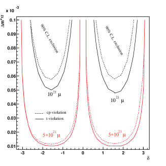
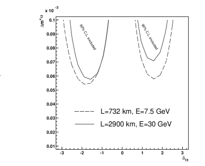
Figure 14: Exclusion region at the 90%C.L. in the $\delta$-phase vs $\Delta m^{2}_{21}$ plane. Two regions obtained with the $\Delta_{T}$ and $\Delta_{CP}$ discriminants are shown. A 20% electron efficiency with a charge confusion probability of 0.1% has been assumed. The normalization is $10^{21}(5\times 10^{21})$ muon decays with energy $E_{\mu}=7.5\rm\ GeV$ and a baseline of $L=732\rm\ km$.

13 Conclusion

We argued that the ideal neutrino detector at the neutrino factory should (1) have a mass in the range of 10 kton, (2) provide particle identification to tag the flavor of the incoming neutrino, (3) lepton charge measurement to select the incoming neutrino helicity, (4) good energy resolution to reconstruct the incoming neutrino energy, (5) possess a low energy threshold, in order to study neutrino events in the energy region where $CP$ and $T$ effects are the cleanest and most unambiguous (see Section 11) and (6) be isotropic to equally well reconstruct incoming neutrinos from different baselines (it might be more efficient to build various sources at different baselines, than various detectors).

A detector with such qualities is most adapted to fully explore neutrino oscillations at the neutrino factory. In particular, measurement of the leading muons and electrons charge is the only way to fully simultaneously study $CP$ and $T$ violation effects.

We think that a magnetized liquid argon imaging detector, scaled to 10 ktons, stands as the best choice of technique which holds the highest hope to match the above mentioned detector requirements.

Such a detector could measure very precisely all the magnitudes of the elements of the mixing matrix and over-constrain them, because of its ability to reconstruct all final states including muons, electrons, tau-like and neutral current events (see Ref.[11]).

In addition, this detector could address the more challenging and most interesting goal of the neutrino factory, which is the search for effects related to the complex phase of the mixing matrix. This is because it could reconstruct the charge of both electrons and muons, and because it is perfectly adapted to reconstruct low energy events (typ. below 15 GeV), which is the energy region where we expect these effects to be the cleanest and the most unambiguous.

The choice of baseline and muon ring energy is in this context particularly critical. In view of the existence of massive devices like SuperK, MINOS or ICARUS, it is also worth considering if these detectors at their current baselines could be reused in the context of the neutrino factory. If new sites have to be found in order to satisfy the requirements of longer baselines, major new “investments” will be required.

We find that the most favorable choice of neutrino energy $E_{\nu}$ and baseline $L$ is in the region of the “first maximum” given by $(L/E_{\nu})^{max}\simeq 400$ for $|\Delta m^{2}_{32}|=3\times 10^{-3}\rm\ eV^{2}$. This yields $E^{max}_{\nu}\simeq 2\rm\ GeV$ at 730 km, $E^{max}_{\nu}\simeq 8\rm\ GeV$ at 2900 km and $E^{max}_{\nu}\simeq 20\rm\ GeV$ at 7400 km for $\Delta m^{2}_{32}=3\times 10^{-3}\rm\ eV^{2}$.

We showed that the discriminants of the $\delta$-phase all scale with $L/E_{\nu}$. This property leaves flexibility in the choice of the actual neutrino energy and the baseline, since only their ratio $L/E_{\nu}$ is determinant. Because of the rising neutrino cross-section with energy, it will be more favorable to go to higher energies if the neutrino fluence is constant. Keeping the $L/E_{\nu}$ ratio constant, this implies an optimization at longer baselines $L$. One will hence gain with the baseline $L$ until we reach $L_{max}\approx 5000\rm\ km$ beyond which matter effects will effectively reduce the dependence of the oscillation probabilities on the $\delta$-phase.

As far as the neutrino energy is concerned, it is clear that the average neutrino energy $E_{\nu}$ scales linearly with the muon beam energy $E_{\mu}$. A non-negligible aspect of the neutrino factory is the need to accelerate quickly the muons to the desired energy, and so, it is expected that higher energies will be more demanding that lower ones. Eventually, cost arguments could determine the muon energy. It could therefore be that lower energy, more intense neutrino factories could be more advantageous than higher energy, less intense ones.

From the above arguments, we therefore conclude that a very intense neutrino factory, capable of providing more than $10^{21}$ useful 7.5 GeV muon decays, directed towards a distance of 730 km, coupled with a magnetized liquid argon imaging detector of about 10 kton would provide the ultimate, most comprehensive setup to study $CP$ and $T$ violation effects in neutrino flavor oscillation.

14 Acknowledgments

I thank Milla Baldo Ceolin for the invitation to the Neutrino Telescope Workshop in the beautiful city of Venice. The help of M. Campanelli and also of A. Bueno is greatly acknowledged.

References

-
[1]
“E362 Proposal for a long baseline neutrino oscillation experiment,
using KEK-PS and Super-Kamiokande”, February 1995.
H. W. Sobel, proceedings of Eighth International Workshop on Neutrino Telescopes, Venice 1999, vol 1 pg 351. - [2] E. Ables et al. [MINOS Collaboration], “P-875: A Long baseline neutrino oscillation experiment at Fermilab,” FERMILAB-PROPOSAL-P-875.
- [3] A. Ereditato, K. Niwa and P. Strolin, INFN/AE-97/06 and Nagoya DPNU-97-07, 27 January 1997, unpublished.
- [4] ICARUS Collaboration, Laboratori Nazionali del Gran Sasso (LNGS) Int. Note, LNGS - 94/99 (Vols I-II), unpublished; LNGS 95/10, unpublished. P. Benetti et al., Nucl. Instrum. Methods A 327, 173 (1993);Nucl. Instrum. Methods A 332, 395 (1993); P. Cennini et al., Nucl. Instrum. Methods A 333, 567 (1993);Nucl. Instrum. Methods A 345, 230 (1994); Nucl. Instrum. Methods A 355, 660 (1995).
- [5] F. Arneodo et al. [ICARUS collaboration], hep-ex/0103008.
- [6] B. Pontecorvo, J. Expt. Theor. Phys. 33, 549 (1957) [Sov. Phys. JETP 6, 429 (1958)]; B. Pontecorvo, J. Expt. Theor. Phys. 34, 247 (1958) [Sov. Phys. JETP 7, 172 (1958)]; Z. Maki, M. Nakagawa and S. Sakata, Prog. Theor. Phys. 28 (1962) 870; B. Pontecorvo, J. Expt. Theor. Phys 53 (1967) 1717; V. Gribov and B. Pontecorvo, Phys. Lett. B 28, 493 (1969).
- [7] Y. Fukuda et al. (Kamiokande Collaboration), Phys. Lett. B 335, 237 (1994); R. Becker-Szendy et al. (IMB Collaboration), Nucl. Phys. B (Proc. Suppl.) 38, 331 (1995); S. Fukuda et al. (Super-Kamiokande Collaboration), hep-ex/0009001; T. Kajita (Super-Kamiokande Collaboration), Talk presented at NOW2000, Otranto, Italy, September 2000 (http://www.ba.infn.it/~now2000); W.W.M. Allison et al. (Soudan 2 Collaboration), Phys. Lett. B 449, 137 (1999); F. Ronga (MACRO Collaboration), Talk presented at NOW2000, Otranto, Italy, September 2000 (http://www.ba.infn.it/~now2000).
- [8] S. Geer, Phys. Rev. D 57, 1998 (6989)
- [9] Information on the neutrino factory studies and mu collider collaboration at BNL can be found at http://www.cap.bnl.gov/mumu/. Information on the neutrino factory studies at FNAL can be found at http://www.fnal.gov/projects/muon_collider/. Information on the neutrino factory studies at CERN can be found at http://muonstoragerings.cern.ch/Welcome.html/.
- [10] A. de Rújula, M. B. Gavela and P. Hernández, Nucl. Phys. B 547, 1999 (21); V. Barger, S. Geer, R. Raja and K. Whisnant, Phys. Rev. D62, 013004 (2000) [hep-ph/9911524]; Phys. Rev. D62, 073002 (2000) [hep-ph/0003184]; A. Bueno, M. Campanelli and A. Rubbia, Nucl. Phys. B573 (2000) 27; V. Barger, S. Geer and K. Whisnant, Phys. Rev. D 61, 2000 (053004); M. Freund, M. Lindner, S. T. Petcov and A. Romanimo, Nucl. Phys. B578, 27 (2000) [hep-ph/9912457]; A. Cervera et al., Nucl. Phys. B579, 17 (2000) [hep-ph/0002108].
- [11] A. Bueno, M. Campanelli and A. Rubbia, Nucl. Phys. B 589, 577 (2000) [hep-ph/0005007].
- [12] J. Arafune, M. Koike and J. Sato, Phys. Rev. D 56, 3093 (1997) [hep-ph/9703351].
- [13] J. Sielaff [DONUT Collaboration], hep-ex/0105042.
- [14] C. K. Jung, Feasibility of a next generation underground water Cherenkov detector: UNO, NNN99 at Stony Brook, hep-ex/0005046.
- [15] C. Rubbia, private communication.
- [16] F. Sergiampietri, NUFACT’01, Tsukuba (Japan), May 2001.