MSW effect for large mixing angles

Alexander Friedland

School of Natural Sciences, Institute for Advanced Study, Princeton, New Jersey 08540

1 Introduction

The MSW mechanism [1, 2, 3] of neutrino flavor oscillations is a simple and very beautiful idea. The effect arises because of the coherent forward scattering of the neutrinos on electrons and nucleons in matter. This scattering makes the “neutrino index of refraction” of the media slightly different from one. The remarkable fact is that this small (and otherwise unobservable) change of the index of refraction can have a dramatic effect on the oscillation probability of solar neutrinos. In particular, when the flavor off-diagonal terms in the neutrino Hamiltonian are small compared to the diagonal terms in vacuum, the flavor conversion can be almost complete.

It is this possibility of the almost complete conversion that initially attracted a lot of attention. The phenomenon was understood as a resonance effect. The flavor conversion was shown to occur at the depth in the Sun where the density is such that the matter effects cancel the difference between the diagonal terms in the neutrino Hamiltonian.

The recent data [4, 5, 6, 7], however, together with the latest solar model [8], indicate that the preferred value of the mixing angle may be large. It was recently emphasized [9] that the resonance picture breaks down in this case. It was shown that the important physical processes, level jumping or flavor conversion, do not occur at the resonance. The correct picture is to consider adiabatic or nonadiabatic neutrino evolution which reduces to the resonance description in the limit $\theta\ll 1$. It is also worth pointing out that this description is perfectly continuous across the point of the maximal mixing $\theta=\pi/4$.

In this note we review these developments. The aim is to keep the presentation as simple as possible, in accordance with the stated goals of the Workshop to make the Proceedings into a pedagogical resource. In Section 2 we present an elementary introduction to the resonance phenomenon. In Section 3 we pose several questions that seem to be difficult to answer within the resonance picture. In Section 4 present the resolutions.

2 Neutrino oscillations and the MSW effect

Let us begin by summarizing the standard treatment of neutrino oscillations. This introduction is not meant to be exhaustive. In fact, quite often the best presentations of any idea are written by people who discovered it or contributed early on, and the case at hand is no exception, see, e.g., [10, 11, 12, 13, 14].

2.1 Simple vacuum oscillations

Suppose at some point one creates the electron neutrino state, for example as a result of a nuclear reaction. Suppose further that there is a term in the Hamiltonian coupling the electron neutrino to some other neutrino state. Then, as the neutrino propagates in vacuum, it will be (partially) converted into that state. Still later, the state will again be $\nu_{e}$ and so on, i. e., the flavor oscillations will take place.

The simplest case is the case of two flavors. The oscillations occur between the electron neutrino $\nu_{e}$ and another active neutrino state, conventionally labeled $\nu_{\mu}$. The Schrödinger equation for this system is

$$i\frac{d}{dt}\left(\begin{array}[]{c}\phi_{e}\\ \phi_{\mu}\end{array}\right)=\left(\begin{array}[]{cc}H_{ee}&H_{e\mu}\\ H_{\mu e}&H_{\mu\mu}\end{array}\right)\left(\begin{array}[]{c}\phi_{e}\\ \phi_{\mu}\end{array}\right).$$ (1)

The presence of the off-diagonal coupling $H_{e\mu}=H_{\mu e}$ ensures that the mass eigenstates $|\nu_{1,2}\rangle$ of this system are not the same as the flavor eigenstates $|\nu_{e,\mu}\rangle$:

$$|\nu_{1}\rangle = \cos\theta|\nu_{e}\rangle-\sin\theta|\nu_{\mu}\rangle,$$

$$|\nu_{2}\rangle = \sin\theta|\nu_{e}\rangle+\cos\theta|\nu_{\mu}\rangle.$$ (2)

Thus, introducing the off-diagonal term in Eq. (1) is equivalent to saying that the mass and flavor eigenstates in the lepton sector are not aligned. We know this is the case in the quark section, where the two bases are related by the CKM matrix, hence it is not unreasonable to expect the misalignment also in the lepton sector.

The coupling $H_{e\mu}$ leads to flavor oscillations as the neutrino state propagates in space. If at $x=0$ the state was purely $\nu_{e}$, after propagating in vacuum to $x=L$ it will be measured as $\nu_{\mu}$ with the probability

$$P(\nu_{e}\rightarrow\mu_{\mu})=\sin^{2}2\theta\sin^{2}\left(\frac{\Delta}{2}L\right).$$ (3)

Here $\Delta$ is one half of the mass splitting, $\Delta\equiv\sqrt{H_{e\mu}^{2}+(H_{\mu\mu}-H_{ee})^{2}/4}=\Delta m^{2}/2E_{\nu}$. Clearly, $\Delta\sin 2\theta=H_{e\mu}$, $\Delta\cos 2\theta=(H_{\mu\mu}-H_{ee})/2$. Since all oscillation phenomena depend only on $(H_{\mu\mu}-H_{ee})/2$ and not on $H_{\mu\mu}$ or $H_{ee}$ separately, we shall often drop the constant term in the Hamiltonian

$$H = \frac{H_{\mu\mu}+H_{ee}}{2}+\left(\begin{array}[]{cc}-(H_{\mu\mu}-H_{ee})/2&H_{e\mu}\\ H_{\mu e}&(H_{\mu\mu}-H_{ee})/2\end{array}\right)$$ (6)

$$\longrightarrow \left(\begin{array}[]{cc}-(H_{\mu\mu}-H_{ee})/2&H_{e\mu}\\ H_{\mu e}&(H_{\mu\mu}-H_{ee})/2\end{array}\right)=\left(\begin{array}[]{rr}-\Delta\cos 2\theta&\Delta\sin 2\theta\\ \Delta\sin 2\theta&\Delta\cos 2\theta\end{array}\right).$$ (11)

2.2 The resonance and the MSW effect

2.2.1 Matter effects

The above picture describes the evolution of the neutrino state in vacuum. One might be tempted to also use the same formulas for the evolution in matter. Indeed, it might seem that the presence of matter has no effect on the neutrino evolution. After all, the scattering cross section for the electron neutrino $\sigma\sim G_{F}^{2}E_{\rm c.m.}^{2}$ is so small for solar neutrinos ($E_{\rm lab}\sim(0.2-15)$ MeV), that the vast majority of them go right through the Sun undeflected.

Nevertheless, the presence of matter does affect the neutrino evolution in an important way. Since the medium is transparent to neutrinos, it is helpful to think in the language of “neutrino optics”. The presence of the medium can lead to a index of refraction for the neutrinos. Since the index of refraction is a phase phenomenon – it is related to the amplitude of the coherent forward scattering – the effect involves the first power of $G_{F}$. Wolfenstein pointed out [1] that this coherent forward scattering leads to the addition of the extra terms to the diagonal elements of the Hamiltonian, $\sqrt{2}G_{F}(N_{e}-N_{n}/2)$ for the electron neutrinos and $\sqrt{2}G_{F}(-N_{n}/2)$ for the other active species. Thus,

$$H_{\rm mat}={\rm const}+\left(\begin{array}[]{cc}A-\Delta\cos 2\theta&\Delta\sin 2\theta\\ \Delta\sin 2\theta&\Delta\cos 2\theta-A\end{array}\right)$$ (12)

where $A\equiv G_{F}N_{e}/\sqrt{2}$. The effect of the neutrino interaction with matter is to modify the mixing angle and the mass splitting in matter,

$$H_{\rm mat}={\rm const}+\left(\begin{array}[]{cc}\Delta_{m}\cos 2\theta_{m}&\Delta_{m}\sin 2\theta_{m}\\ \Delta_{m}\sin 2\theta_{m}&\Delta_{m}\cos 2\theta_{m}\end{array}\right).$$ (13)

where

$$\Delta_{m} = \sqrt{A^{2}-2A\Delta\cos 2\theta+\Delta^{2}},$$ (14)

$$\tan 2\theta_{m} = \frac{\Delta\sin 2\theta}{\Delta\cos 2\theta-A}.$$ (15)

To find the oscillation probability in a medium of constant density, one can use Eq. (3) with $\Delta\rightarrow\Delta_{m}$, $\theta\rightarrow\theta_{m}$. This results, for example, in the suppression of the oscillations in the solar core for $\Delta\mathrel{\mathchoice{\lower 3.0pt\vbox{\halign{$\m@th\displaystyle\hfill#\hfil$\cr<\crcr\sim\crcr}}}{\lower 3.0pt\vbox{\halign{$\m@th\textstyle\hfill#\hfil$\cr<\crcr\sim\crcr}}}{\lower 3.0pt\vbox{\halign{$\m@th\scriptstyle\hfill#\hfil$\cr<\crcr\sim\crcr}}}{\lower 3.0pt\vbox{\halign{$\m@th\scriptscriptstyle\hfill#\hfil$\cr<\crcr\sim\crcr}}}}10^{-5}$ eV²/MeV [1].

2.2.2 Resonance: the idea

The true importance of the matter effects for addressing the solar neutrino problem was not realized until 1985, when the so-called resonance phenomenon was discovered [2, 3]. It was known at the time that the Chlorine and Gallium data showed a 50-70% suppression of the solar neutrino flux. One way to get this suppression was to have a large mixing angle and oscillations in vacuum. The resonance idea provided another way. It showed that a large flavor conversion could occur even if in vacuum $|H_{e\mu}|\ll|H_{\mu\mu}-H_{ee}|$.

In a nutshell, the idea is to have the matter term cancel the difference of the diagonal elements at some depth in the Sun. If, at some depth $\tilde{x}$, $|A(\tilde{x})-\Delta\cos 2\theta|<\Delta\sin 2\theta$, the conversion will take place according to $id\phi_{\mu}/dt\simeq\Delta\sin 2\theta\phi_{e}$. Notice that the condition

$$A(x_{0})=\Delta\cos 2\theta$$ (16)

a priori does not require any large fine-tuning of the neutrino parameters, since the electron density in the Sun smoothly varies over several orders of magnitude (see Figure 1).

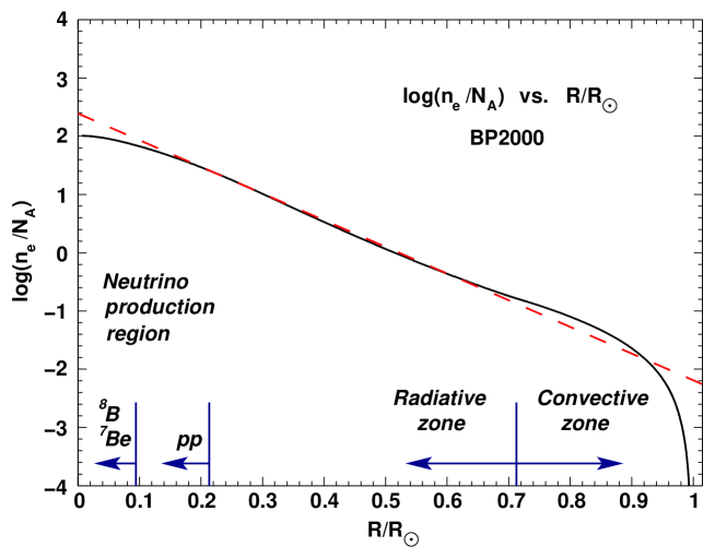
Figure 1: Electron density in the Sun according to the BP2000 [8] solar model. The dashed line shows the best-fit exponential $n_{e}/N_{A}=245\exp(-10.54R/R_{\odot})$.

To get enough conversion, the distance $\delta x$ over which the cancellation persists must be long enough so that a significant fraction of the oscillation cycle can be completed,

$$\Delta\sin 2\theta(\delta x)\mathrel{\mathchoice{\lower 3.0pt\vbox{\halign{$\m@th\displaystyle\hfill#\hfil$\cr>\crcr\sim\crcr}}}{\lower 3.0pt\vbox{\halign{$\m@th\textstyle\hfill#\hfil$\cr>\crcr\sim\crcr}}}{\lower 3.0pt\vbox{\halign{$\m@th\scriptstyle\hfill#\hfil$\cr>\crcr\sim\crcr}}}{\lower 3.0pt\vbox{\halign{$\m@th\scriptscriptstyle\hfill#\hfil$\cr>\crcr\sim\crcr}}}}1.$$ (25)

If one assumes that the profile around the resonance $x=x_{0}$ is approximately linear $A(x)\simeq A(x_{0})+A^{\prime}(x_{0})\delta x$, the width of the resonant region can be written as

$$2\delta x\simeq\frac{2\Delta\sin 2\theta}{A^{\prime}(x_{0})}$$ (26)

and Eq. (25) becomes

$$\frac{2\Delta^{2}\sin^{2}2\theta}{A^{\prime}(x_{0})}\mathrel{\mathchoice{\lower 3.0pt\vbox{\halign{$\m@th\displaystyle\hfill#\hfil$\cr>\crcr\sim\crcr}}}{\lower 3.0pt\vbox{\halign{$\m@th\textstyle\hfill#\hfil$\cr>\crcr\sim\crcr}}}{\lower 3.0pt\vbox{\halign{$\m@th\scriptstyle\hfill#\hfil$\cr>\crcr\sim\crcr}}}{\lower 3.0pt\vbox{\halign{$\m@th\scriptscriptstyle\hfill#\hfil$\cr>\crcr\sim\crcr}}}}1.$$ (35)

Whenever the condition in Eq. (35) is satisfied, one can expect the conversion to be large.

2.2.3 Resonance: level crossing

On closer inspection, it turns out that the conversion is not only large, but can be almost complete. This can most easily understood as the case of adiabatic level crossing, a phenomenon well known in quantum mechanics. If parameters in the Hamiltonian vary slowly enough, the state that was initially created as the eigenstate of the instantaneous Hamiltonian (henceforth, “the matter mass eigenstate”) will follow the changing eigenstate. In the case of solar neutrinos with a small mixing angle and $\Delta\leq 10^{-5}$ eV²/MeV, the flavor eigenstate $\nu_{e}$ in the core almost coincides with the heavy matter mass eigenstate $\nu_{2}$. The heavy mass eigenstate is, in turn, smoothly “connected” to the heavy eigenstate in vacuum which is predominantly composed of $\nu_{\mu}$. The situation is illustrated in Fig. 2.

\psfrag{R/Rsun}{\large$R/R_{\odot}$}\psfrag{nue}{\Large$\sim\nu_{e}$}\psfrag{numu}{\Large$\sim\nu_{\mu}$}\psfrag{0}{\large 0}\psfrag{1}{\large 1}\psfrag{0.2}{\large 0.2}\psfrag{0.4}{\large 0.4}\psfrag{0.6}{\large 0.6}\psfrag{0.8}{\large 0.8}\includegraphics[angle={0},width=338.5863pt]{levelcrossing.eps}

Figure 2: The level crossing in the Sun (small mixing angle).

To see explicitly how the adiabatic evolution works, let us transform the evolution equation, Eq. (1), from the flavor basis $(\nu_{e},\nu_{\mu})$ to the basis of the matter mass eigenstates $(\nu_{1},\nu_{2})$,

$$\phi=V^{\dagger}\psi.$$

Remembering that the rotation matrix

$$V=\left(\begin{array}[]{rr}\cos\theta_{m}&-\sin\theta_{m}\\ \sin\theta_{m}&\cos\theta_{m}\end{array}\right)$$ (38)

is position dependent, we get

$$i\frac{d}{dx}(V^{\dagger}\psi) = HV^{\dagger}\psi,$$

$$i\frac{d\psi}{dx} = VHV^{\dagger}\psi-iV\frac{dV^{\dagger}}{dx}\psi.$$ (39)

Since $VHV^{\dagger}=\mbox{diag}(-\Delta_{m},+\Delta_{m})$ and from Eq. (38)

$$V\frac{dV^{\dagger}}{dx}=\left(\begin{array}[]{rr}0&1\\ -1&0\end{array}\right)\frac{d\theta_{m}}{dx},$$

we obtain the desired evolution equation in the basis of the matter mass eigenstates [10],

$$\frac{d}{dx}\left(\begin{array}[]{c}\psi_{1}\\ \psi_{2}\end{array}\right)=\left(\begin{array}[]{cc}i\Delta_{m}&-d\theta_{m}/dx\\ d\theta_{m}/dx&-i\Delta_{m}\end{array}\right)\left(\begin{array}[]{c}\psi_{1}\\ \psi_{2}\end{array}\right).$$ (46)

This shows that the coupling between the matter mass eigenstates depends on $d\theta_{m}/dx$ and, hence, vanishes when the density change along the neutrino trajectory is very gradual. More precisely, the relevant quantity is the ratio $\Delta_{m}/(d\theta_{m}/dx)$, which at the resonance point equals $2\Delta^{2}\sin^{2}2\theta/A^{\prime}(x_{0})$. Thus the condition for adiabaticity $\Delta_{m}/(d\theta_{m}/dx)\mathrel{\mathchoice{\lower 3.0pt\vbox{\halign{$\m@th\displaystyle\hfill#\hfil$\cr>\crcr\sim\crcr}}}{\lower 3.0pt\vbox{\halign{$\m@th\textstyle\hfill#\hfil$\cr>\crcr\sim\crcr}}}{\lower 3.0pt\vbox{\halign{$\m@th\scriptstyle\hfill#\hfil$\cr>\crcr\sim\crcr}}}{\lower 3.0pt\vbox{\halign{$\m@th\scriptscriptstyle\hfill#\hfil$\cr>\crcr\sim\crcr}}}}1$ is precisely the same as Eq. (35), as should be expected since they both describe the same physics.

2.2.4 Vacuum oscillation solutions

If matter effects are important in the Sun, what about the vacuum oscillation solutions to the solar neutrino problem? Wouldn’t the matter effects also modify the neutrino evolution in that case?

This question can be answered in several steps. First, the vacuum oscillation solutions are characterized by the values of $\Delta m^{2}$ in the range $10^{-11}-10^{-9}$ eV². For $\Delta m^{2}$ in this range, the matter effects are obviously important in the core: the term $A(x)$ completely dominates in Eq. (12), leading to the complete suppression of the oscillations there.

Next, consider what happens in the outer layers on the Sun. If $\Delta/E_{\nu}\sim 10^{-11}$ eV²/MeV, the off-diagonal term in the Hamiltonian is so small that the neutrino does not have any time to oscillate into $\nu_{\mu}$ while still inside the Sun. In other words, the condition (35) in this case is badly violated and the neutrino evolution is extremely nonadiabatic (flavor conserving). In the language of the matter mass eigenstates, this corresponds to the probability of level jumping $P_{c}=\cos^{2}\theta$. One then expects the vacuum oscillations to start up near the surface of the Sun.

Finally, it is worth mentioning that this conclusion does not extend to $\Delta/E_{\nu}\sim 10^{-9}$ eV²/MeV. A careful analysis shows that the neutrino evolution in this range is not extremely nonadiabatic, unlike previously thought, i. e., $P_{c}<\cos^{2}\theta$. For details, see [16].

3 Questions

Above we have described several key features of the neutrino evolution in the Sun. They form the well established physical picture of the MSW mechanism as the “resonant amplification phenomenon”. This picture has become the standard lore over the years. It can be summarized as follows:

• If the evolution is adiabatic, the flavor content of the neutrino state changes as the neutrino traverses the Sun. The flavor conversion occurs around the resonance layer, see Eq. (16).

• To check whether the evolution is adiabatic or not, one should evaluate the adiabaticity condition. This condition becomes the most critical at the resonance, Eq. (35). If the evolution is nonadiabatic, the jumping between the matter mass eigenstates takes place. This jumping also happens mostly in the resonance layer.

This picture is remarkably simple and at the same time very successful in describing the neutrino evolution when the mixing angle is small. It, however, encounters serious difficulties explaining physics in other cases. We shall next pose several questions that expose the limitations of this picture.

3.1 The relevant part of the density profile

In the preceding discussion we assumed that the density profile was linear. It may not be immediately obvious why this assumption is justified. After all, the electron density throughout the Sun, generally speaking, is not linear. As Figure 1 shows, it falls off more or less exponentially in the radiative zone, while deviating from the exponential near the solar edge and also in the core.

More precisely, we assumed that the density can be well approximated by a linear function in some neighborhood $(x_{0}-\delta x,x_{0}+\delta x)$ of the resonance point, where $\delta x=2\Delta\sin 2\theta/A^{\prime}(x_{0})$ is the previously introduced width of the resonance region. Obviously, this works well when $A^{\prime\prime}(x_{0})(\delta x)^{2}/2\ll A^{\prime}(x_{0})(\delta x)$, or

$$\Delta\sin 2\theta\ll(A^{\prime}(x_{0}))^{2}/A^{\prime\prime}(x_{0}).$$

We can see that, when the mixing angle $\theta$ is small, the width of the resonance region is also small, so that the linear approximation for the density should be good. The important point is that all the “interesting” physics, i. e. the flavor conversion or level jumping, happens within this region. The jumping probability in this case can be found using the analytical expression for the linear density profile,

$$(P_{c})_{\rm(lin)}=\exp\left(-\pi\frac{\Delta^{2}\sin^{2}2\theta}{A^{\prime}|_{A=\Delta}}\right).$$ (47)

(Notice that the expression in the exponent is up to a factor just the adiabaticity parameter.) The details of the profile outside this region are not so important, so long as the density there is sufficiently different from resonant.

The question is: what happens when the mixing angle is large? According to Eq (26), the resonance region in that case is wide and so the linear approximation may no longer apply. While the analytical expression for the infinite exponential profile [17, 18],

$$P_{c}=\frac{e^{4\pi r_{0}\Delta\cos^{2}\theta}-1}{e^{4\pi r_{0}\Delta}-1},$$ (48)

is not limited to the case of small $\theta$, it is not clear a priori if it can be applied for solar neutrinos, since there we are not dealing with an infinite exponential. If the “interesting” physics, in the sense defined before, happens on the part of the trajectory which does not lie within the exponential part of the profile, we have no justification to use Eq. (48).

The question is not just academic, but has a direct application for the present-day solar neutrino analysis. Recent solar neutrino fits indicate that the so-called Large Mixing Angle (LMA) solution, characterized by $\Delta m^{2}\sim 10^{-5}-10^{-4}$ eV² and $\tan^{2}\theta\sim 0.1-0.9$, gives a marginally better fit than the small mixing angle (SMA) solution. As the mixing angle approaches $\pi/4$, the resonance defined in Eq. (16) occurs closer and closer to the solar surface. Does this mean we need to know the details of the profile in the convective zone of the Sun to reliably compute the neutrino survival probability for the LMA solution? The resonance amplification picture says “yes”, while the numerical computations say “no”.

3.2 The case of “inverted hierarchy”

The next issue is understanding the evolution in the case $\Delta<0$ (“inverted hierarchy”). This means the heavy mass eigenstate in vacuum is made up predominantly of $\nu_{e}$. Since in this case no resonance occurs, it received comparatively little attention in the literature until recently. At the same time, this case raises several interesting questions that are not easy to answer within the traditional resonance framework described above.

First of all, notice that the mixing angles at the production point in the core and in vacuum are different, just like in the $\Delta>0$ case. This means that if the evolution is adiabatic, the flavor composition of the neutrino state changes as it travels through the Sun. Where does this change occur if there is no resonance?

Next, consider the limit of small $\Delta$. For $\Delta\sim 10^{-11}-10^{-10}$ eV²/MeV one expects vacuum oscillations which are no different then in the $\Delta>0$ case. Namely, the flavor oscillations in the solar core are suppressed and in the region close to the solar surface the off-diagonal terms in the Hamiltonian (12) are too small to allow a significant flavor conversion within the Sun. Hence, viewed in the mass basis, the evolution in this case is extremely nonadiabatic. The jumping between the matter mass eigenstates does occur, even if there is no resonance. How can this be?

4 Matter effects and large mixing angles

4.1 Connecting $\Delta<0$ and $\Delta>0$ parts of the parameter space

The two cases, $\Delta<0$ and $\Delta>0$, the way they were described up to this point, might appear qualitatively very different. Nevertheless, it can be easily demonstrated that they are continuously connected.

To see this, notice that the situations 1) $\Delta<0$, $\theta\leq\pi/4$ and 2) $\Delta>0$, $\theta\geq\pi/4$ are physically the same [19, 20]. This can be easily seen from Eqs. (1) and (6). The case $\theta\rightarrow\pi/2-\theta$ reduces to $\Delta\rightarrow-\Delta$ by redefining the sign of, say, $\phi_{\mu}$. Hence the physical parameter space can be continuously parameterized by keeping the sign of $\Delta$ fixed and varying $\theta$ from 0 to $\pi/2$. This means that there should be a unifying physical description of the MSW effect that continuously incorporates the resonant $(\theta<\pi/4)$ and the nonresonant $(\theta>\pi/4)$ cases.

4.2 The points of maximal violation of adiabaticity and maximal flavor conversion do not coincide with the resonance

Such description is not difficult to construct. The two questions we must be able to answer are:

• In the adiabatic case, what defines the center of the region where the flavor conversion takes place?

• In the nonadiabatic case, what defines the center of the region where the jumping between the mass eigenstates occurs?

Once again, the description we are seeking should be continuous across the maximal mixing ($\theta=\pi/4$) and should reduce to the standard resonance picture in the small $\theta$ limit.

The answers to both questions turn out to be straightforward. First, consider the adiabatic case. In this regime the neutrino state is “glued” to the changing mass eigenstate. Hence, one can define the point a which the mass basis rotates at the maximal rate with respect to the flavor basis to be the point where the flavor composition of the state changes at the fastest rate. In other words, we need the point where $\dot{\theta}_{m}\equiv d\theta_{m}/dx$ is maximal.

\psfrag{psi}{{\large$|\psi_{2}|^{2}$}}\psfrag{r, 10^6 km}{{\large$x$, $\times 10^{6}$ km}}\psfrag{pi/3}{{\large$\theta=\pi/3$}}\psfrag{pi/4}{{\large$\theta=\pi/4$}}\psfrag{pi/6}{{\large$\theta=\pi/6$}}\psfrag{pi/60}{{\large$\theta=\pi/60$}}\psfrag{1}{{\large 1}}\psfrag{1.4}{{\large 1.4}}\psfrag{1.2}{{\large 1.2}}\psfrag{1.0}{{\large 1.0}}\psfrag{0.8}{{\large 0.8}}\psfrag{0.6}{{\large 0.6}}\psfrag{0.4}{{\large 0.4}}\psfrag{0.2}{{\large 0.2}}\includegraphics[angle={0},width=338.5863pt]{transition.eps}

Figure 3: Neutrino state evolution in the case of the infinite exponential density profile for $\Delta m^{2}/E_{\nu}=10^{-9}$ eV²/MeV. The plot shows the probability of finding the neutrino in the heavy matter mass eigenstate $\nu_{2}$ as a function of position $x$, for four different values of the vacuum mixing angle. The points of the maximal violation of adiabaticity, as predicted by Eq. (56), are marked.

To get some understanding of where this point lies, let us find it explicitly for the infinite exponential profile $A(x)\propto\exp(-x/r_{0})$. Using $A^{\prime}(x)=-A(x)/r_{0}$ and

$$\dot{\theta}_{m} = \frac{\sin^{2}2\theta_{m}}{2\Delta\sin 2\theta}\frac{dA}{dx},$$ (49)

$$A = \frac{\Delta\sin(2\theta_{m}-2\theta)}{\sin 2\theta_{m}},$$ (50)

we find that $\dot{\theta}_{m}\propto\sin 2\theta_{m}\sin(2\theta_{m}-2\theta)=(\cos 2\theta-\cos(4\theta_{m}-2\theta))/2$, and so the maximum occurs when

$$\theta_{m}^{\rm max}=\pi/4+\theta/2,$$ (51)

i. e., when $\theta_{m}$ is halfway between its value deep in the core $(\pi/2)$ and its value in vacuum $(\theta)$. The corresponding value of the matter term at this point is

$$A(\theta_{m}^{\rm max})=\Delta.$$ (52)

Notice that conditions in Eqs. (51) and (52) are completely general, valid for all values of the mixing angle. Notice also that they agree with the resonance description

$$A(x_{0})=\Delta\cos 2\theta,$$ (53)

$$\theta_{m}(x_{0})=\pi/4,$$ (54)

in the limit $\theta\ll 1$, as expected. Thus, the resonance amplification interpretation is just a particular limit of this general physical picture.

Now consider the nonadiabatic case. The “level jumping” region will be centered around the point of maximal violation of adiabaticity, which corresponds to the minimum of $\Delta_{m}/\dot{\theta}_{m}$, as discussed in Sect. 2.2.3. Since $\dot{\theta}_{m}\rightarrow\infty$ deep inside the Sun and also in vacuum, the minimum of $\Delta_{m}/\dot{\theta}_{m}$, unlike the resonance, exists for all values of $\theta$.

Once again, let us demonstrate this on the example of the exponential profile. A short calculation shows that the minimum in this case occurs when

$$\cot(2\theta_{m}-2\theta)+2\cot(2\theta_{m})=0,$$ (55)

or

$$A=\Delta\frac{\cos 2\theta+\sqrt{8+\cos^{2}2\theta}}{4}.$$ (56)

Thus, the density at the center of the nonadiabatic part of the neutrino trajectory varies between $A=\Delta$ ($\theta\rightarrow 0$) and $A=\Delta/2$ ($\theta\rightarrow\pi/2$). The resonance description again only works when $\theta\ll 1$. As $\theta\rightarrow\pi/4$, the resonance moves to infinity, while the true point of maximal violation of adiabaticity moves only to the point where $A=\Delta/\sqrt{2}$.

The situation is illustrated in Fig. 3, which shows the probability of finding the neutrino in the heavy mass state $\nu_{2}$ as a function of the distance $x$. The parameters of the exponential were taken from the fit line in Fig. 1 and $\Delta m^{2}/E_{\nu}=10^{-9}$ eV²/MeV. Three large values of the mixing angle ($\theta=\pi/6,\pi/4,\mbox{ and }\pi/3$) and one small value ($\theta=\pi/60$) were chosen. The dashed lines and dots mark the points where adiabaticity is maximally violated, as predicted by Eq. (56). One can see that the partial jumping into the light mass eigenstate in all four cases indeed occurs around the marked points.

\psfrag{tan}{{\large$\tan^{2}\theta$}}\psfrag{dm2}{{\large$\Delta m^{2}/E_{\nu}$, (eV${}^{2}$/MeV)}}\psfrag{0}{{\large$1$}}\psfrag{1}{{\large$10$}}\psfrag{2}{{\large$10^{2}$}}\psfrag{3}{{\large$10^{3}$}}\psfrag{-1}{{\large$10^{-1}$}}\psfrag{-2}{{\large$10^{-2}$}}\psfrag{-3}{{\large$10^{-3}$}}\psfrag{7}{{\large$10^{-7}$}}\psfrag{8}{{\large$10^{-8}$}}\psfrag{9}{{\large$10^{-9}$}}\psfrag{10}{{\large$10^{-10}$}}\psfrag{11}{{\large$10^{-11}$}}\psfrag{Pc=0.9}{{\large$P_{c}=0.9$}}\psfrag{0.7}{{\large$0.7$}}\psfrag{0.5}{{\large$0.5$}}\psfrag{0.3}{{\large$0.3$}}\psfrag{0.1}{{\large$0.1$}}\psfrag{0.01}{{\large$10^{-2}$}}\psfrag{0.001}{{\large$10^{-3}$}}\psfrag{Adiabatic}{{\Large Adiabatic}}\psfrag{Nonadiabatic}{{\Large Nonadiabatic}}\psfrag{Eq1}{{\large Eq. (\ref{eq:oldad0})}}\psfrag{Eq2}{{\large Eq. (\ref{eq:oldad})}}\psfrag{Eq3}{{\large Eq. (\ref{eq:adiabaticity})}}\includegraphics[angle={0},width=435.32419pt]{adiabaticity3.eps}

Figure 4: The boundary between the adiabatic and nonadiabatic regions in the case of the exponential profile, as predicted by Eq. (57), Eq. (58), and Eq. (62). The dashed curves show the contours of constant $P_{c}$. For large angles Eq. (62) provides a better description of the boundary.

4.3 Adiabaticity criterion for large mixing angles

At last, we shall formulate the adiabaticity criterion that is valid for all values of the mixing angle. From the preceding discussion it should be obvious that the criterion of Eq. (35),

$$|\Delta_{m}/\dot{\theta}_{m}|_{\theta_{m}=\pi/4}\gg 1,$$ (57)

should only work in the limit $\theta\ll 1$. At the very least, the quantity $\Delta_{m}/\dot{\theta}_{m}$ should be evaluated at the true point of the maximal violation of adiabaticity. As an estimate, we can approximate it by the point halfway between $\theta$ and $\pi/2$ (see Eq. (51)). We then get

$$|\Delta_{m}/\dot{\theta}_{m}|_{\theta_{m}\sim\pi/4+\theta/2}\gg 1.$$ (58)

This is better, but still not quite right for large $\theta$. The key is to express the information contained in the system of two evolution equations in a single equation. Eq. (1) contains redundant information: while it contains four real functions, the actual number of degrees of freedom is only two, since the normalization of the state is fixed and the overall phase is physically irrelevant. It will be easier to formulate the criterion in question once the two physical degrees of freedom are isolated.

With this in mind, let us write down the evolution equation for the ratio $s\equiv\psi_{1}/\psi_{2}$. From Eq. (46) we obtain the following first order equation:

$$\frac{ds}{dx}=2i\Delta_{m}s-\dot{\theta}_{m}(s^{2}+1),$$ (59)

or

$$\frac{ds}{d\theta_{m}}=2i\frac{\Delta_{m}}{\dot{\theta}_{m}}s-(s^{2}+1).$$ (60)

It is easy to see that the adiabatic limit corresponds to neglecting the terms in parentheses, while the extreme nonadiabatic limit is obtained if one neglects the first term on the right. In the second case the solution is $s=\cot(\theta_{m})$. Thus, the self consistent condition to have the extreme nonadiabatic solution is $2|\Delta_{m}/\dot{\theta}_{m}s|\ll(s^{2}+1)$, with $s=\cot(\theta_{m})$, $\theta_{m}=\pi/4+\theta/2$. In the opposite limit, the evolution is adiabatic. The adiabaticity condition is then

$$|\Delta_{m}/\dot{\theta}_{m}|_{\theta_{m}\sim\pi/4+\theta/2}\gg(\tan(\pi/4+\theta/2)+\cot(\pi/4+\theta/2))/2,$$ (61)

or, upon simplification,

$$\cos\theta|\Delta_{m}/\dot{\theta}_{m}|_{\theta_{m}\sim\pi/4+\theta/2}\gg 1.$$ (62)

Eq. (62) is valid for all values of the mixing angle.

To illustrate this result, let us again consider the case of the infinite exponential profile. Eq. (62) in this case becomes

$$8\Delta r_{0}\sin^{2}\theta\gg 1.$$ (63)

The solid line in Fig. 4 shows the contour of $8\Delta r_{0}\sin^{2}\theta=1$ computed for $r_{0}=R_{\odot}/10.54$ (the fitted value in the BP2000 solar model, see Fig. 1). For comparison, the dash-dotted curves shows the corresponding prediction of Eqs. (57) and (58). The dashed curves are the contours of constant $P_{c}$ computed using Eq. (48). It is clear from the Figure that the description of Eq. (62) is correct not only for small $\theta$, but also for $\theta\mathrel{\mathchoice{\lower 3.0pt\vbox{\halign{$\m@th\displaystyle\hfill#\hfil$\cr>\crcr\sim\crcr}}}{\lower 3.0pt\vbox{\halign{$\m@th\textstyle\hfill#\hfil$\cr>\crcr\sim\crcr}}}{\lower 3.0pt\vbox{\halign{$\m@th\scriptstyle\hfill#\hfil$\cr>\crcr\sim\crcr}}}{\lower 3.0pt\vbox{\halign{$\m@th\scriptscriptstyle\hfill#\hfil$\cr>\crcr\sim\crcr}}}}\pi/4$.

5 Conclusions

We have seen that the neutrino evolution in the Sun can be described as the resonance phenomenon only in the limit $\theta\ll 1$. For large values of $\theta$, including $\theta>\pi/4$, the resonance condition does not correspond to anything physical and one instead should simply be thinking about either adiabatic or nonadiabatic evolution.

Since the physics is continuous across $\theta=\pi/4$, there is no reason to truncate the solar neutrino parameter space at maximal mixing. In fact, the latest solar neutrino fits correctly present their results in the $0\leq\theta\leq\pi/2$ parameter space [21, 22].

Notice, that so long as the neutrino survival probability is computed numerically using the full solar density profile, the results are unaffected by the considerations presented here. The value of the preceding arguments is that they give us a correct physical picture of what is going on when neutrinos travel through the Sun and, for example, explain why in the case of the LMA solution the results are not sensitive to the details of the profile in the convective zone, or why the quasivacuum solutions smoothly extend into the region $\theta>\pi/4$. To paraphrase Richard Feynman, we understand the neutrino evolution only if we can predict what should happen in various circumstances without actually having to solve the evolution equations each time.

Finally, it is worth mentioning an important article by A. Messiah [23] which was brought to the attention of the author after Ref. [9] had been submitted to Physical Review. In the article, Messiah considers the mixing angles continuously from $0$ to $\pi/2$ and determines the location of the point of maximal violation of adiabaticity for all values of $\theta$. Even though his adiabaticity criterion disagrees with the one presented here, it was clearly a very important work that, unfortunately, was almost completely forgotten in the subsequent literature.

References

- [1] L. Wolfenstein, Phys. Rev. D17, 2369 (1978).
- [2] S. P. Mikheev and A. Y. Smirnov, Yad. Fiz. (Sov. J. Nucl. Phys.) 42, 913 (1985).
- [3] S. P. Mikheev and A. Y. Smirnov, Nuovo Cim. 9C, 17 (1986).
- [4] B. T. Cleveland et al., Astrophys. J. 496, 505 (1998).
- [5] W. Hampel et al. [GALLEX Collaboration], Phys. Lett. B447, 127 (1999).
- [6] J. N. Abdurashitov et al. [SAGE Collaboration], Phys. Rev. C60, 055801 (1999), astro-ph/9907113.
- [7] S. Fukuda et al. [SuperKamiokande Collaboration], hep-ex/0103032; S. Fukuda et al. [Super-Kamiokande Collaboration], hep-ex/0103033.
- [8] J. N. Bahcall, M. Pinsonneault and S. Basu, astro-ph/0010346, accepted to Astrophys. J.
- [9] A. Friedland, Phys. Rev. D 64, 013008 (2001) [hep-ph/0010231].
- [10] S. P. Mikheev and A. Y. Smirnov, Sov. Phys. JETP 65, 230 (1987).
- [11] H. A. Bethe, Phys. Rev. Lett. 56, 1305 (1986).
- [12] W. C. Haxton, Phys. Rev. Lett. 57, 1271 (1986).
- [13] S. J. Parke, Phys. Rev. Lett. 57, 1275 (1986).
- [14] T. K. Kuo and J. Pantaleone, Rev. Mod. Phys. 61, 937 (1989).
- [15] E. Lisi, A. Marrone, D. Montanino, A. Palazzo and S. T. Petcov, Phys. Rev. D 63, 093002 (2001) [hep-ph/0011306].
- [16] A. Friedland, Phys. Rev. Lett. 85, 936 (2000), hep-ph/0002063.
- [17] S. T. Petcov, Phys. Lett. B200, 373 (1988).
- [18] S. Toshev, Phys. Lett. B 196, 170 (1987).
- [19] G. L. Fogli, E. Lisi and D. Montanino, Phys. Rev. D 54, 2048 (1996) [hep-ph/9605273].
- [20] A. de Gouvea, A. Friedland, and H. Murayama, Phys. Lett. B490, 125 (2000), hep-ph/0002064.
- [21] J. N. Bahcall, P. I. Krastev and A. Y. Smirnov, JHEP 0105, 015 (2001) [hep-ph/0103179].
- [22] M. C. Gonzalez-Garcia, M. Maltoni and C. Pena-Garay, hep-ph/0105269.
- [23] A. Messiah, In Proceedings of the Sixth Moriond Workshop on Massive Neutrinos in Astrophysics and in Particle Physics, Tignes, France, 1986, pp. 373-389.