Analyses of multiplicity distributions at Tevatron by a two-component stochastic model
— No leading particle effect in E735 Experiment —

Abstract

Comparisons of multiplicity distributions at $\sqrt{s}=1.8$ TeV (E735 Experiment and CDF Collaboration) with our predictions by a two-component stochastic model have been made. This stochastic model is described by the pure-birth and Poisson processes. It is found that there are discrepancies among data at the CERN Sp̄pS collider and those at the Tevatron collider. The latter data by E735 do not contain the leading particle effect described by the Poisson process, providing that the view of the two-component stochastic model is correct. The data by CDF contain small leading particle effect. The reason is probably attributed to the correction made by E735, which is necessary to make the data of the full phase space from the restricted rapidity $|\eta|<3.25$.

1 Introduction

In 1993, we made predictions for multiplicity distributions at the Tevatron collider by a two-component stochastic model including the pure-birth (PB) process and the Poisson process [1]. See also [2]. Those predictions have been based on analyses of $C_{q}=\langle n^{q}\rangle/\langle n\rangle^{q}$ ($q=3\sim 5$) in the energy range $\sqrt{s}=11.5\sim 900$ GeV [3, 4, 5, 6, 7, 8, 9, 10, 11, 12]. The method of an extrapolation has been utilized for the predictions.

On the other hand, recently Alexopoulos et al., the E735 Experiment at the FNAL [13] has reported the multiplicity distributions of the full phase space at 300, 546, 1000 and 1800 GeV. The data corrected by the simulation program are shown as the data of full phase space. Thus it is possible to compare our predictions with the multiplicity distributions at the Tevatron collider. Indeed we are very interested in these comparisons, because we can confirm whether or not the hadronization process is ruled by the two-component stochastic model.

In the next paragraph, the two-component stochastic model is introduced. In the 3rd paragraph, we compare the predictions with observed data by E735 at the Tevatron at $\sqrt{s}=1.8$ TeV. In the 4th one, we consider why there are discrepancies among the predictions and the data by E735 at the Tevatron. In the final one, we present our concluding remarks.

2 Two-component stochastic model

We explain briefly the essentials of the two-component stochastic model used in ref. [1]. It is based on the following two-component branching equation for the two-component probability $P(n_{a},n_{b};t)$:

$$\frac{\partial P(n_{a},n_{b};t)}{\partial t} = \mu\left[P(n_{a}-1,n_{b};t)-P(n_{a},n_{b};t)\right]$$ (1)

$$+\lambda\left[(n_{b}-1)P(n_{a},n_{b}-1;t)-n_{b}P(n_{a},n_{b};t)\right].$$

In eq. (1) the Poisson component (type $a$ particles) and the pure-birth (PB) component (type $b$ particles) do not couple to each other: The former is mainly related to particles in the fragmentation region whereas the latter is related to those in the central region. The two-component probability $P(n_{a},n_{b};t)$ is therefore a product of multiplicity distributions for the Poisson component, $P_{a}(n_{a};t)$ and the corresponding one for the PB component, $P_{b}(n_{b};t)$:

$$P(n_{a},n_{b};t)=P_{a}(n_{a};t)P_{b}(n_{b};t),$$ (2)

and the multiplicity distribution in the final state (i.e., for maximum $t=T$ (the maximum value of an evolution time)) is

$$P(n)=\sum_{n_{a}+n_{b}=n}P(n_{a},n_{b};T),$$ (3)

Figure 1: Illustration of the two-component stochastic model: The dashed line denotes the virtual source $(S)$ which cannot be observed. The particles $a$ are produced by the Poisson process, and $b$ by the PB process.

Here we use the following initial condition [2]:

$$P(n_{a},n_{b};t=0)=\frac{n_{a0}^{n_{a}}}{n_{a}!}e^{-n_{a0}}\frac{n_{b0}^{n_{b}}}{n_{b}!}e^{-n_{b0}},$$ (4)

which leads to

$$P_{a}(n_{a},\langle n_{a}\rangle)=\frac{\langle n_{a}\rangle^{n_{a}}}{n_{a}!}e^{-\langle n_{a}\rangle},$$ (5)

and

$$P_{b}(n_{b},\langle n_{b}\rangle)=\left\{\begin{array}[]{ll}e^{-n_{b0}}&\mbox{ for }n_{b}=0\\ \vskip 2.84544pt\cr\displaystyle{\frac{\langle n_{b}\rangle}{n_{b}}\frac{p^{n_{b}-1}}{(1+p)^{n_{b}+1}}}e^{-n_{b0}}L_{n_{b}-1}^{(1)}\left(-\displaystyle{\frac{n_{b0}}{p}}\right)&\mbox{ for }n_{b}\geq 1,\end{array}\right.$$ (6)

where $p=e^{\lambda T}-1$. Here and after $L^{(k)}_{n}(-x)$ denotes the normalized Laguerre polynomials. The total multiplicity distribution is therefore given by

$$P(n) = \sum_{n_{a}+n_{b}=n}P_{a}(n_{a},\langle n_{a}\rangle)P_{b}(n_{b},\langle n_{b}\rangle)$$ (7)

$$= e^{-(\langle n_{a}\rangle+n_{b0})}\left[\frac{\langle n_{a}\rangle^{n}}{n!}+\sum_{j=1}^{n}\frac{\langle n_{a}\rangle^{n-j}}{(n-j)!}\left(\frac{p}{1+p}\right)^{j}\frac{1}{j}\frac{n_{b0}}{p}L_{j-1}^{(1)}\left(-\displaystyle{\frac{n_{b0}}{p}}\right)\right].$$

The corresponding factorial moments for this $P(n)$ are given by

$$F^{(l)} = \langle n(n-1)\cdots(n-l+1)\rangle$$ (8)

$$= \langle n_{a}\rangle^{l}+\sum_{j=1}^{l}{l\choose j}\langle n_{a}\rangle^{l-j}\Gamma(j)\langle n_{b}\rangle p^{j-1}L_{j-1}^{(1)}\left(-\frac{\langle n_{b}\rangle}{p}\right).$$

The $C_{q}$ moments which we calculate in what follows are easily derived from $F^{(l)}$. We use the same parameters: $\mu T$, $n_{a0}$, $\lambda T$ and $n_{b0}$ [1] which were determined by fits to data for energies $\sqrt{s}=11.5\sim 900$ GeV [3, 4, 5, 6, 7, 8, 9, 10, 11, 12] by choosing minimum chi-squared of sum of $C_{q}\>(q=2\sim 5)$. Finally we have the following expressions:

$$\frac{\langle n_{b}\rangle}{n_{b0}} = \exp(\lambda T)=\exp\left(\lambda\ln\sqrt{s/s_{0}}\right),$$ (9)

$$\langle n_{a}\rangle = \mu T+n_{a0},$$ (10)

with $n_{b0}=4.2$, $\lambda=0.42\pm 0.01$, $\sqrt{s_{0}}=8.60\pm 0.33$ GeV, $\mu=1.22\pm 0.10$ and $n_{a0}=1.50\pm 0.12$.

3 Comparisons of predictions with data at $\sqrt{s}=1.8$ TeV

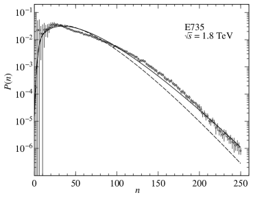
Using eqs. (9) and (10), we can predict $\langle n\rangle$ and $C_{q}=\langle n^{2}\rangle/\langle n\rangle^{2}$ in Table 1 and Fig. 2. Combining the data at $\sqrt{s}=1.8$ TeV in ref. [13] and our predictions, we find that there are discrepancies among our predictions and the data.

Table 1: Prediction for multiplicity by eqs. (9) and (10) and corrected data of the full phase space at the Tevatron

	$\langle n\rangle$	$C_{2}=\langle n^{2}\rangle/\langle n\rangle^{2}$
prediction [1]	$47.88\pm 1.54$	$1.316\pm 0.007$
corrected data at $\sqrt{s}=1.8$ [13]	$45.81\pm 0.77$	$1.45\pm 0.05$

Figure 2: Prediction for multiplicity by eqs. (9) and (10) and data at the Tevatron. The solid line is obtained by $\langle n\rangle=47.88+1.54$ and $C_{2}=1.316+0.007$. The dashed line is obtained by $\langle n\rangle=47.88-1.54$ and $C_{2}=1.316-0.007$.

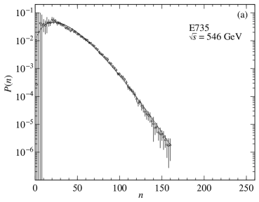
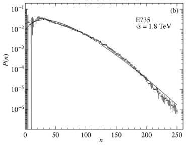
To elucidate the reasons, we adopt other ways. Using eq. (7) with the CERN-MINUIT program, and the multiplicity distributions at the FNAL, the CERN Sp̄pS and the Tevatron, we obtain various results given in Table 2. See Fig. 3.

Table 2: Analyses of data [3, 4, 5, 6, 7, 8, 9, 10, 11, 12, 13] by eqs. (7) $\sim$ (10) with the CERN MINUIT program. $\langle n\rangle=\langle n_{a}\rangle+\langle n_{b}\rangle$ with $\langle n_{b}\rangle=\frac{1}{2}n_{b0}[1+\sqrt{1+2\langle n\rangle^{2}(C_{2}-1-1/\langle n\rangle)/n_{b0}}]$. The data by UA5 [10, 11, 12] are arranged by means of $\sigma_{\tiny\rm NSD}=\sigma_{\tiny\rm ND}+\sigma_{\tiny\rm DD}$, where NSD, ND and DD stand for “non-single diffractive”, “non-diffractive” and “double diffractive”, respectively.

Exps.	$n_{b0}$	$\langle n\rangle$	$C_{2}$	$\langle n_{a}\rangle$	$\chi^{2}/N_{dof}$
FNAL 300 GeV	5.301$\pm$0.423	8.433	1.259$\pm$0.028	0	24.2/11
FNAL 800 GeV	5.370$\pm$0.053	10.16	1.274$\pm$0.004	0	48.1/13
ISR 30.4 GeV	2.711$\pm$0.611	10.58$\pm$0.13	1.186$\pm$0.006	5.259	19.5/14
ISR 44.5 GeV	2.744$\pm$0.541	12.11$\pm$0.11	1.198$\pm$0.007	5.731	5.12/16
ISR 52.6 GeV	4.366$\pm$0.677	12.73$\pm$0.10	1.206$\pm$0.005	3.487	4.73/18
ISR 62.2 GeV	6.540$\pm$1.417	13.67$\pm$0.129	1.194$\pm$0.005	1.212	22.5/17
UA5 200 GeV	3.419$\pm$0.592	21.46$\pm$0.29	1.249$\pm$0.010	7.005	9.58/28
UA5 546 GeV	3.360$\pm$0.180	29.52$\pm$0.18	1.277$\pm$0.004	8.893	53.0/44
UA5 900 GeV	2.703$\pm$0.160	35.93$\pm$0.33	1.292$\pm$0.007	13.08	55.6/51
E735 300 GeV	5.963$\pm$0.018	25.97	1.297$\pm$0.001	0	65.8/57
E735 546 GeV	4.993$\pm$0.020	31.06	1.368$\pm$0.002	0	49.2/77
E735 1000 GeV	4.699$\pm$0.020	38.96	1.400$\pm$0.002	0	112.9/74
E735 1800 GeV	4.565$\pm$0.002	46.36	1.417$\pm$0.000	0	330.6/122

Figure 3: (a) Analyses of data at $\sqrt{s}=546$ GeV by eq. (7) with the CERN MINUIT program. $\chi^{2}/N_{dof}=49.2/77$. (b) Analyses of data at $\sqrt{s}=1.8$ TeV. $\chi^{2}/N_{dof}=330.6/122$.

Table 2 shows that the data at the Tevatron do not contain the multiplicity by the Poisson process in eq. (7), because $\langle n_{a}\rangle=0$. On the other hand, the leading particle effect (finite $\langle n_{a}\rangle$) can be observed in the data by UA5 and in the ISR regions.

4 Differences between data by UA5 and those at Tevatron

To consider the reason of $\langle n_{a}\rangle=0$ at the Tevatron, we analyse the data at $\sqrt{s}=546$ GeV and $\sqrt{s}=1.8$ TeV by CDF Collaboration [14]. What we expect is small $\langle n_{a}\rangle$’s, because of no correction by the simulation program in ref. [14]. Indeed we find that the magnitude of $\langle n_{a}\rangle$ is small, due to the restriction of the pseudo-rapidity cutoff $|\eta|<3.25$. This fact suggests that the data by CDF mainly produced in the central region. (See also [15].)

Table 3: Analyses of data [14] by eqs. (7) $\sim$ (10). Data are read by eye-balls from their Fig. 10.

Exps.	$n_{b0}$	$\langle n\rangle$	$C_{2}$	$\langle n_{a}\rangle$	$\chi^{2}/N_{dof}$
CDF 546 GeV	6.708$\pm$0.348	36.03$\pm$0.21	1.242$\pm$0.004	1.967	201.2/43
CDF 1.8 TeV	4.754$\pm$0.150	45.22$\pm$0.40	1.358$\pm$0.007	2.344	157.0/64

As the next step, we carefully compare the data at $\sqrt{s}=546$ GeV by UA5 and E735. We find that the comparison of the data ($\sqrt{s}=546$ GeV) of UA5 and E735 shows us that error bars of low multiplicities $\delta P(n)\ (n=2,\,4,\,6)$ at the Tevatron are larger than those by UA5. Then we can examine the above observation by making a pseudo-multiplicity at $\sqrt{s}=546$ GeV as follows: The magnitude of error bars $\delta P(n)$ at $n=2,\ 4$ are assumed to be $\delta P(n)\sim P(n)\ (n=2,\ 4)$ in Table 4, to consider our problem. As the same situation is seen in $P(n)$ at $\sqrt{s}=1.8$ TeV in Table 5 , we make two kinds of pseudo-multiplicity distributions and analyse them.

Table 4: $P(n)$ and pseudo-$P(n)$ with $\delta P(n)\sim P(n)$ $(n=2,\ 4)$ at $\sqrt{s}=546$ GeV

	$P(n)$	$P(n)$	pseudo-$P(n)$ with
	$\sqrt{s}=546$ GeV	$\sqrt{s}=546$ GeV	$\delta P(n)\sim P(n)\ (n=2,\ 4)$
	UA5	E735 Experiment	$\sqrt{s}=546$ GeV E735
$n$	(real $P(n)\pm\delta P(n)$)	(real $P(n)\pm\delta P(n)$)	(pseudo-$P(n)\pm\delta P(n)$)
$2$	$0.0027\pm 0.0008$	$2.66\times 10^{-4}\pm 0.0997$	$2.66\times 10^{-4}\pm 2.66\times 10^{-4}$
$4$	$0.0077\pm 0.0013$	$0.0201\pm 0.0799$	$0.0201\pm 0.0201$
$6$	$0.0122\pm 0.0014$	$0.0423\pm 0.0571$	the same as left column
$8$	$0.0195\pm 0.0017$	$0.0364\pm 0.0496$	$\vdots$
$\vdots$	$\vdots$	$\vdots$
$\chi^{2}/N_{dof}$	$53.0/44$	$49.2/77$	$80.3$
$(\langle n_{a}\rangle,\>\langle n_{b}\rangle)$	$(8.89,\>20.63)$	$(0,\>31.06)$	$(8.09,\>24.17)$
$\langle n\rangle$	$29.52\pm 0.18$	$31.06$	$32.26\pm 0.32$
$C_{2}$	$1.277\pm 0.004$	$1.368\pm 0.002$	$1.304\pm 0.007$

Table 5: The same as Table 4 but $\sqrt{s}=1.8$ TeV

	P(n)	1st pseudo-$P(n)$	2nd pseudo-$P(n)$ with
	$\sqrt{s}=1.8$ TeV	$P(2)=P(4)=0$	$\delta P(n)\sim P(n)\ (n=2,\ 4)$
	E735 Experiment	$\sqrt{s}=1.8$ TeV E735	$\sqrt{s}=1.8$ TeV E735
$n$	(real $P(n)\pm\delta P(n)$)	(pseudo-$P(n)\pm\delta P(n)$)	(pseudo-$P(n)\pm\delta P(n)$)
$2$	$1.75\times 10^{-4}\pm 0.1038$	$0$	$1.75\times 10^{-4}\pm 1.75\times 10^{-4}$
$4$	$0.0223\pm 0.0291$	$0$	$0.0223\pm 0.0223$
$6$	$0.0224\pm 0.0327$	the same as left column	the same as left column
$8$	$0.0167\pm 0.0150$	$\vdots$	$\vdots$
$\vdots$	$\vdots$
$\chi^{2}/N_{dof}$	$330.6/122$	$314.8/120$	$432.3/122$
$(\langle n_{a}\rangle,\>\langle n_{b}\rangle)$	$(0,\>46.36)$	$(0,\>46.82)$	$(7.94,\>39.26)$
$\langle n\rangle$	$46.36$	$46.82$	$47.21\pm 0.19$
$C_{2}$	$1.417\pm 0.000$	$1.410\pm 0.000$	$1.372\pm 0.003$

The results of Tables 4 and 5 show that $\langle n_{a}\rangle$ and $C_{2}$ depend on the magnitudes of error bars at $n=$ 2 and 4, as is shown by analysing the pseudo-$P(n)$’s. The low multiplicities with larger error bars are equal to $P(2)=P(4)=0$, as is seen in the first pseudo-$P(n)$ in Table 5. We find that $\langle n_{a}\rangle$ from the second pseudo-$P(n)$ in Table 5 is coincided with the prediction of Table 1. Thus, it can be said that the leading particle effect is relating to low multiplicities and the magnitude of error bars.

5 Concluding remarks

We have compared our predictions [1] for the multiplicity distribution at 1.8 TeV, based on the two-component model, and the data at the Tevatron by E735. It is found that there are discrepancies between them. See Fig. 2 and Table 1.

To elucidate physical reason of the discrepancies, we have analysed the data by means of the two-component model. From this procedure, we have known that the data by UA5 contain the reading particle effect, finite $\langle n_{a}\rangle$. On the other hand, the data by the Tevatron do not contain it .

As the next step, we have resolved the reason why the data by the Tevatron do not contain $\langle n_{a}\rangle$. For this purpose, we analyse the data by CDF [14] and find small $\langle n_{a}\rangle$ at $\sqrt{s}=546$ GeV and 1.8 TeV. See Table 3. Moreover, we compare the data by UA5 and at the Tevatron in Tables 4 and 5 and find that the error bars of low multiplicities, $\delta P(n)$ ($n=2,\ 4,\ 6$) are large. To see how our result depends on large $\delta P(n)$ ($n=2,\ 4,\ 6$), we have made the pseudo-multiplicity distribution, assuming $\delta P(n)\approx P(n)$ at $n=2$ and $4$. From the pseudo-multiplicity distribution, we can estimate the finite leading particle effect at $\sqrt{s}=546$ GeV and 1.8 TeV at the Tevatron. The result of $\langle n_{a}\rangle\approx 8$ from the second pseudo-$P(n)$ in Table 5 is almost the same of our prediction [1]. (See Table 1.)

In conclusion, we have found that the corrected data of full phase space at Tevatron by E735 do not contain the leading particle effect which is observed in the data by UA5. It is difficult to estimate this effect, because of larger error bars at low multiplicities, $P(n)\pm\delta P(n)$ ($n=2,\ 4$) . In other words, the low multiplicities with $\delta P(n)>P(n)$ $(n=2,\ 4)$ are equivalent to $P(n)=0$ $(n=2,\ 4)$. They are playing important roles for determining the leading particle effect which is expected in ref. [1].

Moreover, providing $P(n,\ \delta\eta)$ with the pseudo-rapidity cutoff in a future, we could obtain more useful information for the production mechanism which are illustrated in Fig. 4: The pure-birth (PB) process mainly describes $P(n)$ in the central region. On the other hand, the Poisson process mainly does $P(n)$ in the fragmentation region .

Figure 4: $d\sigma/d\eta$ distribution. The PB and the Poisson processes probably rule the central and fragmentation regions, respectively.

References

• [1] T. Mizoguchi, M. Biyajima and G. Wilk, Phys. Lett. B 301 (1993) 131; see also T. Mizoguchi, T. Aoki, M. Biyajima and N. Suzuki, Prog. Theor. Phys. 88 (1992) 391.
• [2] M. Biyajima et al., Phys. Rev. D 43 (1991) 1541; see also M. Biyajima, T. Kawabe, and N. Suzuki, Phys. Lett. B 189 (1987) 466; B. Durand and I. Sarcevic, Phys. Lett. B 172 (1986) 104; R. C. Hwa and C. S. Lam, Phys. Lett. B 173 (1986) 346.
• [3] V. V. Ammosov et al., Phys. Lett. B 42 (1972) 519.
• [4] W. M. Morse et al., Phys. Rev. D 15 (1977) 66.
• [5] S. Barish et al., Phys. Rev. D 9 (1974) 2689.
• [6] A. Firestone et al., Phys. Rev. D 10 (1974) 2080.
• [7] C. Bromberg et al., Phys. Rev. Lett. 31 (1973) 1563.
• [8] J. Whitmore, Phys. Rep. 10 (1974) 273.
• [9] A. Breakstone et al., Phys. Rev. D 30 (1984) 528.
• [10] UA5 Collaboration, G. J. Alner et al., Phys. Lett. B 138 (1984) 304; B 160 (1985) 199; B 167 (1986) 476.
• [11] UA5 Collaboration, B. J Alner et al., Phys. Rep. 154 (1987) 247.
• [12] UA5 Collaboration, R. E. Ansorge et al., Z. Phys. C 43 (1989) 357.
• [13] Tevatron Experiment E735, T. Alexopoulos et al., Phys. Lett. B 435 (1998) 453; see also S. G. Matinian and W.D. Walker, Phys. Rev. D 59 (1999) 034022.
• [14] CDF Collaboration, F. Abe et al., Phys. Rev. D 50 (1994) 5550.
• [15] V. D. Rusov et al., Phys. Lett. B 504 (2001) 213.
• [16] Yu. L. Dokshitzer, Phys. Lett. B 305 (1993) 295.
• [17] S. Hegyi, “KNO scaling 30 years later”, hep-ph/0011301 (2000).
• [18] M. Biyajima, Phys. Lett. B 139 (1984) 93.
• [19] F. Takagi and T. Tsukamoto, Phys. Rev. D 38 (1988) 2288.
• [20] A. Ohsawa, Prog. Theor. Phys. 92 (1994) 1005.