FERMILAB-Pub-01/077-T

FTUV-01-05-29

IFIC-01-28

Constraining models with vector-like fermions

from FCNC in $K$ and $B$ physics

G. Barenboim

Theory Division, CERN, CH-1211 Geneva 23, Switzerland and

FERMILAB Th. Group, MS 106 P.O.Box 500, Batavia IL 60510, USA

F.J. Botella and O. Vives

Departament de Física Teòrica and IFIC

Universitat de València-CSIC, E-46100, Burjassot, Spain

In this work, we update the constraints on tree level FCNC couplings in the framework of a theory with $n$ isosinglet vector-like down quarks. In this context, we emphasize the sensitivity of the $B\to J/\psi K_{S}$ $CP$ asymmetry to the presence of new vector-like down quarks. This $CP$ asymmetry, together with the rare decays $B\to X_{s,d}l\bar{l}$ and $K\to\pi\nu\bar{\nu}$ are the best options to further constrain the FCNC tree level couplings or even to point out, in the near future, the possible presence of vector-like quarks in the low energy spectrum, as suggested by GUT theories or models of large extra dimensions at the TeV scale.

1 Introduction

The study of flavor changing neutral currents (FCNC) in particle physics phenomenology has played a key role in the advance of high energy physics in the past decades. Already in the early seventies the non-observation of FCNC was used to predict the existence of the charm quark through the GIM mechanism [1] well before its direct experimental discovery. Subsequently, a precise prediction of its mass was made from FCNC kaon processes [2]. Later on, the discovery of the bottom quark and the measure of the $B$–$\bar{B}$ mass difference indicated the presence of a heavy top quark. Due to this GIM mechanism, FCNC in the SM arise only at higher loop level and are suppressed by powers of light quark masses and small mixing angles. This strong suppression make FCNC phenomena a privileged ground to search for signs of new physics beyond the SM. In many extensions of the SM there is no analog of the GIM mechanism to protect FCNC processes and hence potentially large new physics contributions can be expected. For instance, a minimal supersymmetric extension of the SM with generic soft breaking terms gives rise to dangerously large contributions to FCNC and $CP$ violating observables through loop contributions with the supersymmetric particles running in the loop [3]. Even more challenging (or perhaps more dangerous) than these loop induced FCNCs is the inclusion of tree level FCNC couplings.

Indeed, the presence of tree level FCNC is phenomenologically, a very interesting possibility. A minimal extension of the SM with the only addition of an extra isosinglet down quark in a vector like representation of the SM gauge group induces FCNC couplings in the $Z$ and neutral Higgs boson couplings. Some, more realistic models, include at least one vector-like quark per generation. These models naturally arise, for instance, as the low-energy limit of an $E_{6}$ grand unified theory [4]. Moreover, vector-like quarks can appear in models of large extra dimensions. The existence of extra spatial dimensions of the TeV size implies the existence of towers of Kaluza Klein modes for the particles that propagate in the new (extra) dimensions. Therefore, if some SM fermion propagates in the extra dimensions, for each of these chiral quarks and leptons there is a tower of vector-like fermions whose separation is of order $1/R$, being $R$ the radius of the extra dimensions [5, 6]. From a more phenomenological point of view, models with isosinglet quarks provide the simplest self-consistent framework to study deviations of $3\times 3$ unitarity of the CKM matrix as well as flavor changing neutral currents at tree level. Of course, these FCNC couplings are severely restricted by the low energy results on the different FCNC processes. Nevertheless, it is well known that even fulfilling these strong constraints these couplings can have large effects on $B$ factory experiments on $CP$ violation [8, 10, 11]. In a recent paper [11], we showed that the possible mismatch between the SM expectations and the measured value for the $CP$ asymmetry in the $B\to J/\psi K_{s}$ decay can be easily explained in a model with an additional vector like down quark. In this paper, we complete the previous analysis and generalize it to the case where a tower of vector-like down quarks (VLdQ) is present. In first place, we update the strong low-energy constraints on the tree-level FCNC couplings and then we concentrate on the $CP$ violation observables in the $B$ factories as the most efficient observables to find or at least constrain these tree level FCNC couplings. Finally, we compare the simplest case with a single VLdQ with models with several vector-like down quarks.

2 FCNC in the presence of isosinglet quarks

As explained in the introduction, vector-like fermions appear in different extensions of the SM, as for instance $E_{6}$ GUT models or, remarkably enough, theories with large extra dimensions on the TeV scale. All these models have several new vector like fermions that mix with the SM fermions and can have important effects on the low energy FCNC phenomenology. In this paper, we will study FCNC processes with external down quarks, and so we will be mainly interested in models with isosinglet vector-like down quarks (VLdQ). Note that the presence of extra vector-like down (up) quarks generates FCNC in the down (up) couplings to the $Z$ and $H$. In view of these new possibilities of having VLdQs in the low energy spectrum, and especially, to reach a rough understanding of FCNC effects in models with large extra dimensions [5, 6], we present our bounds in a general framework with $n$ additional VLdQs. A general analysis with both up and down isosinglets and isodoublets will be presented elsewhere [7].

From the low energy point of view, the model we analyze here has been thoroughly described in Ref. [8, 9]. Its main feature is that the additional VLdQs mix with the three ordinary quarks and consequently the mass matrix in the down sector is now $(3+n)\times(3+n)$. This matrix is diagonalized by two $(3+n)\times(3+n)$ mixing matrices and only the left-handed rotation is observable giving rise to the CKM matrix. As we have already announced in the introduction, the fingerprint of this model is that it allows tree level FCNC in the $Z$ and $H$ vertices. To see how these FCNC couplings appear, we can work in the basis where the up quark mass matrix is diagonal. Here the down quark mass matrix is diagonalized by a $(3+n)\times(3+n)$ unitary matrix, $V_{\alpha\beta}$. In this model charged current couplings are unchanged except that $V_{CKM}$ is now the $3\times(3+n)$ upper submatrix of $V$, and at low energies a non-unitary $3\times 3$ mixing matrix appears at tree level. However, the mixing of doublet and singlet weak eigenstates modifies the neutral current couplings that in terms of flavor eigenstates will be $V^{\dagger}\cdot\mbox{Diag.}(1,1,1,0)\cdot V\neq\mbox{I}_{4\times 4}$. So, neutral current interactions are given by,

$${\cal L}_{Z}=\frac{\displaystyle{g}}{\displaystyle{2\cos\theta_{W}}}\left[\bar{u}_{Li}\ \gamma^{\mu}\ u_{Li}\ -\ \bar{d}_{L\alpha}\ U_{\alpha\beta}\ \gamma^{\mu}\ d_{L\beta}\ -\right.$$

$$\left.\ 2\ \sin^{2}\theta_{W}\ J^{\mu}_{em}\right]\ Z_{\mu},$$

$${\cal L}_{H}=\frac{\displaystyle{g}}{\displaystyle{2M_{W}}}\left[\bar{u}_{Li}\ m_{i}^{u}u_{Li}\ -\ \bar{d}_{L\alpha}\ U_{\alpha\beta}\ m_{\beta}^{d}\ d_{L\beta}\right]$$

$$U_{\alpha\beta}=\sum_{i=1}^{3}V_{i\alpha}^{*}V_{i\beta},$$ (1)

where $U_{ds}$, $U_{bs}$ or $U_{bd}\neq 0$ would signal new physics and the presence of FCNC at tree level.

In the following, we analyze the effects of these new couplings in FCNC processes and we update the phenomenological bounds on them. More specifically, in processes changing flavor in one unit, $\Delta F=1$, that in the SM go through electroweak penguin diagrams of order $G_{F}\,\alpha\,V_{ti}^{*}V_{tj}$, we simply consider the dominant tree level FCNC contributions, order $G_{F}U_{ij}$. Similarly in $\Delta F=2$ processes mediated by boxes in the SM of order $G_{F}\,\alpha\,(V_{ti}^{*}V_{tj})^{2}$ we include two different additional contributions, a pure tree level diagram with two FCNC vertices, order $G_{F}U_{ij}^{2}$ and a mixed SM vertex contribution with a tree level vertex, roughly order $G_{F}\,\alpha\,V_{ti}^{*}V_{tj}\,U_{ij}$ [12]. Other new physics contributions in this framework will always be suppressed by additional loop factors or higher powers of the FCNC couplings with respect to the contributions considered here[13]. Therefore the effective low energy theory we consider is then identical to the SM with a non-unitary CKM matrix and the presence of tree level FCNC as shown in Eq. (1).

3 Experimental constraints on the extended mixing matrix

As we have seen in the previous section, all the new physics effects in our model are encoded in the extended mixing matrix that gives rise to tree level FCNC in the $Z$ and $H$ vertices. The minimal extension from the SM would consist in the addition of a single vector-like down quark. In this situation the mixing matrix can be parametrized as [14],

$$V=R_{34}\left(\theta_{34},0\right)R_{24}\left(\theta_{24},\phi_{3}\right)R_{14}\left(\theta_{14},\phi_{2}\right)V_{CKM}^{SM}\left(\theta_{12},\theta_{13},\theta_{23},\phi_{1}\right),$$ (2)

where $V_{CKM}^{SM}\left(\theta_{12},\theta_{13},\theta_{23},\phi_{1}\right)$ is $4\times 4$ block diagonal matrix composed of the standard CKM [15, 16] and a $1\times 1$ identity in the $(4,4)$ element, and $R_{ij}\left(\theta_{ij},\phi_{k}\right)$ is a complex rotation between the $i$ and $j$ “families”. Note that, in the limit of small new angles, we follow the usual phase conventions. In fact, this $4\times 4$ mixing matrix can represent a good approximation to more complete models with several vector-like generations if the mixings are hierarchical, similarly to the standard CKM matrix.

On the other hand, given that the deviations from unitarity of the CKM mixing matrix are experimentally known to be small, it is possible to use an approximate parametrization of the mixing matrix valid for an arbitrary number of vector-like quarks [9]. This is an extension of the usual Wolfenstein parametrization of the CKM [17] in terms of,

$$V_{us}=\lambda\ \ \ \ \ U_{dd}=\sum_{i=u,c,t}|V_{id}|^{2}=1-D^{2}_{d}\ \ U_{sd}=\sum_{i=u,c,t}V_{is}^{*}V_{id}\ \$$

$$V_{cb}=A\lambda^{2}\ \ \ \ U_{ss}=\sum_{i=u,c,t}|V_{is}|^{2}=1-D^{2}_{s}\ \ U_{bs}=\sum_{i=u,c,t}V_{ib}^{*}V_{is}\ \$$

$$V_{ub}=A\mu\lambda^{3}e^{i\phi}\ \ U_{bb}=\sum_{i=u,c,t}|V_{ib}|^{2}=1-D^{2}_{b}\ \ U_{bd}=\sum_{i=u,c,t}V_{ib}^{*}V_{id}\ \$$ (3)

with $(U_{sd},U_{bd},U_{bs})$ general complex numbers and $D^{2}_{j}=\sum_{i=4}^{n+4}|V_{ij}|^{2}$ positive real numbers. It is possible to obtain the remaining elements of the $3\times 3$ submatrix corresponding to the SM mixing matrix as a function of ($\lambda$, $A$, $\mu$, $\phi$, $D^{2}_{d}$, $D^{2}_{s}$, $D^{2}_{b}$, $U_{sd}$, $U_{bd}$, $U_{bs}$). In fact, taking into account that ($D^{2}_{d}$, $D^{2}_{s}$, $D^{2}_{b}$) can be at most of order $\lambda^{3}$ and ($U_{sd}$, $U_{bd}$, $U_{bs}$) are experimentally constrained to be $\leq{\cal O}(\lambda^{4})$, we can keep quadratic or linear terms in ($D^{2}_{d}$, $D^{2}_{s}$, $D^{2}_{b}$) and ($U_{sd}$, $U_{bd}$, $U_{bs}$) respectively and we obtain to ${\cal O}(\lambda^{6})$,

$$V_{ud} = 1-\frac{\displaystyle{\lambda^{2}}}{\displaystyle{2}}-\frac{\displaystyle{\lambda^{4}}}{\displaystyle{8}}-\frac{\displaystyle{1+8A^{2}\mu^{2}}}{\displaystyle{16}}\lambda^{6}-\frac{\displaystyle{D^{2}_{d}}}{\displaystyle{2}}+\frac{\displaystyle{D^{2}_{d}-2D^{2}_{s}}}{\displaystyle{4}}\lambda^{2}-$$

$$\frac{\displaystyle{D_{d}^{4}}}{\displaystyle{8}}+\lambda\mbox{Re}\{U_{sd}\}+{\cal O}(\lambda^{7})$$

$$V_{cs} = 1-\frac{\displaystyle{\lambda^{2}}}{\displaystyle{2}}-\frac{\displaystyle{1+4A^{2}}}{\displaystyle{8}}\lambda^{4}+\frac{\displaystyle{1-4A^{2}+16A^{2}\mu\cos\phi}}{\displaystyle{16}}\lambda^{6}-$$

$$\frac{\displaystyle{D^{2}_{s}}}{\displaystyle{2}}-\frac{\displaystyle{D^{2}_{s}}}{\displaystyle{4}}\lambda^{2}+A\lambda^{2}\mbox{Re}\{U_{bs}\}-\frac{\displaystyle{D_{s}^{4}}}{\displaystyle{8}}+{\cal O}(\lambda^{7})$$

$$V_{tb} = 1-\frac{\displaystyle{A^{2}}}{\displaystyle{2}}\lambda^{4}-\frac{\displaystyle{A^{2}\mu^{2}}}{\displaystyle{2}}\lambda^{6}-\frac{\displaystyle{D^{2}_{b}}}{\displaystyle{2}}-\frac{\displaystyle{D_{s}^{4}}}{\displaystyle{8}}+{\cal O}(\lambda^{7})$$

$$V_{cd} = -\lambda+\left(\frac{\displaystyle{A^{2}}}{\displaystyle{2}}-A^{2}\mu e^{-i\phi}\right)\lambda^{5}+\frac{\displaystyle{D^{2}_{d}-D^{2}_{s}}}{\displaystyle{2}}\lambda+U_{sd}+$$

$$\left(U_{bd}A-\frac{\displaystyle{U_{sd}^{*}}}{\displaystyle{2}}\right)\lambda^{2}+{\cal O}(\lambda^{7})$$

$$V_{td} = A(1-\mu e^{-i\phi})\lambda^{3}+\frac{\displaystyle{A}}{\displaystyle{2}}\mu e^{-i\phi}\lambda^{5}+\frac{\displaystyle{A}}{\displaystyle{2}}D^{2}_{s}\lambda^{3}+U_{bd}+$$

$$\frac{\displaystyle{A}}{\displaystyle{2}}\left(D^{2}_{b}-D^{2}_{d}\right)\left(1-\mu e^{-i\phi}\right)\lambda^{3}-A\lambda^{2}U_{sd}+{\cal O}(\lambda^{7})$$

$$V_{ts} = -A\lambda^{2}+\left(\frac{\displaystyle{A}}{\displaystyle{2}}-A\mu e^{-i\phi}\right)\lambda^{4}+U_{bs}+\frac{\displaystyle{A}}{\displaystyle{2}}\left(D^{2}_{s}-D^{2}_{b}\right)\lambda^{2}+$$ (4)

$$\frac{\displaystyle{A}}{\displaystyle{8}}\lambda^{6}+{\cal O}(\lambda^{7})$$

This is a completely general parametrization of the $3\times 3$ submatrix of a complete $(3+n)\times(3+n)$ unitary matrix. Hence, it includes also the simplest case of a single vector-like quark. In this last case, there are several relations among the 13 parameters of this general matrix and only the nine independent parameters of a unitary $4\times 4$ mixing matrix remain. In fact we have,

$$D_{d}^{2}=|V_{4d}|^{2},\ \ \ \ D_{s}^{2}=|V_{4s}|^{2},\ \ \ \ D_{b}^{2}=|V_{4b}|^{2},$$

$$U_{sd}=-V_{4s}^{*}V_{4d},\ \ \ \ U_{bs}=-V_{4b}^{*}V_{4s},\ \ \ \ U_{bd}=-V_{4b}^{*}V_{4d}.$$ (5)

Hence, we have 4 relations among the parameters in Eq. (3),

$$|U_{sd}|^{2}=D_{s}^{2}D_{d}^{2}\ \ \ \ |U_{bs}|^{2}=D_{b}^{2}D_{s}^{2}$$

$$|U_{bd}|^{2}=D_{b}^{2}D_{d}^{2}\ \ \ \ \ \ \ \ \ \ \ \ \ \ U_{sd}U_{bs}U_{bd}^{*}=D_{b}^{2}D_{s}^{2}D_{d}^{2}.$$ (6)

In the general case these equalities are replaced by inequalities,

$$|U_{sd}|^{2}\leq D_{s}^{2}D_{d}^{2}\ \ \ \ |U_{bs}|^{2}\leq D_{b}^{2}D_{s}^{2}$$

$$|U_{bd}|^{2}\leq D_{b}^{2}D_{d}^{2}\ \ \ \$$ (7)

Naturally, the elements of the extended mixing matrix corresponding to CKM elements are experimentally measured in low energy experiments. Some of these measurements are obtained from tree-level processes, therefore not affected by new physics to a high degree of approximation. Hence they constrain directly the corresponding elements of our extended mixing matrix. Specifically, we have [16, 18], at $95\%$ C.L.,

• $0.2150<|V_{us}|=\lambda<0.2242$,

• $0.0364<|V_{cb}|=A\lambda^{2}<0.0440$,

• $0.074<|V_{ub}/V_{cb}|=\mu\lambda<0.106$,

• $0.9719<|V_{ud}|<0.9751$,

• $0.192<|V_{cd}|<0.256$,

• $0.948<|V_{cs}|<1.0$.

These constraints restrict the different parameters in Eq. (3), and so from the bounds on $|V_{ud}|$ and $|V_{cs}|$, we obtain $D_{d}^{2}\leq 5.5\times 10^{-3}$ and $D_{s}^{2}\leq 5.6\times 10^{-2}$ respectively. Another constraint [8, 9, 19] comes from the $SU(2)_{L}$ coupling of the $Z^{0}$ to $b\overline{b}$. In the SM, this coupling is $(V_{CKM}^{\dagger}\cdot V_{CKM})_{bb}=1$, but in this model it is modified to $U_{bb}$; hence, we have [19] $D_{b}^{2}\leq 9\times 10^{-3}$.

Notice that, in the general case, the $D_{i}^{2}$ parameters are completely independent from the FCNC couplings $U_{\alpha\beta}$. However, in a more definite model, as for instance the single vector-like quark model, due to the unitarity of the $4\times 4$ matrix, these constraints have a strong impact on all other elements of the extended mixing matrix and consequently also on the tree level FCNC couplings, as shown in Eq. (3). In any case, even with these restrictions, the FCNC couplings can have large effects on rare processes, where the SM contributes at the 1 loop level and new physics is allowed to compete on equal footing. In fact, most of the experimental results are well accommodated within a pure 3 generations SM and hence these measurements provide additional constraints on the FCNC couplings. In other observables, like $B^{0}$ $CP$ asymmetries or $B$ rare decays, the experimental results may still differ from the SM prediction once the experimental accuracy is increased in the near future. Therefore, we analyze these observables from a slightly different point of view, and in the last section we show what are the possible deviations from the SM consistent with the constraints discussed here.

In the first place we analyze the constraints associated with kaon physics and then the constraints we get from the B system.

3.1 Kaon physics constraints

Rare kaon decays and $CP$ violating observables in the kaon sector can receive important contributions from the FCNC coupling $U_{sd}$. In fact, this new coupling is constrained mainly by the decay $(K_{L}\rightarrow\mu^{+}\mu^{-})_{SD}$ and the experimental value of $\varepsilon^{\prime}/\varepsilon$. Other observables constraining this coupling are $K^{+}\to\pi^{+}\nu\bar{\nu}$ and $\varepsilon_{K}$ [20].

The decay $K_{L}\rightarrow\mu^{+}\mu^{-}$ is $CP$ conserving and in addition to its short distance part, given by $Z$ penguins and box diagrams, receives important contributions from the two photon intermediate state which are difficult to calculate reliably. Unfortunately, the separation of the short-distance part (similar to $K^{+}\rightarrow\pi^{+}\nu\bar{\nu}$, free of hadronic uncertainties) from the long-distance piece in the measured rate is rather difficult. Therefore, the full branching ratio is generally written as a sum of a dispersive and absorptive contributions, of which the latter can be calculated using the data for $K_{L}\rightarrow\gamma\gamma$. The dispersive contribution can be decomposed as a long distance and a short distance part. Following [20, 21], we can write down,

$$Br\left(K_{L}\rightarrow\mu\overline{\mu}\right)_{SD}=6.32\times 10^{-3}\ \left[C_{U2Z}\ \mbox{Re}\left(U_{sd}\right)\right.$$

$$\left.+\ \bar{\Delta}_{c}+Y_{0}\left(x_{t}\right)\ \mbox{Re}\left(\lambda_{t}^{sd}\right)\right]^{2}\ \leq\ 2.8\times 10^{-9},$$ (8)

where $C_{U2Z}=-(\sqrt{2}G_{F}M_{W}^{2}/\pi^{2})^{-1}\simeq-92.7$, $\lambda_{i}^{ab}=V_{ia}^{\ast}V_{ib}$, $\bar{\Delta}_{c}=-6.54\times 10^{-5}$ is the charm quark contribution and $Y_{0}$ is the Inami-Lim [22] function as defined in [23]. Experimentally, we must require this branching ratio to be $BR(K_{L}\rightarrow\mu^{+}\mu^{-})_{SD}\leq 2.8\times 10^{-9}$ [21].

A second observable constraining $U_{sd}$ is $\varepsilon^{\prime}/\varepsilon$. Within the SM there is a cancellation between QCD and electroweak penguin contributions (dominated by $Z$ penguins) which suppresses this ratio. When new physics enters into the game and if, as it is expected on general grounds, it does not affect considerably the QCD contributions but does so with the $Z$ penguins, the abovementioned cancellation does not take place and significant deviations from the SM results (or strong bounds on the new parameters) can be expected. We now decompose $\varepsilon^{\prime}/\varepsilon$ as follows,

$$\frac{\displaystyle{\varepsilon^{\prime}}}{\displaystyle{\varepsilon}}=\ \beta_{U}\ C_{U2Z}\ \mbox{Im}\left(U_{sd}\right)\ +\ \beta_{t}\ \mbox{Im}\left(\lambda_{t}^{sd}\right)$$

$$\beta_{U}\ =\ [1.2\ -\ R_{s}\ r_{Z}\ B_{8}^{(3/2)}]$$

$$\beta_{t}\ =\ \beta_{U}\cdot C_{0}\ -\ 2.3\ +\ R_{s}\ [1.1\ r_{Z}\ B_{6}^{(1/2)}\ +\$$

$$(1.0\ +\ 0.12\ r_{Z})\ B_{8}^{(3/2)}].$$ (9)

where the first term comes from the $Z$ piece and the other one contains all the remaining ones [20]. It is worth noting that unlike previous observables, here the theoretical errors overwhelm the experimental precision. The main sources of uncertainties lie in the parameters, $B_{6}^{(1/2)}$ and $B_{8}^{(3/2)}$. The importance of these uncertainties is somehow increased because of the cancellation we have mentioned.

Here, we take $R_{s}=1.5\pm 0.5$, $r_{Z}=7.5\pm 1$ and $B_{8}^{(3/2)}=0.8\pm 0.2$ [20]. The value of $B_{6}^{(1/2)}$ has caused some controversy in the literature because of the different values obtained in different schemes. We take two different values in order to illustrate the situation where new physics in the $s$–$d$ sector is needed or not needed to reproduce the experimental value of $\varepsilon^{\prime}/\varepsilon$. For set I, we use $B_{6}^{(1/2)}=1.0\pm 0.2$ with the other parameters as given above, as in Refs. [20, 24, 25] which comes from large $N_{c}$ calculations [26] and lattice analysis, and this tends to favor the presence of new physics in $U_{ds}$. In set II, we use $B_{6}^{(1/2)}=1.3\pm 0.5$ in order to incorporate the predictions of Refs. [27, 28], where inclusion of the correction from final-state interactions in a chiral perturbation theory analysis tends to favor the SM range. Still, there are other schemes where different values for $B_{6}^{(1/2)}$ and $B_{8}^{(3/2)}$ are obtained [29, 30, 31]. In fact, we have explicitly checked that with the values in [29], $B_{6}^{(1/2)}=2.5\pm 0.4$ and $B_{8}^{(3/2)}=1.35\pm 0.20$, the constraints on the FCNC couplings $U_{\alpha\beta}$ are still consistent with the results presented below.

Numerically, we have for the central values

$$\frac{\displaystyle{\varepsilon^{\prime}}}{\displaystyle{\varepsilon}}=\ -7.8\ C_{U2Z}\ \mbox{Im}\left(U_{sd}\right)\ +\ \left\{\begin{array}[]{l}6.2\\ 9.9\end{array}\right.\ \mbox{Im}\left(\lambda_{t}^{sd}\right)$$ (12)

with the parameters in set I and set II respectively and we calculate its errors with a Gaussian method. This observable has to reproduce the experimentally obtained value of $(\varepsilon^{\prime}/\varepsilon)^{exp}=(2.12\pm 0.46)\times 10^{-3}$.

A theoretically cleaner constraint [32], although less restrictive than the previous two constraints is provided by BR($K^{+}\rightarrow\pi^{+}\nu\bar{\nu}$),

$${\rm BR}(K^{+}\rightarrow\pi^{+}\nu\bar{\nu}) = 1.55\cdot 10^{-4}\Biggl{[}\biggl{(}C_{U2Z}Im\{U_{sd}\}+X_{0}(x_{t})\cdot Im\lambda_{t}^{sd}\biggr{)}^{2}$$

$$+\biggl{(}C_{U2Z}Re\{U_{sd}\}-2.11\cdot 10^{-4}+X_{0}(x_{t})Re\lambda_{t}^{sd}\biggr{)}^{2}\Biggr{]}\,,$$

with $X_{0}(x_{t})=C_{0}(x_{t})-4B_{0}(x_{t})$ a gauge invariant loop function combination of boxes and vertices [22, 23]. This decay has already been measured in the experiment E787 at BNL [33], however, so far, a single event has been found and this is not enough to provide a definite value for the branching ratio. Hence we take here only the upper limit at $95\%$ C.L. $\mbox{BR}(K^{+}\rightarrow\pi^{+}\nu\bar{\nu})\leq 8.3\times 10^{-10}$ .

Finally, we include also $\varepsilon_{K}$, whose leading-order expression is [23, 12]:

$$\varepsilon_{K}=\frac{\displaystyle{e^{i\pi/4}G_{F}B_{K}F_{K}^{2}m_{K}}}{\displaystyle{6\Delta m_{K}}}\ \mbox{Im}\left\{-\eta_{tt}\left(U_{sd}\right)^{2}+\frac{\displaystyle{\alpha}}{\displaystyle{4\pi\sin^{2}\theta_{W}}}\right.$$

$$\left.\left[8\sum\limits_{i=c}^{t}\ \eta_{ti}Y_{0}\left(x_{i}\right)\ \lambda_{i}^{sd}U_{sd}\ -\sum\limits_{i,j=c}^{t}\ \eta_{ij}S_{0}(x_{i},x_{j})\ \lambda_{i}^{sd}\lambda_{j}^{sd}\right]\right\}$$ (14)

where $S_{0}$ is another Inami-Lim function [23] and the QCD correction factors (which take into account short distance QCD effects) are given as follows,

$$\eta_{cc}=1.38\pm 0,20,\;\;\;\;\;\;\eta_{tt}=0.57\pm 0.01\;\;\;\;\;\;\eta_{tc}=0.47\pm 0.04$$ (15)

Here, contrary to Ref. [20], the coefficient $Y_{0}\left(x\right)$ of the linear term in $U_{ds}$ is characteristic of the present model, therefore, in principle, the irrelevance of $\varepsilon_{K}$ to constraint $U_{ds}$ is not fully guaranteed.

At this point, it is important to emphasize that Eqs. (8), (9), (3.1) and (14) are completely valid in the general model with $n$ additional VLdQs.

In Fig. 1 we present the effects of the different constraints in the $U_{sd}$ coupling. As we can see in this figure, the most efficient constraints are provided by $K_{L}\rightarrow\mu^{+}\mu^{-}$, that constrains $\mbox{Re}(U_{sd})$, and $\varepsilon^{\prime}/\varepsilon$, that bounds $\mbox{Im}(U_{sd})$ to the rectangular box in the center. However, these constraints will be difficult to improve due to the large hadronic uncertainties. Similarly, the constraints from $\varepsilon_{K}$ are very precise on the experimental side and the precision of this limit on $U_{sd}$ is determined by the hadronic parameter $B_{K}=0.85\pm 0.15$ [23, 25].

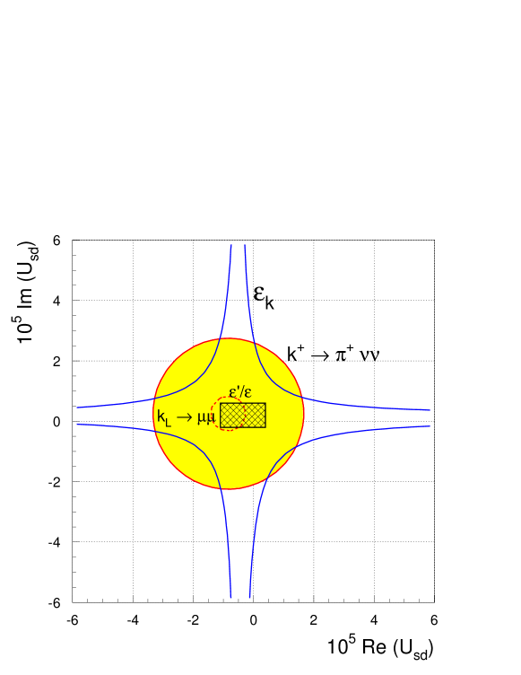
Figure 1: Effect of the constraints from $\varepsilon_{K}$, $K^{+}\rightarrow\pi^{+}\nu\bar{\nu}$, $K_{L}\rightarrow\mu^{+}\mu^{-}$ and $\varepsilon^{\prime}/\varepsilon$ on the $U_{sd}$ FCNC coupling.

Hence, it is not expected to improve largely in the near future. On the other hand, the decay $K^{+}\rightarrow\pi^{+}\nu\bar{\nu}$ is much cleaner from the theoretical point of view [32]. The experimental value for the branching ratio, based in the single event found so far is,

$$\mbox{BR}(K^{+}\rightarrow\pi^{+}\nu\bar{\nu})=1.5^{+3.4}_{-1.2}\times 10^{-10},$$ (16)

which gives an upper bound of,

$$BR(K^{+}\rightarrow\pi^{+}\nu\bar{\nu})\leq 8.3\times 10^{-10}\ \mbox{ at }\ 95\%\mbox{ CL}.$$ (17)

Unfortunately, it is clear from the errors that we cannot obtain a lower bound on this BR at $80\%$ CL, still we have included in the figure a dashed circle showing the effect of a future lower limit which would correspond to a hypothetical value of $8\times 10^{-11}$ and would exclude the region to the left of the small rectangle. Moreover, it is interesting to notice that improving the upper bound to the level of $2\times 10^{-10}$ would provide a bound on the same level as the combined bounds from $K_{L}\rightarrow\mu^{+}\mu^{-}$ and $\varepsilon^{\prime}/\varepsilon$. In fact, these values could be reached after the analysis of the stored data from E-787 and the sensitivity of the new experiment E-949 [34] (already approved) will reach $10^{-11}$ in the next few years. Hence, this decay will provide the most stringent and clean bounds on the $U_{sd}$ coupling in the near future, although at present the bounds are still obtained from $K_{L}\rightarrow\mu^{+}\mu^{-}$ and $\varepsilon^{\prime}/\varepsilon$.

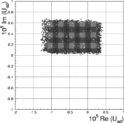
Figure 2: Phenomenological bounds on the FCNC coupling $U_{sd}$ with the $\varepsilon^{\prime}/\varepsilon$ hadronic parameters in set I.

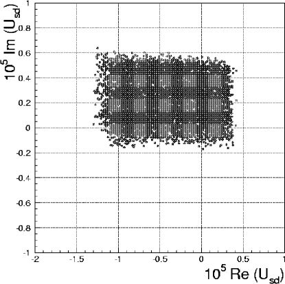
Figure 3: Phenomenological bounds on the FCNC coupling $U_{sd}$ with the $\varepsilon^{\prime}/\varepsilon$ hadronic parameters from set II.

In Figs. 2 and 3, we present a scatter plot of the allowed values of $U_{sd}$ in the general model with $n$ additional vector-like down quarks, although we must emphasize that this allowed region does not change at all even if we go to the more restricted case of a single VLdQ. We impose all the constraints described above, with the $\varepsilon^{\prime}/\varepsilon$ parameters from set I and set II in Fig. 2 and 3 respectively. In both approaches the bound for the real part is,

$$-1.3\times 10^{-5}<\mbox{Re}\{U_{sd}\}<4.0\times 10^{-6}$$ (18)

This constraint is directly obtained from Eq. (8) with the limit values of $\mbox{Re}(\lambda_{t}^{sd})$ which are $\mbox{Re}(\lambda_{t}^{sd})_{max}=-4.9\times 10^{-4}$ and $\mbox{Re}(\lambda_{t}^{sd})_{min}=-2.1\times 10^{-4}$ from Eq. (3) to ${\cal O}(\lambda^{5})$ for $\phi=\pi,0$ respectively. Therefore, this implies that the additional correlations among the parameters in the 1–VLdQ model are irrelevant for the $U_{sd}$ bound.

The constraints on the imaginary part of this coupling depend slightly on the adopted value for $B_{6}^{(1/2)}$. For set I, with $B_{6}^{(1/2)}=1.0\pm 0.2$, we can see that $U_{sd}$ is necessarily positive and does not reach the origin, indicating marginally the need of new physics for $\varepsilon^{\prime}/\varepsilon$. The allowed range is $1.0\times 10^{-7}<\mbox{Im}\{U_{ds}\}<6.5\times 10^{-6}$. On the other hand, in set II, we get an allowed area, $-1.5\times 10^{-6}<\mbox{Im}\{U_{ds}\}<6.0\times 10^{-6}$, including the SM as one of the possible points in agreement with the experimental results. This bounds are directly obtained from Eq. (12) with $\mbox{Im}(\lambda_{t}^{sd})_{max}=1.4\times 10^{-4}$ and $\mbox{Im}(\lambda_{t}^{sd})_{min}=6\times 10^{-5}$ assuming a $50\%$ error, which corresponds to the Gaussian errors that we use in this constraint. In view of these two different options to calculate $\varepsilon^{\prime}/\varepsilon$, we take a conservative bound on $\mbox{Im}(U_{sd})$ including both possibilities,

$$-1.5\times 10^{-6}<\mbox{Im}\{U_{sd}\}<6.5\times 10^{-6}$$ (19)

It is interesting to notice, that these bounds turn out to be much more stringent than the direct bounds on FCNC couplings usually quoted in the literature for VLdQ models [35]. This improvement is mainly due to the inclusion of the SM contributions that were completely neglected in the calculation of $\varepsilon_{K}$ in the bounds presented in [35], the improvement of the experimental results in $(K_{L}\rightarrow\mu^{+}\mu^{-})_{SD}$, $K^{+}\rightarrow\pi^{+}\nu\bar{\nu}$, and to the inclusion of the bound from $\varepsilon^{\prime}/\varepsilon$. In this way, our bounds basically agree with the general bounds in [20].

3.2 B physics constraints

In this section, we study the constraints on the $U_{bd}$ and $U_{bs}$ couplings from $B$ physics FCNC. In fact, the experimental information in the $B$ system is improving rapidly with the new results from $B$ factories and so, it is important to update the bounds on these FCNC couplings. In all the following processes, the choice of set I or set II to calculate $\varepsilon^{\prime}/\varepsilon$ has no relevant effects on the $U_{bd}$ and $U_{bs}$ couplings. Hence, we analyze the constraints making no distinction on the hadronic parameters used to calculate $\varepsilon^{\prime}/\varepsilon$. In first place, we concentrate on the constraints from $CP$ conserving processes and then we add the information from the $B^{0}$ $CP$ asymmetries.

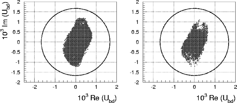
Figure 4: Constraints on the $U_{bd}$ coupling from $B_{d}$–$\bar{B}_{d}$ mixing in the $n$–VLdQ model (left) and in the 1–VLdQ model (right). The circle shows the bound obtained from the $B\to X_{d}l^{+}l^{-}$

The main $CP$ conserving processes constraining $U_{bd}$ and $U_{bs}$ are $\mbox{BR}(B\rightarrow X_{d,s}l^{+}l^{-})$ and $\Delta M_{B_{d,s}}$.

From the upper bound on $\mbox{BR}(B\rightarrow X_{s}l^{+}l^{-})\leq 4.2\times 10^{-5}$ [36] and assuming $\mbox{BR}(B\rightarrow X_{d}l^{+}l^{-})\leq\mbox{BR}(B\rightarrow X_{s}l^{+}l^{-})$ we have [23, 37],

$$\frac{\displaystyle{\Gamma\left(B\to X_{q}l^{+}l^{-}\right)}}{\displaystyle{\Gamma\left(B\to X_{c}e^{+}\nu_{e}\right)}} = \frac{\displaystyle{\alpha^{2}}}{\displaystyle{\pi^{2}\sin^{4}\theta_{W}}}\ \frac{\displaystyle{\left|Y_{0}\left(x_{t}\right)\lambda_{t}^{bq}\ +\ C_{U2Z}\ U_{bq}\right|^{2}}}{\displaystyle{|V_{cb}|^{2}f\left(m_{c}/m_{b}\right)}}\times$$ (20)

$$\left(2\sin^{4}\theta_{W}-\sin^{2}\theta_{W}+\frac{1}{4}\right)\leq 4\times 10^{-4}$$

with $f(z)=(1-8z^{2}+8z^{6}-z^{8}-24z^{4}\log z)$ a phase space factor due to the mass of the charm quark. From here we get,

$$\left|Y_{0}\left(x_{t}\right)\lambda_{t}^{bq}\ +\ C_{U2Z}\ U_{bq}\right|<0.15.$$ (21)

Replacing here $\lambda_{t}^{bd}\simeq A\lambda^{3}(1-\mu e^{-i\phi})+{\cal O}(\lambda^{5})\simeq 8\times 10^{-3}\ (1-0.4e^{-i\phi})$ with $Y_{0}\simeq 1$, it is clear that the $\lambda_{t}^{bd}$ contribution can be safely neglected and we get a bound $|U_{bd}|\leq 1.7\times 10^{-3}$. However, this is not true in the case of $\lambda_{t}^{bs}\simeq-A\lambda^{2}\simeq-0.040$ that shifts the $|U_{bs}|$ constraint to a circle of radius $1.7\times 10^{-3}$ centered in $(-0.040/92.7,0)$.

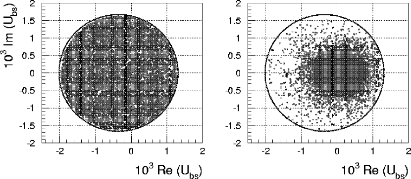
Figure 5: Constraints on the $U_{bs}$ coupling from $B\to X_{s}l^{+}l^{-}$ in the $n$–VLdQ model (left) and in the 1–VLdQ model (right).

Additionally, from $B$–$\bar{B}$ mixing we have [10, 11, 12]

$$M^{B_{q}}_{12}=\frac{\displaystyle{G_{F}^{2}M_{W}^{2}\eta_{B_{q}}B_{B_{q}}f_{B_{q}}^{2}m_{B_{q}}}}{\displaystyle{12\pi^{2}}}S_{0}\left(x_{t}\right)\ {\lambda_{t}^{bq}}^{2}\Delta_{bq},$$

$$\Delta_{bq}\ =\ 1\ -\ 3.3\ \frac{\displaystyle{U_{bq}}}{\displaystyle{\lambda_{t}^{bq}}}\ +\ 165\ \left(\frac{\displaystyle{U_{bq}}}{\displaystyle{\lambda_{t}^{bq}}}\right)^{2},$$ (22)

where the new parameters are defined in Ref. [23], and the mass difference $\Delta M_{B_{q}}=2\ |M^{B_{q}}_{12}|$. The experimental values for these observables are $\Delta M_{B_{d}}=\left(0.472\pm 0.017\right)\times 10^{12}\ \mbox{s}^{-1}$ and $\Delta M_{B_{s}}>14.9\times 10^{12}\ \mbox{s}^{-1}$ at $95\%$ C.L. [38, 39].

At this point, it is important to compare the bounds that can be obtained from the mass difference and the semileptonic decay. From $\mbox{BR}(B\rightarrow X_{d,s}l^{+}l^{-})$, we get a bound on $|\lambda_{t}^{bq}Y_{0}+C_{U2Z}U_{bq}|^{2}$ in Eq. (21), while from the mass difference, neglecting the linear term, we obtain a constraint on the combination $|(\lambda_{t}^{bq})^{2}S_{0}+4C_{U2Z}U_{bq}^{2}|$. Hence, it is clear that the relative size of the tree level FCNC with respect to the SM contribution is always bigger in the semileptonic decay due to the presence of an additional factor $C_{U2Z}\simeq-92.7$. Nevertheless, the experimental constraints from $\mbox{BR}(B\rightarrow X_{d,s}l^{+}l^{-})$ are still much larger than the typical SM prediction while the $\Delta M_{B_{d}}$ measurement is already saturated by the SM contribution. This implies that the $\Delta M_{B_{d}}$ constraint is more effective in the case of $U_{bd}$ and both experiments give rise to constraints of the same order of magnitude, dominating at the end the $\Delta M_{B_{d}}$ bound. This can be seen in Fig. 4, where we show the allowed region of the parameter space both in the general model with an arbitrary number of VLdQs and in the minimal model with a single VLdQ. In these figures, the constraint from $BR(B\rightarrow X_{d}l^{+}l^{-})$ is shown as a circle slightly shifted from the origin and a radius of $1.7\times 10^{-3}$. However, as we can see here, the bounds on $U_{bd}$ are $|\mbox{Re}\{U_{bd}\}|\leq 0.7\times 10^{-3}$ and $|\mbox{Im}\{U_{bd}\}|\leq 1.2\times 10^{-3}$, which are directly obtained from the $\Delta M_{B_{d}}$ constraint as the envelope of the curves $|(\lambda_{t}^{bd})^{2}S_{0}+4C_{U2Z}U_{bd}^{2}|$ with all the allowed values of $\lambda_{t}^{bd}$. Notice that already in this most constrained model, i.e. the model with a single VLdQ, the $U_{bd}$ coupling is only bounded by these processes and therefore we obtain the same bounds both in this case and in the general case with $n$ VLdQ.

In the case of the $U_{bs}$ coupling the situation is completely different. In first place $\Delta M_{B_{s}}$ has not been measured yet, and so only a lower bound on the mass difference is available which is not useful to set a constraint on $U_{bs}$. Moreover, it is easy to see from Eq. (22) that for similar values of $U_{bd}$ and $U_{bs}$, the FCNC effects on $\Delta M_{B_{s}}$ will be suppressed by a factor $(\lambda_{t}^{bd}/\lambda_{t}^{bs})^{2}\simeq\lambda^{2}$ when compared with the effects on $\Delta M_{B_{d}}$. This implies that in this model we cannot expect to observe the FCNC effects in $B_{s}$–$\bar{B}_{s}$ mixing . Hence, this coupling is only constrained by the upper bound on $\mbox{BR}(B\rightarrow X_{s}l^{+}l^{-})$. In Fig. 5, we show the constraint from $BR(B\rightarrow X_{s}l^{+}l^{-})$ as a circle slightly shifted from the origin, that implies an upper bound of $|U_{bs}|\leq 2\times 10^{-3}$ [37, 41] both in the general model with $n$ VLdQs and in the model with a single VLdQ. Similarly, the $b\to s\gamma$ branching ratio provides constraints of the same order of magnitude [42].

Despite these strong constraints from $CP$ conserving processes, the $CP$ asymmetries in $B$ decays are still very effective to constrain the $U_{bd}$ coupling [43, 44]. Recently, the arrival of the first measurements of the $B\to J/\psi K_{S}$ $CP$ asymmetry, $a_{J/\psi}$, from the $B$ factories has caused a great excitement in the high energy physics community.

$$\begin{array}[]{ll}&\\ a_{J/\psi}&=\\ &\\ \end{array}\left\{\begin{array}[]{ll}0.34\pm 0.20\pm 0.05&(\mbox{BaBar \cite[cite]{[\@@bibref{}{babar}{}{}]}})\\ 0.58^{+0.32+0.09}_{-0.34-0.10}&\left(\mbox{Belle \cite[cite]{[\@@bibref{}{belle}{}{}]}}\right)\\ 0.79^{+0.41}_{-0.44}&\left(\mbox{CDF \cite[cite]{[\@@bibref{}{CDF}{}{}]}}\right)\end{array}\right.$$ (23)

These values correspond to a world average of $a_{J/\psi}=0.51\pm 0.18$, that can be compared with the SM expectations of $0.59\leq a_{J/\psi}^{SM}=\sin(2\beta)\leq 0.82$ with $\beta=\mbox{arg}(-V_{cd}V_{cb}^{*}/(V_{td}V_{tb}^{*}))$. The errors are still too large to draw any firm conclusion. In fact, if we take the world average at $95\%$ C.L. we do not get any improvement over the constraints from $CP$ conserving processes. However, anticipating the improvement of the experimental errors from $B$ factories, we take the world average at 1 $\sigma$ level to see the effects on the $U_{bd}$ coupling. From Eq. (22), it is straightforward to obtain $a_{J/\psi}$ as,

$$a_{J/\psi}=\sin\left(2\beta-\mbox{arg}(\Delta_{bd})\right).$$ (24)

Using the world average at 1 $\sigma$ as the experimentally allowed range, we show in Fig. 6 the resulting region for the $U_{bd}$ coupling.

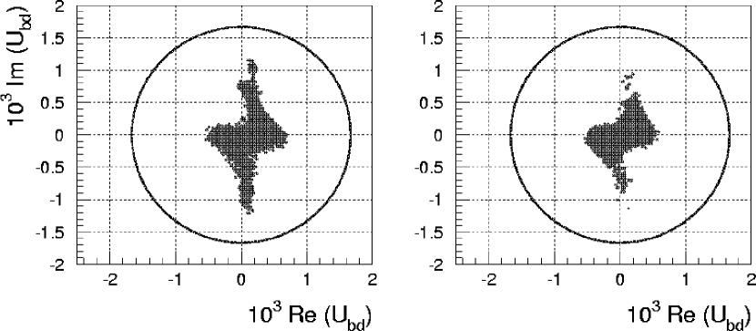
Figure 6: Allowed region for the $U_{bd}$ coupling requiring a value of $a_{J/\psi}$ asymmetry to reproduce the world average at 1 $\sigma$ in the $n$–VLdQ model (left) and 1–VLdQ model (right).

As we can see here, the $U_{bd}$ allowed region is sizeably modified from this constraint. The outer regions in the second and fourth quadrants are reduced while the central region corresponding to the SM remains filled; this situation represents an improvement over the analysis presented in Ref. [44]. Note that the results are essentially similar for the $n$–VLdQ and the 1–VLdQ cases. As we can see here, with the world average for the $a_{J/\psi}$ $CP$ asymmetry there is no need of new physics in the $U_{bd}$ sector.

4 Discovery potential in $B$ factories

As we have explained above, the present results in the $a_{J/\psi}$ asymmetry in Eq. (23) are not precise enough to make a definitive statement about the presence/absence of large new physics contributions in $B$ decays. Still, these measurements, and especially the BaBar value which is the most precise one, leave room for an asymmetry considerably smaller than the standard model expectations. The SM range is certainly outside the $1\sigma$ BaBar range but not outside the world average. This potential discrepancy is at the origin of several papers [48, 49] studying the implications of a small $a_{J/\psi}$ in the search of new physics. The papers in Ref. [48] provide general parametrizations of new physics contributions to $B$ mixing and decays. They essentially show that this possible mismatch among the measured value and the SM expectations may be due to the presence of new physics either directly in $B$ physics or in $K$ physics modifying indirectly the unitarity triangle fit. However, these papers do not provide a definite new physics example fulfilling this task. On the other hand, the two papers in Ref. [49] analyze SUSY models, where no sizeable effects in $B$ mixing and decays are generally expected and the unitarity triangle fit can be modified only through new SUSY contributions to $K$ physics. In the following, we show that a model with tree level FCNC from the mixing with vector-like quarks would be a natural candidate for a model with clear deviations from the SM expectations in $CP$ asymmetries, satisfying simultaneously all other experimental constraints.

Figure 7: Distribution of the values of $a_{J/\psi}$ for 95000 events in the $n$–VLdQ (left) and in the 1–VLdQ (right).

From the expression of $a_{J/\psi}$ in Eqs.(22) and (24), with $|\lambda_{t}^{bd}|\in[5\times 10^{-3},1.2\times 10^{-2}]$ and $|U_{bd}|\raise 1.29167pt\hbox{$\;<$\kern-7.5pt\raise-4.73611pt\hbox{$\sim\;$}}10^{-3}$, it is clear that $\mbox{arg}(\Delta_{bd})$ can be very large. Indeed, in the general model with an arbitrary number of VLdQ, there is no further influence on $U_{bd}$ from constraints on other elements of the mixing matrix. In fact, only the inequalities in Eq. (3) can restrict this coupling, however, given the bounds on $D^{2}_{i}$, they are almost inoperative in this case. Hence, all the points inside the allowed contour in Fig.4 are equally probable and any value of the asymmetry is possible with a comparable probability. Still, the especial geometry of this allowed region and the preferred orientation of $\lambda^{t}_{bd}$ slightly favors the SM range over other values. Furthermore, even in a more constrained model, as in the model with a single VLdQ large departures from the SM range are possible. The expected values for the asymmetry both in the $n$ VLdQs and in the 1 VLdQ model are shown in Fig. 7 as an histogram of the distribution of 95000 events satisfying all the constraints in the previous sections. As expected from the above discussion, in the general case all possible values of the asymmetry have similar probability. On the other hand, in the model with a single VLdQ, this distribution is clearly peaked on the SM range. Moderate deviations are rather frequent and larger departures are more rare but still possible for any value of the asymmetry.

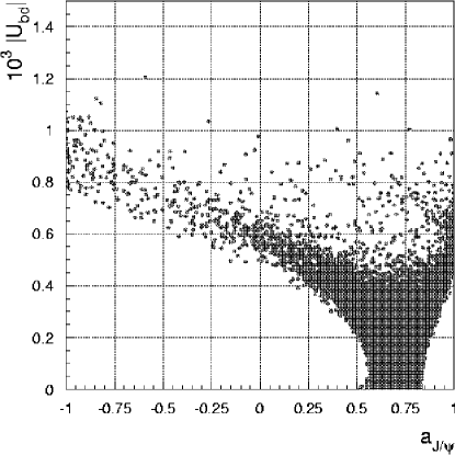
Figure 8: Correlation between the values of $a_{J/\psi}$ and $|U_{bd}|$ in the model with a single VLdQ.

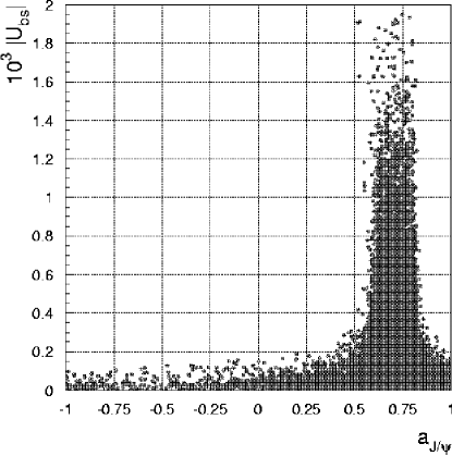
Figure 9: Correlation between the values of $a_{J/\psi}$ and $|U_{bs}|$ in the model with a single VLdQ.

In Figs. 8 and 9, we show, in the 1 VLdQ model the correlation of the possible values of the asymmetry with $|U_{bd}|$ and $|U_{bs}|$ respectively. Here, we see that the range $0.55\raise 1.29167pt\hbox{$\;<$\kern-7.5pt\raise-4.73611pt\hbox{$\sim\;$}}a_{J/\psi}\raise 1.29167pt\hbox{$\;<$\kern-7.5pt\raise-4.73611pt\hbox{$\sim\;$}}0.85$ corresponding to the SM expected range concentrates most of the events and can be reproduced with $|U_{bd}|=0$ and any allowed value of $|U_{bs}|$. However, for different values of the asymmetry there is a clear correlation between $a_{J/\psi}$ and the minimum value of $|U_{bd}|$ required to obtain this asymmetry. For instance to obtain an asymmetry below $0.5$, a $|U_{bd}|\geq 2\times 10^{-4}$ is needed. This required minimum is also true in the general model with an arbitrary number of VLdQs. Similarly, we see in Fig. 9 that these large values of $U_{bd}$ correspond to low values of $U_{bs}$ [11], however it is important to emphasize that this correlation is only true in the minimal model, but not in a model with an arbitrary number of VLdQs. To see this we show in Figs. 10 and 11 both in the $n$–VLdQ and in the 1–VLdQ models an scatter plot of $\mbox{Re}(U_{bd})$ versus $\mbox{Im}(U_{bd})$ and $\mbox{Re}(U_{bs})$ versus $\mbox{Im}(U_{bs})$ for an asymmetry corresponding to the BaBar result at $1\sigma$, $0.14\leq a_{J/\psi}\leq 0.54$ [45].

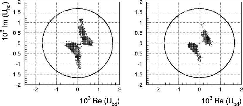
Figure 10: Allowed region for the $U_{bd}$ coupling consistent with the BaBar result for the $a_{J/\psi}$ asymmetry at 1 $\sigma$ in the $n$–VLdQ (left) and in the 1–VLdQ (right).

In this Fig. 10 we see that the great majority of the allowed points are in the range $1\times 10^{-4}\ (2\times 10^{-4})\raise 1.29167pt\hbox{$\;<$\kern-7.5pt\raise-4.73611pt\hbox{$\sim\;$}}\left|U_{bd}\right|\raise 1.29167pt\hbox{$\;<$\kern-7.5pt\raise-4.73611pt\hbox{$\sim\;$}}1.2\times 10^{-3}$, in the $n$-VLdQ (1–VLdQ) model, i.e. a large, non-vanishing $U_{bd}$ coupling is required to reproduce the BaBar asymmetry. In particular, this means that, within this model, a low CP asymmetry implies the presence of new physics in $b$–$d$ transitions. This conclusion would be unchanged in the general model. On the other hand, we see that, for these points, in the 1-VLdQ model, the coupling $U_{bs}$ is always restricted to the range $|U_{bs}|\raise 1.29167pt\hbox{$\;<$\kern-7.5pt\raise-4.73611pt\hbox{$\sim\;$}}3\times 10^{-4}$; hence all the allowed points have simultaneously high $\left|U_{bd}\right|$ and low $\left|U_{bs}\right|$. Indeed, it is easy to obtain in the 1–VLdQ model, from Eq. (3), the relation $U_{bd}U_{bs}^{*}=-U_{sd}D_{b}^{2}$. The region in the $U_{ds}$ plane does not change with the inclusion of the $a_{J/\psi}$ constraint, and then we still have, $|U_{sd}|\raise 1.29167pt\hbox{$\;<$\kern-7.5pt\raise-4.73611pt\hbox{$\sim\;$}}6\times 10^{-6}$ and $D_{b}^{2}\raise 1.29167pt\hbox{$\;<$\kern-7.5pt\raise-4.73611pt\hbox{$\sim\;$}}0.009$. Taking into account that a low $a_{J/\psi}$ requires $|U_{bd}|\geq 2\times 10^{-4}$, this clearly implies an absolute upper bound, $|U_{bs}|\raise 1.29167pt\hbox{$\;<$\kern-7.5pt\raise-4.73611pt\hbox{$\sim\;$}}3\times 10^{-4}$. Therefore, for this set of points, we can not expect a new-physics contribution in the $b\to s$ transition. However, this relation is not valid in the $n$–VLdQ model and therefore this correlation is lost as can be seen in Fig.11.

Also in Fig. 10, we find a few points ($\simeq 0.1\%$ of the points) which have simultaneously $|U_{bs}|\raise 1.29167pt\hbox{$\;>$\kern-7.5pt\raise-4.73611pt\hbox{$\sim\;$}}1\times 10^{-3}$ and $|U_{bd}|\raise 1.29167pt\hbox{$\;<$\kern-7.5pt\raise-4.73611pt\hbox{$\sim\;$}}3\times 10^{-5}$. This second class of points is only possible in the vicinity of the SM and they disappear if the value of the asymmetry is reduced to $a_{J/\psi}\raise 1.29167pt\hbox{$\;<$\kern-7.5pt\raise-4.73611pt\hbox{$\sim\;$}}0.52$ .

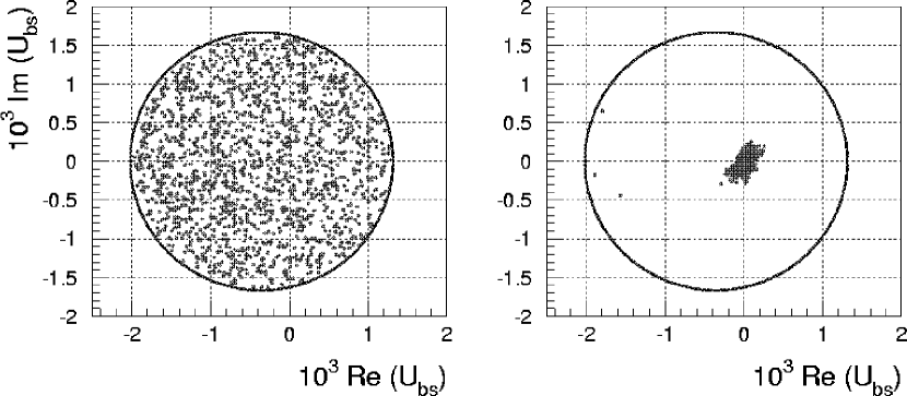
Figure 11: Allowed region for the $U_{bs}$ coupling consistent with the BaBar result for the $a_{J/\psi}$ asymmetry at 1 $\sigma$ in the $n$–VLdQ (left) and in the 1–VLdQ (right).

Therefore, we can conclude that in a model with a single VLdQ a low $CP$ asymmetry $a_{J/\psi}\leq 0.52$ implies $|U_{bd}|\geq 2\times 10^{-4}$ and simultaneously $|U_{bs}|\leq 3\times 10^{-4}$. On the contrary, in a general model with an arbitrary number of VLdQs, we still have $|U_{bd}|\geq 2\times 10^{-4}$, but this has no influence on the $U_{bs}$ coupling, and it is only constrained by the $B\to X_{s}l\bar{l}$ branching ratio.

At this point, it is very interesting to examine the predicted branching ratios of the decays $B\to X_{d,s}l\bar{l}$ for this set of points. From Fig. 10, where we have included the circle corresponding to the experimental bounds in these decays, it is clear that we can also expect a very large contribution to $B\to X_{d}l\bar{l}$. In this case, the branching ratios for the $X_{d}$ decays are strongly enhanced from the SM prediction, reaching values of $1.0\times 10^{-6}\leq BR\left(B\rightarrow X_{d}l^{+}l^{-}\right)\leq 1.8\times 10^{-5}$ and $6.0\times 10^{-5}\leq BR\left(B\rightarrow X_{d}\nu\bar{\nu}\right)\leq 1.0\times 10^{-4}$. While, on the other hand, the low values of $U_{bs}$ imply that the $X_{s}$ decays remain roughly at the SM value. Conversely, in the points with small $U_{bd}$ and large $U_{bs}$, there is no sizeable departure from the SM expectations in $B\to X_{d}l\bar{l}$ and the $X_{s}$ decays are now close to the experimental upper range. Namely, we obtain, for the points to the right of Fig. 11, with $Re\left(U_{bs}\right)\simeq 1\times 10^{-4}$, $BR\left(B\rightarrow X_{s}l^{+}l^{-}\right)\simeq 2.7\times 10^{-5}$ to be compared with the experimental upper bounds of $BR\left(B\rightarrow X_{s}l^{+}l^{-}\right)\leq 4.2\times 10^{-5}$. However, this possibility is only marginal in the $1\sigma$ BaBar range for the minimal model with a single VLdQ. In any case in the general model, the possibility of large $U_{bs}$ couplings is again open. For analysis of the phenomenological effects of this coupling in radiative $b\to s\gamma$ decays, $B_{s}$–$\bar{B}_{s}$ mixing and rare decays in a slightly different context, see Refs. [40, 41, 42].

5 Conclusions

In this work, we have updated the constraints on tree level FCNC couplings in the framework of a theory with $n$ isosinglet vector-like down quarks. The inclusion of the constraints from $(K_{L}\to\mu^{+}\mu^{-})_{SD}$, $\varepsilon^{\prime}/\varepsilon$, $\varepsilon_{K}$ and $K\to\pi\nu\bar{\nu}$ has allowed to improve sizeably the bound on the $U_{sd}$ coupling. The precise range of allowed values for this coupling depends strongly on the hadronic input in the calculation of $\varepsilon^{\prime}/\varepsilon$. Our summary in Table 1 includes the main theoretical approaches [20, 24, 25, 26, 27, 28, 29, 30, 31]. In the near future, $K^{+}\to\pi^{+}\nu\bar{\nu}$ will be quite useful to further constrain $U_{sd}$ without large theoretical uncertainties.

We have calculated the constraints on $U_{bd}$ and $U_{bs}$ from $\Delta M_{B_{d}}$, $B\to X_{s,d}l\bar{l}$ and the $B\to J/\psi K_{S}$ $CP$ asymmetry. In Table 1, we summarize our results on these bounds without the additional constraint from the $B\to J/\psi K_{S}$ $CP$. Note that all these bounds on $U_{bq}$ are independent of the hadronic inputs in $\varepsilon^{\prime}/\varepsilon$.

Re $\{U_{sd}\}$	$\geq-1.3\times 10^{-5}$	$\leq 4.0\times 10^{-6}$
Im $\{U_{sd}\}$	$\geq-1.5\times 10^{-6}$	$\leq 6.5\times 10^{-6}$
$|\mbox{Re}\{U_{bd}\}|$	$\leq 7\times 10^{-4}$
$|\mbox{Im}\{U_{bd}\}|$	$\leq 1.2\times 10^{-3}$
$|U_{bs}|$	$\leq 2\times 10^{-3}$

Table 1: Constraints on the tree level FCNC couplings from rare processes in the $K$ and $B$ systems.

In addition, we have shown that the $B\to J/\psi K_{S}$ $CP$ asymmetry is especially sensitive to the presence of a $U_{bd}$ FCNC coupling. In this regard, we have shown that the 1 $\sigma$ value of the world average is already able to exclude half of the allowed region for the $U_{bd}$ coupling. However, due to the still large experimental errors this constraint has a small effect at $95\%$ C.L. Assuming a low value of the $a_{J/\psi}$ asymmetry below $\sim 0.52$ (following BaBar range at 1 $\sigma$) we have shown that, in models with $n$ VLdQs, tree-level FCNC in the $b$–$d$ sector are mandatory. The FCNC coupling $U_{bd}$ is required to be greater than $1\times 10^{-4}$, rising to $2\times 10^{-4}$ in the 1–VLdQ model. The $U_{bs}$ coupling in the general model is bounded by $2\times 10^{-3}$, although for the 1–VLdQ model the bound goes down to $3\times 10^{-4}$.

Therefore, a clear favorable scenario for these models would be to find simultaneously a low $a_{J/\psi}$ (below $\sim 0.5$) and a large $\mbox{BR}(B_{d}\to X_{d}l\bar{l})$, at least one order of magnitude bigger than the SM expectations. Values of $\mbox{BR}(B_{d}\to X_{s}l\bar{l})$ close to the present experimental bounds are still possible in the $n$–VLdQ model. Nevertheless, in the 1–VLdQ model these BR are expected to be similar to the SM values. In summary, this $a_{J/\psi}$ $CP$ asymmetry, together with the rare decays $B\to X_{s,d}l\bar{l}$ and $K\to\pi\nu\bar{\nu}$ are the best options to further constraint the FCNC tree level couplings or to discover the presence of vector-like quarks in the low energy spectrum as suggested by GUT theories or models of large extra dimensions at the TeV scale.

References

- [1] S. L. Glashow, J. Iliopoulos and L. Maiani, Phys. Rev. D 2 (1970) 1285.
- [2] M. K. Gaillard and B. W. Lee, Phys. Rev. D 10 (1974) 897.
-
[3]
J. Ellis and D. V. Nanopoulos,
Phys. Lett. B 110 (1982) 44;
R. Barbieri and R. Gatto, Phys. Lett. B 110 (1982) 211;
S. Bertolini, F. Borzumati, A. Masiero and G. Ridolfi, Nucl. Phys. B 353 (1991) 591;
F. Gabbiani, E. Gabrielli, A. Masiero and L. Silvestrini, Nucl. Phys. B 477 (1996) 321 [hep-ph/9604387];
A. Masiero and O. Vives, hep-ph/0104027 and references therein. -
[4]
M. Bando and T. Kugo,
Prog. Theor. Phys. 101 (1999) 1313
[hep-ph/9902204].
M. Bando, T. Kugo and K. Yoshioka, Prog. Theor. Phys. 104 (2000) 211 [hep-ph/0003220];
M. Obara, G. Cho, M. Nagashima, A. Sugamoto, hep-ph/0105287. -
[5]
N. Arkani-Hamed, S. Dimopoulos and G. Dvali,
Phys. Lett. B 429 (1998) 263
[hep-ph/9803315];
L. Randall and R. Sundrum, Phys. Rev. Lett. 83 (1999) 3370 [hep-ph/9905221]; -
[6]
For phenomenology of FCNC in models with large extra dimension, see:
A. Delgado, A. Pomarol and M. Quiros, JHEP 0001 (2000) 030 [hep-ph/9911252].
F. del Aguila and J. Santiago, Phys. Lett. B 493 (2000) 175 [hep-ph/0008143].
S. J. Huber and Q. Shafi, Phys. Lett. B 498 (2001) 256 [hep-ph/0010195];
N. Rius and V. Sanz, hep-ph/0103086;
H. Davoudiasl and T. G. Rizzo, hep-ph/0104199;
S. J. Huber and Q. Shafi, hep-ph/0104293. - [7] G. Barenboim, F. J. Botella and O. Vives, work in progress.
-
[8]
F. del Aguila and J. Cortes,
Phys. Lett. B156 (1985) 243;
G. C. Branco and L. Lavoura, Nucl. Phys. B278 (1986) 738;
F. del Aguila, M. K. Chase and J. Cortes, Nucl. Phys. B271 (1986) 61;
Y. Nir and D. J. Silverman, Phys. Rev. D42 (1990) 1477;
D. Silverman, Phys. Rev. D45 (1992) 1800;
G. C. Branco, T. Morozumi, P. A. Parada and M. N. Rebelo, Phys. Rev. D48 (1993) 1167;
W. Choong and D. Silverman, Phys. Rev. D49 (1994) 2322;
V. Barger, M. S. Berger and R. J. Phillips, Phys. Rev. D52 (1995) 1663 [hep-ph/9503204];
D. Silverman, Int. J. Mod. Phys. A11 (1996) 2253 [hep-ph/9504387];
M. Gronau and D. London, Phys. Rev. D55 (1997) 2845 [hep-ph/9608430];
F. del Aguila, J. A. Aguilar-Saavedra and G. C. Branco, Nucl. Phys. B510 (1998) 39 [hep-ph/9703410]. - [9] L. Lavoura and J. P. Silva, Phys. Rev. D47 (1993) 1117.
- [10] G. Barenboim, F. J. Botella, G. C. Branco and O. Vives, Phys. Lett. B422 (1998) 277 [hep-ph/9709369].
- [11] G. Barenboim, F. J. Botella and O. Vives, Phys. Rev. D64 (2001) 015007 [hep-ph/0012197].
- [12] G. Barenboim and F. J. Botella, Phys. Lett. B433 (1998) 385 [hep-ph/9708209].
- [13] J. Roldan, F. J. Botella and J. Vidal, Phys. Lett. B283 (1992) 389.
- [14] F. J. Botella and L. Chau, Phys. Lett. B168 (1986) 97.
- [15] L. Chau and W. Keung, Phys. Rev. Lett. 53 (1984) 1802.
- [16] D. E. Groom et al., Eur. Phys. J. C15 (2000) 1.
- [17] L. Wolfenstein, Phys. Rev. Lett. 51 (1983) 1945.
-
[18]
R. Barate et al. [ALEPH Collaboration],
Phys. Lett. B465 (1999) 349;
P. Abreu et al. [DELPHI Collaboration], Phys. Lett. B439 (1998) 209;
M. Bargiotti et al., Riv. Nuovo Cim. 23N3 (2000) 1 [hep-ph/0001293]. - [19] F. del Aguila, J. A. Aguilar-Saavedra and R. Miquel, Phys. Rev. Lett. 82 (1999) 1628 [hep-ph/9808400].
- [20] A. J. Buras and L. Silvestrini, Nucl. Phys. B546 (1999) 299 [hep-ph/9811471].
-
[21]
D. Gomez Dumm and A. Pich,
Phys. Rev. Lett. 80 (1998) 4633
[hep-ph/9801298];
G. D’Ambrosio, G. Isidori and J. Portoles, Phys. Lett. B423 (1998) 385 [hep-ph/9708326]. - [22] T. Inami and C. S. Lim, Prog. Theor. Phys. 65 (1981) 297.
- [23] A. J. Buras and R. Fleischer, Report No. TUM-HEP-275-97, hep-ph/9704376.
-
[24]
M. Ciuchini, E. Franco, L. Giusti, V. Lubicz and G. Martinelli,
Report No. ROME-99-1268,
hep-ph/9910237;
M. Ciuchini and G. Martinelli, Nucl. Phys. Proc. Suppl. 99 (2001) 27 [hep-ph/0006056];
S. Bosch, A. J. Buras, M. Gorbahn, S. Jager, M. Jamin, M. E. Lautenbacher and L. Silvestrini, Nucl. Phys. B565 (2000) 3 [hep-ph/9904408]. - [25] A. J. Buras, hep-ph/0101336.
-
[26]
T. Hambye, G. O. Kohler, E. A. Paschos, P. H. Soldan and W. A. Bardeen,
Phys. Rev. D 58 (1998) 014017
[hep-ph/9802300];
T. Hambye, G. O. Kohler and P. H. Soldan, Eur. Phys. J. C 10 (1999) 271 [hep-ph/9902334]. -
[27]
S. Bertolini, J. O. Eeg, M. Fabbrichesi and E. I. Lashin,
Nucl. Phys. B514 (1998) 93
[hep-ph/9706260];
S. Bertolini, M. Fabbrichesi and J. O. Eeg, Rev. Mod. Phys. 72 (2000) 65 [hep-ph/9802405]. -
[28]
E. Pallante and A. Pich,
Phys. Rev. Lett. 84 (2000) 2568
[hep-ph/9911233];
E. Pallante, A. Pich and I. Scimemi, hep-ph/0105011. -
[29]
J. Bijnens and J. Prades,
JHEP 0006 (2000) 035
[hep-ph/0005189];
J. Bijnens and J. Prades, JHEP 0001 (2000) 002 [hep-ph/9911392];
J. Bijnens and J. Prades, Nucl. Phys. Proc. Suppl. 96 (2001) 354 [hep-ph/0010008]. - [30] S. Narison, Nucl. Phys. B 593 (2001) 3 [hep-ph/0004247].
- [31] J. F. Donoghue and E. Golowich, Phys. Lett. B 478 (2000) 172 [hep-ph/9911309].
- [32] G. Buchalla and A. J. Buras, Phys. Rev. D 54 (1996) 6782 [hep-ph/9607447].
-
[33]
S. Adler et al. [E787 Collaboration],
Phys. Rev. Lett. 79 (1997) 2204
[hep-ex/9708031];
S. Adler et al. [E787 Collaboration], Phys. Rev. Lett. 84 (2000) 3768 [hep-ex/0002015]. - [34] T. K. Komatsubara [E787 Collaboration], hep-ex/9905014.
-
[35]
Y. Nir and D. J. Silverman,
Phys. Rev. D 42 (1990) 1477;
Y. Grossman, Y. Nir and R. Rattazzi, hep-ph/9701231. - [36] S. Glenn et al. [CLEO Collaboration], Phys. Rev. Lett. 80 (1998) 2289 [hep-ex/9710003].
- [37] G. Buchalla, G. Hiller and G. Isidori, Phys. Rev. D 63 (2001) 014015 [hep-ph/0006136].
- [38] A. Stocchi, hep-ph/0010222.
- [39] A. Ali and D. London, Eur. Phys. J. C 18 (2001) 665 [hep-ph/0012155].
-
[40]
M. Aoki, M. Nagashima and N. Oshimo,
hep-ph/0104063;
M. Aoki, G. Cho, M. Nagashima and N. Oshimo, hep-ph/0102165. - [41] M. R. Ahmady, M. Nagashima and A. Sugamoto, hep-ph/0105049.
-
[42]
C. V. Chang, D. Chang and W. Keung,
Phys. Rev. D 61 (2000) 053007;
M. Aoki, E. Asakawa, M. Nagashima, N. Oshimo and A. Sugamoto, Phys. Lett. B 487 (2000) 321 [hep-ph/0005133]. - [43] G. Barenboim, G. Eyal and Y. Nir, Phys. Rev. Lett. 83 (1999) 4486 [hep-ph/9905397].
- [44] G. Eyal and Y. Nir, JHEP 9909 (1999) 013 hep-ph/9908296.
- [45] B. Aubert et al. [BaBar Collaboration], Report No. SLAC-PUB-8540, hep-ex/0008048;
- [46] H. Aihara [Belle Collaboration], Belle note 353, hep-ex/0010008.
- [47] T. Affolder et al., CDF Collaboration, Phys. Rev. D61 (2000) 072005 [hep-ex/9909003].
-
[48]
J. P. Silva and L. Wolfenstein,
Phys. Rev. D 63 (2001) 056001
[hep-ph/0008004];
G. Eyal, Y. Nir and G. Perez, JHEP 0008 (2000) 028 hep-ph/0008009;
Z. Xing, hep-ph/0008018;
A. J. Buras and R. Buras, Phys. Lett. B 501 (2001) 223 [hep-ph/0008273]. -
[49]
A. Masiero and O. Vives,
Phys. Rev. Lett. 86 (2001) 26
[hep-ph/0007320];
A. Masiero, M. Piai and O. Vives, Report No. FTUV-12-08, hep-ph/0012096.