1 Introduction

There exists a lot of theoretical interest in measuring the branching ratios for the inclusive radiative decays $B\to X_{s}\gamma$ and $B\to X_{d}\gamma$. The corresponding exclusive radiative decays $B\to K^{*}\gamma$ and $B\to\rho\gamma$, and related decays involving higher $K^{*}$ and $\rho$-resonances, are experimentally more tractable but theoretically less clean. In particular, the form factors entering in these decays have to be determined from a non-perturbative approach such as lattice-QCD or QCD sum rules. Alternatively, these form factors can be related to the ones in the semileptonic decays $B\to\rho\ell\nu_{\ell}$ using heavy quark symmetry and determined from data on the semileptonic decays. As the heavy quark symmetry is broken by perturbative QCD and non-perturbative power corrections, these effects will have to be taken into account at some level. This should enable us in principle to predict the branching ratios in radiative decays in a theoretically controlled way. In the Standard Model (SM), measurements of the radiative decays in question, as well as their semileptonic counterparts $B\to(K,K^{*},\pi,\rho)\ell^{+}\ell^{-}$, will constrain the matrix elements of the Cabibbo-Kobayashi-Maskawa (CKM) matrix [1]. In particular, the ratios of the branching ratios ${\cal B}(B\to\rho\gamma)/{\cal B}(B\to K^{*}\gamma)$ would provide independent and complementary information on the CKM matrix element ratio $|V_{td}/V_{ts}|$. Likewise, the isospin-violating ratios $\Delta^{\pm 0}=\Gamma(B^{\pm}\to\rho^{\pm}\gamma)]/[2\Gamma(B^{0}(\bar{B}^{0})\to\rho^{0}\gamma)]-1$ and the CP-asymmetry in the rate difference ${\cal A}_{\rm CP}(\rho^{\pm}\gamma)=[\Gamma(B^{-}\to\rho^{-}\gamma)-\Gamma(B^{+}\to\rho^{+}\gamma)]/[\Gamma(B^{-}\to\rho^{-}\gamma)+\Gamma(B^{+}\to\rho^{+}\gamma)]$ will determine the angle $\alpha$, which is one of the three inner angles of the CKM-unitarity triangle. They are also sensitive to the presence of physics beyond the SM, such as supersymmetry [2, 3]. It is therefore imperative to firm up theoretical predictions in exclusive decays $B\to V\gamma^{(*)}$, with $V=\rho$ or $K^{*}$, for precision tests of the SM and to interpret data for possible new physics effects in these decays.

To compute the branching ratios reliably, one needs to calculate at least the explicit $O(\alpha_{s})$ improvements to the lowest order decay widths and take into account the leading power corrections in a well-defined theoretical framework, such as the heavy quark effective theory (HQET). More specifically, theoretically improved radiative decay widths for $B\to V\gamma$, require the calculation of the renormalization group effects in the appropriate Wilson coefficients in the effective Hamiltonian [4], an explicit $O(\alpha_{s})$ calculation of the matrix elements involving the hard vertex corrections [5, 6, 7], annihilation contributions [8, 9, 10], which are more important in the decays $B\to\rho\gamma$, and the so-called hard-spectator contributions involving (virtual) hard gluon radiative corrections off the spectator quarks in the $B$-, $K^{*}$-, and $\rho$-mesons [11, 12]. These corrections will shift the theoretical branching ratios and induce CP-asymmetries in the decay rates, where the latter are expected to be measurable only in the CKM-suppressed decays $B\to\rho\gamma$ in the SM. In addition, the annihilation and the hard gluon radiative corrections explicitly break isospin symmetry, leading generically to non-zero values for $\Delta^{\pm 0}$ in $B\to\rho\gamma$ decays, and to a lesser extent also for the $B\to K^{*}\gamma$ decays. While the former have been calculated in the lowest order in Refs. [8, 9], and the explicit $O(\alpha_{s})$ corrections to the leading-twist (twist-two) annihilation amplitudes are found to vanish in the chiral limit [10], the commensurate contributions from the hard spectator diagrams have to be included in the complete $O(\alpha_{s})$-improved estimates. In this paper we compute these corrections to the leading-twist meson distribution amplitudes, borrowing techniques from the so-called Large Energy Effective Theory (LEET) [13, 14]. In doing this, we correct several errors in the derivation of the decay widths for $B\to\rho\gamma$, presented in the earlier version of this paper, and discuss in addition the decays $B\to K^{*}\gamma$ at some length in view of its current experimental interest. In a closely related context, a part of these corrections were calculated some time ago by Beneke and Feldmann [12]. With the remaining contribution of the hard spectator corrections presented here, and in the meanwhile also reported by Beneke, Feldmann and Seidel [15], and by Bosch and Buchalla [16], the decay rates for $B\to K^{*}\gamma$ and $B\to\rho\gamma$ are now quantified in the LEET approach, up to and including the NLO corrections in $\alpha_{s}$ and to leading power in $\Lambda_{\rm QCD}/M$, where $M$ is the $B$-meson mass, in the leading-twist approximation. These predictions have to be confronted with data, which we undertake at some length in this paper.

We use the $O(\alpha_{s})$-improved estimates for the decay rate for $B\to K^{*}\gamma$, presented here, the corresponding theoretical results for the inclusive decay rate for $B\to X_{s}\gamma$, obtained in Refs. [4, 17, 18], and current data on the branching ratios for $B\to K^{*}\gamma$ [19, 20, 21] and $B\to X_{s}\gamma$ [22, 23, 24] to determine the form factor $\xi_{\perp}^{(K^{*})}(0)$ in the LEET approach. This yields $\xi_{\perp}^{(K^{*})}(0)=0.25\pm 0.04$, which is similar, though not identical, to the result $\xi_{\perp}^{(K^{*})}(0)=0.24\pm 0.06$ obtained in Ref. [15] in the same framework, using the experimental branching ratio for $B\to K^{*}\gamma$ only. Relating the LEET-theory form factor $\xi_{\perp}^{(K^{*})}(0)$ to the full QCD form factor $T_{1}^{(K^{*})}(0)$, with the help of the $O(\alpha_{s})$-relation calculated in Ref. [12], yields $T_{1}^{(K^{*})}(0)=0.27\pm 0.04$. This is to be compared with a typical estimate in the light-cone QCD (LC-QCD) sum rule, $T_{1}^{(K^{*})}(0)=0.38\pm 0.05$ [25, 26] and from the lattice QCD simulations $T_{1}^{(K^{*})}(0)=0.32^{+0.04}_{-0.02}$ [27]. Thus, the form factor $T_{1}^{(K^{*})}(0)$ in the LEET approach is found to be smaller compared to the values obtained in the other two methods. At this stage, the source of this mismatch is not well understood.

What concerns the decay $B\to\rho\gamma$, we combine the current determination of $\xi_{\perp}^{(K^{*})}(0)$ in the LEET approach with an estimate of the SU(3)-breaking effects in the form factors, using a light-cone QCD sum rule result for this purpose, $\xi_{\perp}^{(\rho)}/\xi_{\perp}^{(K^{*})}=T_{1}^{(\rho)}(0)/T_{1}^{(K^{*})}(0)\simeq 0.76\pm 0.06$ [28], yielding $\xi_{\perp}^{(\rho)}=0.19\pm 0.04$. This allows us to calculate the branching ratios for the decays $B^{0}\to\rho^{0}\gamma$, $B^{+}\to\rho^{+}\gamma$ and their charge conjugates. However, as we show by explicit calculations in this paper, a parametrically more stable quantity for this purpose is the ratio ${\cal B}(B\to\rho\gamma)/{\cal B}(B\to K^{*}\gamma)$. Theoretically, this ratio can be expressed as

$$\frac{{\cal B}_{\rm th}(B\to\rho\gamma)}{{\cal B}_{\rm th}(B\to K^{*}\gamma)}=S_{\rho}\left|\frac{V_{td}}{V_{ts}}\right|^{2}\frac{(1-m_{\rho}^{2}/M^{2})^{3}}{(1-m_{K^{*}}^{2}/M^{2})^{3}}\,\zeta^{2}\,\left[1+\Delta R(\rho/K^{*})\right],$$

where $\zeta=\xi_{\perp}^{(\rho)}(0)/\xi_{\perp}^{(K^{*})}(0)$ is the ratio of the HQET/LEET form factors, $S_{\rho}=1(1/2)$ is the isospin weight for the $\rho^{\pm}$- ($\rho^{0}$-) meson, and the dominant dependence on the CKM matrix elements is made explicit. We calculate $\Delta R(\rho/K^{*})$, to leading order in $\alpha_{s}$ and $\Lambda_{\rm QCD}/M$, including the leading order annihilation contributions in $B\to\rho\gamma$ decays, and study its sensitivity to the underlying input parameters. Knowing $\Delta R(\rho/K^{*})$ and $\zeta$, the branching ratio for $B\to\rho\gamma$ can be predicted in terms of the already known branching ratios for $B\to K^{*}\gamma$. Averaged over the charge conjugates, we find $\bar{\cal B}_{\rm th}(B^{\pm}\to\rho^{\pm}\gamma)=[0.91\pm 0.33{(\rm th)}\pm 0.11{\rm(exp)}]\times 10^{-6}$ and $\bar{\cal B}_{\rm th}(B^{0}/\bar{B}^{0}\to\rho^{0}\gamma)=[0.50\pm 0.18{(\rm th)}\pm 0.04{\rm(exp)}]\times 10^{-6}$, where the theoretical uncertainty is dominated by the current dispersion on the CKM parameters and the meson wave functions. The experimental uncertainty enters through the present measurements of the branching ratios for $B\to K^{*}\gamma$. The isospin-violating ratios $\Delta^{\pm 0}$ and the charge conjugate averaged ratio $\Delta=(\Delta^{+0}+\Delta^{-0})/2$ are also calculated to the stated level of theoretical accuracy. The resulting corrections are found to be small in $\Delta$, in particular in the allowed CKM parameter range determined from the CKM unitarity fits in the SM.

Finally, we compute the leading order CP-asymmetry ${\cal A}_{\rm CP}(\rho^{\pm}\gamma)$ involving the decays $B^{\pm}\to\rho^{\pm}\gamma$ and the direct CP-asymmetry component in ${\cal A}_{\rm CP}(\rho^{0}\gamma)$, involving the decays $B^{0}/\bar{B}^{0}\to\rho^{0}\gamma$. These CP-asymmetries arise due to the interference of the various penguin amplitudes which have clashing weak phases, with the required strong interaction phase provided by the ${\cal O}(\alpha_{s})$ corrections entering the penguin amplitudes via the Bander-Silverman-Soni (BSS) mechanism [29]. We find that the hard spectator corrections significantly reduce the CP-asymmetries calculated from the vertex contribution alone in $B\to\rho\gamma$ decays, qualitatively in line with the observation made by Bosch and Buchalla [16]. However, this cancellation, and the resulting CP asymmetries, depend rather sensitively on the ratio of the quark masses $m_{c}/m_{b}$ and the annihilation contributions. This parametric dependence, combined with the scale dependence of ${\cal A}_{\rm CP}(\rho^{\pm}\gamma)$ and ${\cal A}_{\rm CP}(\rho^{0}\gamma)$, also discussed in Ref. [16], makes the prediction of direct CP-asymmetries rather unreliable, as we show explicitly in this paper.

This paper is organized as follows: In section 2, we introduce the underlying theoretical framework (LEET) and the relations involving the $B\to V$ ($V=\rho,K^{*}$) form factors resulting from the LEET symmetry, and sketch the explicit $O(\alpha_{s})$-breaking of these relations. The hard scattering amplitude involving the spectator diagrams in $B\to V\gamma$ decays are calculated in section 3. Explicit forms of the $O(\alpha_{s})$-corrected matrix elements for these decays are given in section 4. Numerical results for the branching ratios for $B\to K^{*}\gamma$ and $B\to\rho\gamma$ are presented in section 5. Isospin-violating ratios and the charge conjugate averaged ratio $\Delta$ for the decays $B\to\rho\gamma$, and the CP-violating asymmetry ${\cal A}_{\rm CP}(\rho^{\pm}\gamma)$ and the direct CP-asymmetry component in ${\cal A}_{\rm CP}(\rho^{0}\gamma)$ are given in section 6. We conclude with a brief summary and some concluding remarks in section 7.

2 LEET Symmetry and Symmetry Breaking in
Perturbative QCD

For the sake of definiteness, we shall work out explicitly the decays $B\to\rho\gamma$; the differences between these and the decays $B\to K^{*}\gamma$ lie mainly in the CKM matrix elements and in the wave functions of the final-state hadrons, and they will be specified in sections 4 and 5. The effective Hamiltonian for the $B\to\rho\gamma$ decays (equivalently $b\to d\gamma$ decay) at the scale $\mu=O(m_{b})$, where $m_{b}$ is the $b$-quark mass, is given by

$${\cal H}_{\rm eff} = \frac{G_{F}}{\sqrt{2}}\,\left\{V_{ub}V_{ud}^{*}\,\left[C_{1}^{(u)}(\mu)\,{\cal O}_{1}^{(u)}(\mu)+C_{2}^{(u)}(\mu)\,{\cal O}_{2}^{(u)}(\mu)\right]\right.$$

$$\qquad+\,V_{cb}V_{cd}^{*}\,\left[C_{1}^{(c)}(\mu)\,{\cal O}_{1}^{(c)}(\mu)+C_{2}^{(c)}(\mu)\,{\cal O}_{2}^{(c)}(\mu)\right]$$

$$\qquad-\,\left.V_{tb}V_{td}^{*}\,\left[C_{7}^{\rm eff}(\mu)\,{\cal O}_{7}(\mu)+C_{8}^{\rm eff}(\mu)\,{\cal O}_{8}(\mu)\right]+\ldots\right\},$$

where we have shown the contributions which will be important in our calculations. Operators ${\cal O}_{1}^{(q)}$ and ${\cal O}_{2}^{(q)}$, $(q=u,c)$, are the standard four-fermion operators:

$${\cal O}_{1}^{(q)}=(\bar{d}_{\alpha}\gamma_{\mu}(1-\gamma_{5})q_{\beta})\,(\bar{q}_{\beta}\gamma^{\mu}(1-\gamma_{5})b_{\alpha}),\qquad{\cal O}_{2}^{(q)}=(\bar{d}_{\alpha}\gamma_{\mu}(1-\gamma_{5})q_{\alpha})\,(\bar{q}_{\beta}\gamma^{\mu}(1-\gamma_{5})b_{\beta}),$$ (2.2)

and ${\cal O}_{7}$ and ${\cal O}_{8}$ are the electromagnetic and chromomagnetic penguin operators, respectively:

$${\cal O}_{7}=\frac{em_{b}}{8\pi^{2}}\,(\bar{d}_{\alpha}\sigma^{\mu\nu}(1+\gamma_{5})b_{\alpha})\,F_{\mu\nu},\qquad{\cal O}_{8}=\frac{g_{s}m_{b}}{8\pi^{2}}\,(\bar{d}_{\alpha}\sigma^{\mu\nu}(1+\gamma_{5})T^{a}_{\alpha\beta}b_{\beta})\,G^{a}_{\mu\nu}.$$ (2.3)

Here, $e$ and $g_{s}$ are the electric and colour charges, $F_{\mu\nu}$ and $G^{a}_{\mu\nu}$ are the electromagnetic and gluonic field strength tensors, respectively, $T^{a}_{\alpha\beta}$ are the colour $SU(N_{c})$ group generators, and the quark colour indices $\alpha$ and $\beta$ and gluonic colour index $a$ are written explicitly. Note that in the operators ${\cal O}_{7}$ and ${\cal O}_{8}$ the $d$-quark mass contributions are negligible and therefore omitted. The coefficients $C_{1}^{(q)}(\mu)$ and $C_{2}^{(q)}(\mu)$ in Eq. (2) are the usual Wilson coefficients corresponding to the operators ${\cal O}^{(q)}_{1}$ and ${\cal O}^{(q)}_{2}$ while the coefficients $C_{7}^{\rm eff}(\mu)$ and $C_{8}^{\rm eff}(\mu)$ include also the effects of the QCD penguin four-fermion operators ${\cal O}_{5}$ and ${\cal O}_{6}$ which are assumed to be present in the effective Hamiltonian (2) and denoted by ellipses there. For details and numerical values of these coefficients, see [30] and reference therein. We use the standard Bjorken-Drell convention [31] for the metric and the Dirac matrices; in particular $\gamma_{5}=i\gamma^{0}\gamma^{1}\gamma^{2}\gamma^{3}$, and the totally antisymmetric Levi-Civita tensor $\varepsilon_{\mu\nu\rho\sigma}$ is defined as $\varepsilon_{0123}=+1$.

The effective Hamiltonian (2) sandwiched between the $B$- and $\rho$-meson states can be expressed in terms of matrix elements of bilinear quark currents inducing heavy-light transitions. These matrix elements are dominated by strong interactions at small momentum transfer and cannot be calculated perturbatively. The general decomposition of the matrix elements on all possible Lorentz structures (Vector, Axial-vector and Tensor) admits seven scalar functions (form factors): $V$, $A_{i}$, and $T_{i}$ ($i=1,2,3$) of the momentum squared $q^{2}$ transferred from the heavy meson to the light one. When the energy of the final light meson $E$ is large (the large recoil limit), one can expand the interaction of the energetic quark in the meson with the soft gluons in terms of $\Lambda_{\rm QCD}/E$. Using then the effective heavy quark theory for the interaction of the heavy $b$-quark with the gluons, one can derive non-trivial relations between the soft contributions to the form factors [14]. The resulting theory (LEET) reduces the number of independent form factors from seven in the $B\to\rho$ transitions to two in this limit. The relations among the form factors in the symmetry limit are broken by perturbative QCD radiative corrections arising from the vertex renormalization and the hard spectator interactions. To incorporate both types of QCD corrections, a tentative factorization formula for the heavy-light form factors at large recoil and at leading order in the inverse heavy meson mass was introduced in Ref. [12]:

$$f_{k}(q^{2})=C_{\perp k}\xi_{\perp}+C_{\|k}\xi_{\|}+\Phi_{B}\otimes T_{k}\otimes\Phi_{\rho},$$ (2.4)

where $f_{k}(q^{2})$ is any of the seven independent form factors in the $B\to\rho$ transitions at hand; $\xi_{\perp}$ and $\xi_{\|}$ are the two independent form factors remaining in the LEET-symmetry limit; $T_{k}$ is a hard-scattering kernel calculated in $O(\alpha_{s})$ containing, in general, an end-point divergence in the decay $B\to\rho\gamma$ which must be regulated somehow; $\Phi_{B}$ and $\Phi_{\rho}$ are the light-cone distribution amplitudes of the $B$- and $\rho$-meson convoluted with $T_{k}$; $C_{k}=1+O(\alpha_{s})$ are the hard vertex renormalization coefficients. Hard spectator corrections contribute to the convolution term in Eq. (2.4). They break factorization, implying that their contribution can not be absorbed in the redefinition of the first two terms, and they are suppressed by one power of the strong coupling $\alpha_{s}$ relative to the soft contributions defined by $\xi_{\perp}$ and $\xi_{\|}$. To compute the hard spectator contribution to the $B\to\rho\gamma$ decay amplitude, one has to assume distribution amplitudes for the initial and final mesons. To leading order in the inverse $B$-meson mass, the dominant contribution is from the leading-twist (twist-two) light-cone distribution amplitudes of the mesons. In this approach both the $B$- and $\rho$-mesons can be described by two constituents only, for example, $B^{-}=(b\bar{u})$ and $\rho^{-}=(d\bar{u})$, and the higher Fock states involving in addition gluons are ignored. We show here that the tentative factorization Ansatz given in Eq. (2.4) holds and derive the explicit corrections to the amplitudes $B\to V\gamma$, where $V=\rho,K^{*}$ in the LEET approach. We note that an $O(\alpha_{s})$ proof of the validity of Eq. (2.4) has, in the meanwhile, also been provided by Beneke, Feldmann and Seidel [15], and by Bosch and Buchalla [16].

We restrict ourselves with the following kinematics involving quarks [12]: the momenta of the $b$-quark and the spectator antiquark in the $B$-meson are

$$p_{b}^{\mu}\simeq m_{b}\,v^{\mu},\qquad l^{\mu}=\frac{l_{+}}{2}\,n_{+}^{\mu}+l_{\perp}^{\mu}+\frac{l_{-}}{2}\,n_{-}^{\mu},$$ (2.5)

and for the quark and antiquark in the $\rho$-meson we decompose their momentum vectors as follows

$$k_{1}^{\mu}\simeq u\,E\,n_{-}^{\mu}+k_{\perp}^{\mu}+O(k_{\perp}^{2}),\qquad k_{2}^{\mu}\simeq\bar{u}\,E\,n_{-}^{\mu}-k_{\perp}^{\mu}+O(k_{\perp}^{2}),$$ (2.6)

where $v^{\mu}$ is the heavy meson velocity ($v^{2}=1$), $n_{-}^{\mu}$ and $n_{+}^{\mu}$ are the light-like vectors ($n_{\pm}^{2}=0$ and $(n_{-}n_{+})=2$) parallel to the four-momenta $p^{\mu}$ and $q^{\mu}$ of the $\rho$-meson and the photon, respectively, in the approximation when the effects quadratic in the light meson mass are neglected, so that $p^{2}=m_{\rho}^{2}\simeq 0$. However, we shall keep the $\rho$-meson mass in the phase space factor for the decay $B\to\rho\gamma$. In the above formula $u$ and $\bar{u}=1-u$ are the relative energies of the quark and antiquark, respectively. In terms of these vectors the $B$-meson four-velocity can be decomposed as $v^{\mu}=(n_{-}^{\mu}+n_{+}^{\mu})/2$. Due to the energy-momentum conservation in a two-body decay the energy of the $\rho$-meson is $E\simeq M/2$, where $M$ is the $B$-meson mass, as well as the energy of the photon $\omega\simeq M/2$ (we assume that $q^{\mu}=\omega n_{+}^{\mu}$). The four-vectors $l_{\perp}^{\mu}$ and $k_{\perp}^{\mu}$ describe the transverse motion of the light quarks in $B$- and $\rho$-mesons, respectively, and are of order $\Lambda_{\rm QCD}$. In this approach we neglect the internal motion of the $b$-quark in the $B$-meson, which is also of order $\Lambda_{\rm QCD}$, and consider the $b$-quark static in the $B$-meson rest frame (see Eq. (2.5)). It means that the light antiquark in the heavy meson do not influence strongly the $B$-meson kinematics, and its energy is also of order $\Lambda_{\rm QCD}$ ($l_{\pm}\sim\Lambda_{\rm QCD}$), i.e., it is of the same order as its transverse momentum $l_{\perp}^{\mu}$.

Spectator corrections to the $B\to\rho\gamma$ decay amplitude can be calculated in the form of a convolution formula, whose leading ($\sim\alpha_{s}$) term can be expressed as [12]:

$$\Delta{\cal M}^{\rm(HSA)}=\frac{4\pi\alpha_{s}C_{F}}{N_{c}}\,\int\limits_{0}^{1}du\int\limits_{0}^{\infty}dl_{+}\,M^{(B)}_{jk}M^{(\rho)}_{li}{\cal T}_{ijkl},$$ (2.7)

where $N_{c}$ is the number of colours, $C_{F}=(N_{c}^{2}-1)/(2N_{c})$ is the Casimir operator eigenvalue in the fundamental representation of the colour $SU(N_{c})$ group, and ${\cal T}_{ijkl}$ is the hard-scattering amplitude which is calculated from the Feynman diagrams presented in the next section. The colour trace has been performed, while the Dirac indices $i,\,j,\,k$, and $l$ are written explicitly. The leading-twist two-particle light-cone projection operators $M^{(B)}_{jk}$ [32, 12] and $M^{(\rho)}_{li}$ [33, 12] of $B$- and $\rho$-mesons in the momentum representation are:

$$M^{(B)}_{jk}=-\frac{if_{B}M}{4}\left.\left[\frac{1+v\hskip-4.49997pt/}{2}\left\{\phi^{(B)}_{+}(l_{+})n\hskip-4.49997pt/_{+}+\phi^{(B)}_{-}(l_{+})\left(n\hskip-4.49997pt/_{-}-l_{+}\gamma_{\perp}^{\mu}\frac{\partial}{\partial l_{\perp}^{\mu}}\right)\right\}\gamma_{5}\right]_{jk}\right|_{l=(l_{+}/2)n_{+}},$$ (2.8)

$$M^{(\rho)}_{li}=-\frac{i}{4}\left[f_{\perp}^{(\rho)}\,\varepsilon\hskip-4.49997pt/^{*}p\hskip-4.49997pt/\,\phi_{\perp}^{(\rho)}(u)+f_{\|}^{(\rho)}\,p\hskip-4.49997pt/\,\frac{m}{E}\,(v\varepsilon^{*})\,\phi_{\|}^{(\rho)}(u)\right]_{li},$$ (2.9)

where $f_{B}$ is the $B$-meson decay constant, $f_{\|}^{(\rho)}$ and $f_{\perp}^{(\rho)}$ are the longitudinal and transverse $\rho$-meson decay constants, respectively, and $\varepsilon_{\mu}$ is the $\rho$-meson polarization vector. These projectors include also the leading-twist distribution amplitudes $\phi^{(B)}_{+}(l_{+})$ and $\phi^{(B)}_{-}(l_{+})$ of the $B$-meson and $\phi_{\|}^{(\rho)}(u)$ and $\phi_{\perp}^{(\rho)}(u)$ of the $\rho$-meson.

3 Hard Spectator Contributions in $B\to V\gamma$ Decays

We now present the set of the hard-scattering amplitudes contributing to the spectator corrections to the $B\to V\gamma$ decays, where $V=\rho,K^{*}$. These are calculated in $O(\alpha_{s})$ based on the Feynman diagrams which we show and discuss in this section.

1. Spectator corrections due to the electromagnetic dipole operator ${\cal O}_{7}$. The corresponding diagrams are presented in Fig. 1.

Figure 1: Feynman diagrams contributing to the spectator corrections involving the ${\cal O}_{7}$ operator in the decay $B\to\rho\gamma$. The curly (dashed) line here and in subsequent figures represents a gluon (photon).

The explicit expression is:

$${\cal T}^{(1)}_{ijkl} = -i\frac{G_{F}}{\sqrt{2}}V_{td}^{*}V_{tb}C^{\rm eff}_{7}(\mu)\,\frac{em_{b}(\mu)}{4\pi^{2}}\,\frac{[\gamma_{\mu}]_{kl}}{(l-k_{2})^{2}}$$

$$\times \left[(q\sigma e^{*})(1+\gamma_{5})\,\frac{p\hskip-4.49997pt/_{b}+l\hskip-4.49997pt/-k\hskip-4.49997pt/_{2}+m_{b}}{(p_{b}+l-k_{2})^{2}-m_{b}^{2}}\,\gamma_{\mu}+\gamma_{\mu}\,\frac{k\hskip-4.49997pt/_{1}+k\hskip-4.49997pt/_{2}-l\hskip-4.49997pt/}{(k_{1}+k_{2}-l)^{2}}\,(q\sigma e^{*})(1+\gamma_{5})\right]_{ij},$$

where we have used a short-hand notation $(q\sigma e^{*})=\sigma^{\mu\nu}q_{\mu}e^{*}_{\nu}$.

2. Spectator corrections due to the chromomagnetic dipole operator ${\cal O}_{8}$. The corresponding diagrams are presented in Fig. 2.

Figure 2: Feynman diagrams contributing to the spectator corrections involving the ${\cal O}_{8}$ operator in the decays $B\to V\gamma$. Row $a$: photon is emitted from the flavour-changing quark line; Row $b$: photon radiation off the spectator quark line.

The top two diagrams (Fig. 2$a$) give the corrections for the case when the photon is emitted from the flavour-changing quark line and the result is:

$${\cal T}^{(2a)}_{ijkl} = -i\frac{G_{F}}{\sqrt{2}}V_{td}^{*}V_{tb}C_{8}^{\rm eff}(\mu)\,\frac{em_{b}(\mu)}{12\pi^{2}}\,[\gamma_{\nu}]_{kl}\,\frac{(l-k_{2})_{\mu}}{(l-k_{2})^{2}}$$

$$\times \left[e\hskip-4.49997pt/^{*}\,\frac{p\hskip-4.49997pt/_{b}+l\hskip-4.49997pt/-k\hskip-4.49997pt/_{2}}{(p_{b}+l-k_{2})^{2}}\,\sigma_{\mu\nu}(1+\gamma_{5})+\sigma_{\mu\nu}(1+\gamma_{5})\,\frac{k\hskip-4.49997pt/_{1}+k\hskip-4.49997pt/_{2}-l\hskip-4.49997pt/+m_{b}}{(k_{1}+k_{2}-l)^{2}-m_{b}^{2}}\,e\hskip-4.49997pt/^{*}\right]_{ij},$$

where the value of the $b$-quark charge $Q_{b}=-1/3$ is taken into account. The second row (Fig. 2$b$) contains the diagrams with the photon emission from the spectator quark which results into the following hard-scattering amplitude:

$${\cal T}^{(2b)}_{ijkl} = i\frac{G_{F}}{\sqrt{2}}V_{td}^{*}V_{tb}C_{8}^{\rm eff}(\mu)\,\frac{eQ_{d(u)}m_{b}(\mu)}{4\pi^{2}}\,[\sigma_{\mu\nu}(1+\gamma_{5})]_{ij}\,\frac{(p_{b}-k_{1})_{\mu}}{(p_{b}-k_{1})^{2}}$$

$$\times \left[\gamma_{\nu}\,\frac{p\hskip-4.49997pt/_{b}+l\hskip-4.49997pt/-k\hskip-4.49997pt/_{1}}{(p_{b}+l-k_{1})^{2}}\,e\hskip-4.49997pt/^{*}+e\hskip-4.49997pt/^{*}\,\frac{k\hskip-4.49997pt/_{1}+k\hskip-4.49997pt/_{2}-p\hskip-4.49997pt/_{b}}{(k_{1}+k_{2}-p_{b})^{2}}\,\gamma_{\nu}\right]_{kl}.$$

Note that this amplitude depends on the spectator quark charge $Q_{d(u)}$ and hence is a potential source of isospin symmetry breaking.

3. Spectator corrections involving the penguin-type diagrams and the operator ${\cal O}_{2}$. The corresponding diagrams are presented in Figs. 3, 4, and 5.

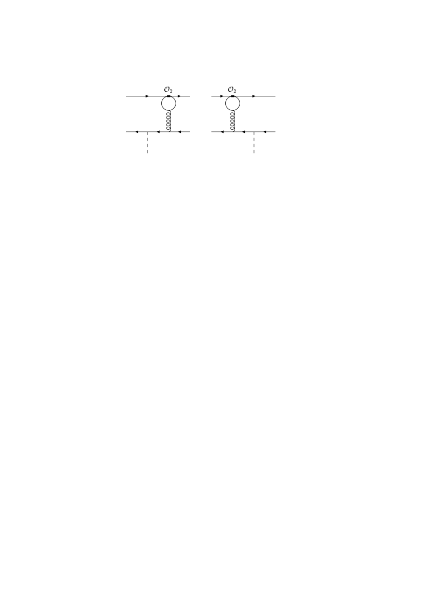
Figure 3: Feynman diagrams contributing to the spectator corrections in $B\to V\gamma$ decays involving the ${\cal O}_{2}$ operator. Row $a$: photon emission from the flavour-changing quark line; Row $b$: photon radiation off the spectator quark line.

The hard-scattering amplitude corresponding to the two diagrams in Fig. 3$a$ involving the emission of the photon from the $b$- or $d$-quarks is as follows:

$${\cal T}^{(3a)}_{ijkl} = \frac{G_{F}}{\sqrt{2}}\,\frac{e}{24\pi^{2}}\,\sum_{f=u,c}V_{fd}^{*}V_{fb}\,C_{2}^{(f)}(\mu)\,\Delta F_{1}\big{(}z^{(f)}_{1}\big{)}\,[\gamma_{\nu}]_{kl}\,$$

$$\times \left[\left\{\gamma_{\nu}-\frac{(k_{2}-l)_{\nu}(k\hskip-4.49997pt/_{2}-l\hskip-4.49997pt/)}{(k_{2}-l)^{2}}\right\}(1-\gamma_{5})\frac{k\hskip-4.49997pt/_{1}+k\hskip-4.49997pt/_{2}-l\hskip-4.49997pt/+m_{b}}{(k_{1}+k_{2}-l)^{2}-m_{b}^{2}}\,e\hskip-4.49997pt/^{*}\right.$$

$$+ \left.e\hskip-4.49997pt/^{*}\,\frac{p\hskip-4.49997pt/_{b}+l\hskip-4.49997pt/-k\hskip-4.49997pt/_{2}}{(p_{b}+l-k_{2})^{2}}\,\left\{\gamma_{\nu}-\frac{(k_{2}-l)_{\nu}(k\hskip-4.49997pt/_{2}-l\hskip-4.49997pt/)}{(k_{2}-l)^{2}}\right\}(1-\gamma_{5})\right]_{ij},$$

where the function $\Delta F_{1}(z^{(f)})$ results from performing the integration over the momentum of the internal quark $f$ having the mass $m_{f}$ [34]:

$$\Delta F_{1}(z)=-\frac{2}{9}-\frac{4}{3}\,\frac{Q_{0}(z)}{z}-\frac{2}{3}\,Q_{0}(z),$$ (3.5)

and its argument is $z^{(f)}_{1}=(k_{2}-l)^{2}/m_{f}^{2}\simeq-Ml_{+}\bar{u}/m_{f}^{2}$, in the limit of the large recoil and to leading order in the inverse $B$-meson mass. In Eq. (3.5) the function $Q_{0}(z)$ is defined as follows:

$$Q_{0}(z)=\int\limits_{0}^{1}du\,\ln\left[1-zu(1-u)\right],$$ (3.6)

and for the case ${\rm Im}\,z>0$ it has the form [34]:

$$Q_{0}(z) = -2-\left[u_{+}(z)-u_{-}(z)\right]\left(\ln\frac{u_{-}(z)}{u_{+}(z)}+i\pi\right),$$ (3.7)

$$u_{\pm}(z) = \frac{1}{2}\left(1\pm\sqrt{1-\frac{4}{z}}\right).$$

The argument $z_{1}^{(f)}$ of the function  $\Delta F_{1}(z_{1}^{(f)})$ in Eq. (3) can be large ($z_{1}^{(u)}\sim M\Lambda_{\rm QCD}/m_{u}^{2}$ for the $u$-quark), and the asymptotic form of this function at large values of its argument is of interest:

$$\Delta F_{1}(z)\bigg{|}_{z\to\infty}\simeq\frac{2}{3}\left[\left(1-\frac{6}{z^{2}}\right)\,\left[\ln\frac{1}{z}+i\pi\right]+\frac{5}{3}+\frac{6}{z}+\frac{3}{z^{2}}\right].$$ (3.8)

Thus, in the case of the internal $u$-quark loop, the function $\Delta F_{1}(z)$ is enhanced by the large logarithm $\ln(m_{u}/M)$. However, as it has been shown in Ref. [35], summing up to all orders in $\alpha_{s}$, the penguin-like diagrams relevant for the $b\to d\gamma$ process can be safely calculated by taking the massless limit for the $u$-quark in the penguin loop. This implies that, despite the superficial appearance, no large enhancement in the amplitude due to $\ln(m_{u}/M)$ is encountered.

Diagrams in Fig. 3$b$ describing the emission of the photon from the spectator quark line yield:

$${\cal T}^{(3b)}_{ijkl} = -\frac{G_{F}}{\sqrt{2}}\,\frac{eQ_{d(u)}}{8\pi^{2}}\,\sum_{f=u,c}V_{fd}^{*}V_{fb}\,C_{2}^{(f)}(\mu)\,\Delta F_{1}\big{(}z^{(f)}_{0}\big{)}$$

$$\times \left[e\hskip-4.49997pt/^{*}\,\frac{k\hskip-4.49997pt/_{1}+k\hskip-4.49997pt/_{2}-p\hskip-4.49997pt/_{b}}{(k_{1}+k_{2}-p_{b})^{2}}\,\gamma_{\nu}+\gamma_{\nu}\,\frac{p\hskip-4.49997pt/_{b}+l\hskip-4.49997pt/-k\hskip-4.49997pt/_{1}}{(p_{b}+l-k_{1})^{2}}\,e\hskip-4.49997pt/^{*}\right]_{kl}$$

$$\times \left[\left\{\gamma_{\nu}-\frac{(p_{b}-k_{1})_{\nu}}{(p_{b}-k_{1})^{2}}\,(p\hskip-4.49997pt/_{b}-k\hskip-4.49997pt/_{1})\right\}(1-\gamma_{5})\right]_{ij},$$

where the argument of the function $\Delta F_{1}(z^{(f)}_{0})$ is $z^{(f)}_{0}=(p_{b}-k_{1})^{2}/m_{f}^{2}\simeq M^{2}\bar{u}/m_{f}^{2}$ in the large recoil limit.

There exists another topological class of diagrams contributing to the spectator corrections involving the effective $bdg^{*}\gamma$ vertex presented in Fig. 4.

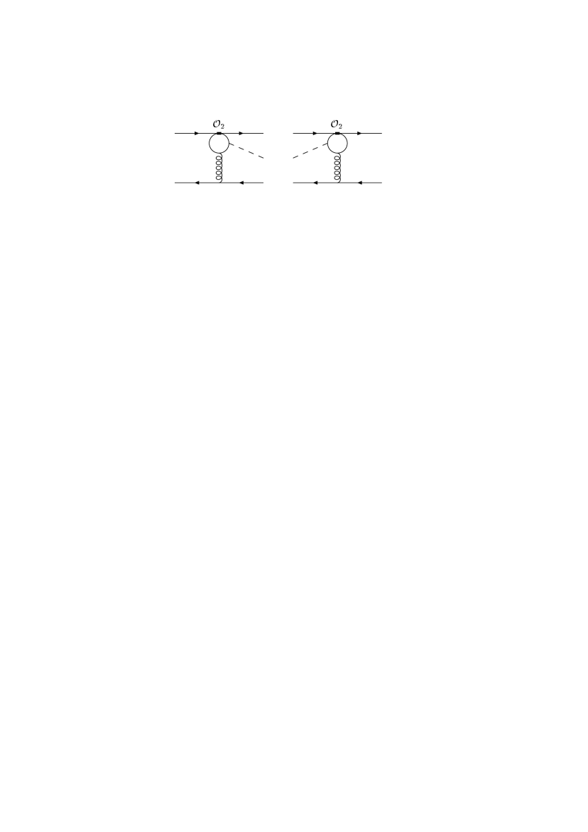
Figure 4: Feynman diagrams contributing to the spectator corrections in $B\to V\gamma$ decays involving the ${\cal O}_{2}$ operator for the case when both the photon and the virtual gluon are emitted from the internal (loop) quark line.

The expression for the one-particle irreducible (OPI) $bdg^{*}\gamma^{*}$ vertex as well as the general $bdg^{*}\gamma^{*}$ case are known since a long time [34]. For an on-shell photon $q^{2}=0$, the OPI vertex is simplified and can be found in Refs. [6] and [7] for the four-dimensional and arbitrary $d$-dimensional momentum spaces, respectively. For the case considered here, the four-dimensional result derived in Ref. [6] is used.

The hard scattering amplitude corresponding to the diagrams shown in Fig. 4 is:

$${\cal T}^{(4)}_{ijkl} = -\frac{G_{F}}{\sqrt{2}}\,\frac{e}{6\pi^{2}}\,\frac{\left[\gamma_{\nu}\right]_{kl}}{(k_{2}-l)^{2}\,(q[k_{2}-l])}\,\sum_{f=u,c}V_{fd}^{*}V_{fb}\,C_{2}^{(f)}(\mu)\,$$

$$\times \left[\left\{\left[q_{\nu}\,{\rm E}(k_{2}-l,e^{*},q)-(q[k_{2}-l])\,{\rm E}(\nu,e^{*},q)\right.\right.\right.$$

$$+ \left.(e^{*}[k_{2}-l])\,{\rm E}(q,\nu,k_{2}-l)-(q[k_{2}-l])\,{\rm E}(e^{*},\nu,k_{2}-l)\right]\Delta i_{5}\big{(}z^{(f)}_{0},z^{(f)}_{1},0\big{)}$$

$$+ \left.\left.\left[(k_{2}-l)^{2}\,{\rm E}(\nu,e^{*},q)+(k_{2}-l)_{\nu}\,{\rm E}(e^{*},k_{2}-l,q)\right]\Delta i_{25}\big{(}z^{(f)}_{0},z^{(f)}_{1},0\big{)}\right\}(1-\gamma_{5})\right]_{ij},$$

where the value $Q_{u}=2/3$ of the electric charge of the quark in the loop is taken into account, and we have used a short-hand notation for the following expression involving products of $\gamma$-matrices:

$${\rm E}(\mu,\nu,\rho)\equiv\frac{1}{2}\,(\gamma_{\mu}\gamma_{\nu}\gamma_{\rho}-\gamma_{\rho}\gamma_{\nu}\gamma_{\mu})=-i\varepsilon_{\mu\nu\rho\sigma}\,\gamma^{\sigma}\,\gamma_{5}.$$ (3.11)

The equality shown above is valid in the four-dimensional space only. In Eq. (3) the functions $\Delta i_{5}(z_{0},z_{1},0)$ and $\Delta i_{25}(z_{0},z_{1},0)$ are [6]:

$$\Delta i_{5}(z_{0},z_{1},0) = -1+\frac{z_{1}}{z_{0}-z_{1}}\,\left[Q_{0}(z_{0})-Q_{0}(z_{1})\right]-\frac{2}{z_{0}-z_{1}}\,\left[Q_{-}(z_{0})-Q_{-}(z_{1})\right],\qquad$$ (3.12)

$$\Delta i_{25}(z_{0},z_{1},0) = Q_{0}(z_{0})-Q_{0}(z_{1}).$$ (3.13)

The auxiliary function $Q_{0}(z)$ is defined in Eq. (3.6), and the other auxiliary function $Q_{-}(z)$ is:

$$Q_{-}(z)=\int\limits_{0}^{1}\frac{du}{u}\,\ln\left[1-zu(1-u)\right],$$ (3.14)

with the explicit form for the case ${\rm Im}\,z>0$ [34]:

$$Q_{-}(z)=\frac{1}{2}\left(\ln\frac{u_{-}(z)}{u_{+}(z)}+i\pi\right)^{2},$$ (3.15)

where the definition of $u_{\pm}(z)$ can be found in Eq. (3.7).

The arguments $z_{0}^{(f)}=(p_{b}-k_{1})^{2}/m_{f}^{2}\simeq M^{2}\bar{u}/m_{f}^{2}$ and $z_{1}^{(f)}=(k_{2}-l)^{2}/m_{f}^{2}\simeq-Ml_{+}\bar{u}/m_{f}^{2}$, already specified above, depend on the internal quark mass $m_{f}$, and in the case of the $u$-quark, they are large practically in all the region of the variables $u$ and $l_{+}$. This is not the case for the $c$-quark contribution in the internal loop, and the charm quark mass-dependent corrections can be important [15, 16]. Note that the value of $z_{1}^{(f)}$ is suppressed by the factor $\Lambda_{\rm QCD}/M$ in comparison with $z_{0}^{(f)}$ and in the framework of the large recoil limit the corrections of order $z_{1}^{(f)}/z_{0}^{(f)}$ can be neglected. In this case, the functions (3.13) and (3.12) are reduced, respectively, to $\Delta i_{25}(z_{0},0,0)=Q_{0}(z_{0})$ and

$$\Delta i_{5}(z_{0},0,0)=-1-\frac{2}{z_{0}}\,Q_{-}(z_{0})=\left\{\begin{array}[]{ll}-1+(4/z_{0})\,\arctan^{2}\left[1/\sqrt{(4/z_{0})-1}\right],&z_{0}<4,\\ -1-\left(\ln\left[u_{-}(z_{0})/u_{+}(z_{0})\right]+i\pi\right)^{2}/z_{0},&z_{0}>4.\end{array}\right.$$ (3.16)

Using the properties of the dilogarithmic function ${\rm Li}_{2}(z)$, the functions $t_{\perp}(u,m_{q})$ in the limit $q^{2}\to 0$ (Eq. (33) derived in Ref. [15]) and $h(u,s)$ (Eq. (35) in Ref. [16]) are the same as the function $\Delta i_{5}(z_{0},0,0)$, derived here, up to overall factors given below:

$$h(\bar{u},s)=-\left.\frac{1}{2}\,t_{\perp}(u,m_{q})\right|_{q^{2}\to 0}=\frac{2}{\bar{u}}\Delta i_{5}(z_{0},0,0).$$

Finally, there are also diagrams where a photon is emitted from the internal quark line due to the effective $b\to s(d)\gamma$ interaction and a gluon is exchanged between the spectator quark and the $b$- or $s(d)$-quarks (see Fig. 5).

Figure 5: Feynman diagrams contributing to the spectator corrections in $B\to V\gamma$ decays involving the ${\cal O}_{2}$ operator for the case when only the photon is emitted from the internal (loop) quark line in the $bs(d)\gamma$ vertex.

Note that in the momentum space the amputated $b\to s(d)\gamma$ vertex due to the four-fermion quark interaction (the ${\cal O}_{2}$ vertex) has the form [34, 7]:

$$I^{(f)}_{\mu}=-\frac{e}{6\pi^{2}}\,\Delta F_{1}\left(\frac{q^{2}}{m_{f}^{2}}\right)\,\left[q_{\mu}q\hskip-4.49997pt/-q^{2}\gamma_{\mu}\right](1-\gamma_{5}),$$ (3.17)

where the function $\Delta F_{1}(z)$ is defined in Eq. (3.5). For the real photon case ($q^{2}=0$), the amplitude contains the scalar product $(e^{*}I^{(f)})\sim(e^{*}q)q\hskip-4.49997pt/-q^{2}e\hskip-4.49997pt/^{*}$ which is zero. This vertex gives a non-vanishing contribution for off-shell photons, such as $b\to s(d)\gamma^{*}\to s(d)l^{+}l^{-}$, which, however, is not the process we are considering in this paper. Hence, for on-shell photon, the Feynman diagrams in Fig. 5 do not contribute to $B\to K^{*}(\rho)\gamma$ (or $b\to s(d)\gamma$).

4 $O(\alpha_{s})$-Corrected Matrix Elements for $B\to V\gamma$
Decays

The convolution of the $B$- and vector ($\rho$- or $K^{*}$-) meson projection operators displayed in (2.8) and (2.9), respectively, with the hard-scattering matrix elements derived in the previous section can be written as:

$$\Delta{\cal M}_{\rm sp}^{(V)}=\frac{G_{F}}{\sqrt{2}}\,\frac{e\alpha_{s}C_{F}}{4\pi N_{c}}\,f_{B}f_{\perp}^{(V)}M\,\left[(e^{*}\varepsilon^{*})+i\,{\rm eps}(e^{*},\varepsilon^{*},n_{-},v)\right]\,\sum_{k=1}^{5}\Delta H^{(V)}_{k},$$ (4.1)

where ${\rm eps}(a,b,c,d)=\varepsilon_{\mu\nu\rho\sigma}a^{\mu}b^{\nu}c^{\rho}d^{\sigma}$ and the upper index $V$ ($=K^{*}$ or $\rho$) characterizes the final vector meson. The dimensionless functions $\Delta H^{(V)}_{k}$ ($k=1,2,3,4,5$) describe the contributions of the sets of Feynman diagrams presented in Figs. 1-5, respectively. In the leading order of the inverse $B$-meson mass ($\sim\Lambda_{\rm QCD}/M$), the result reads as follows:

$$\Delta H^{(V)}_{1}(\mu) \simeq V_{tp}^{*}V_{tb}\,C_{7}^{\rm eff}(\mu)\,m_{b}(\mu)\left[\left<l_{+}^{-1}\right>_{+}\left<\bar{u}^{-1}\right>_{\perp}^{(V)}(\mu)+\left<l_{+}^{-1}\right>_{-}\left<\bar{u}^{-2}\right>_{\perp}^{(V)}(\mu)\right],$$ (4.2)

$$\Delta H^{(V)}_{2}(\mu) \simeq \frac{1}{3}\,V_{tp}^{*}V_{tb}\,C_{8}^{\rm eff}(\mu)\,m_{b}(\mu)\,\left<l_{+}^{-1}\right>_{+}\left<u^{-1}\right>_{\perp}^{(V)}(\mu),$$ (4.3)

$$\Delta H^{(V)}_{3}(\mu) \simeq 0,$$ (4.4)

$$\Delta H^{(V)}_{4}(\mu) \simeq \frac{1}{3}\,C_{2}(\mu)\,M\,\left<l_{+}^{-1}\right>_{+}\left[V_{tp}^{*}V_{tb}\,\left<\bar{u}^{-1}\right>_{\perp}^{(V)}(\mu)+V_{cp}^{*}V_{cb}\,h^{(V)}(z,\mu)\right],$$ (4.5)

$$\Delta H^{(V)}_{5}(\mu) \simeq 0,$$ (4.6)

where $z=m_{c}^{2}/m_{b}^{2}$ and index $p$ in the CKM matrix elements is $p=s$ for the $K^{*}$-meson and $p=d$ for the $\rho$-meson. In the above results we have used the short-hand notation for the integrals over the mesons distribution functions:

$$\left<l_{+}^{N}\right>_{\pm}\equiv\int\limits_{0}^{\infty}dl_{+}\,l_{+}^{N}\,\phi^{(B)}_{\pm}(l_{+}),\qquad\left<f\right>_{\perp,\|}^{(V)}(\mu)\equiv\int\limits_{0}^{1}du\,f(u)\,\phi_{\perp,\|}^{(V)}(u,\mu),$$ (4.7)

and for convenience the following function was introduced:

$$h^{(V)}(z,\mu)=\left<\frac{\Delta i_{5}(z_{0}^{(c)},0,0)+1}{\bar{u}}\right>_{\!\!\perp}^{\!\!(V)}.$$ (4.8)

The function $\Delta H^{(V)}_{2}(\mu)$ [Eq. (4.3)] contains the distribution moment $\left<u^{-1}\right>_{\perp}^{(V)}$, which in the case of the $\rho$-meson can be replaced by $\left<u^{-1}\right>_{\perp}^{(\rho)}\to\left<\bar{u}^{-1}\right>_{\perp}^{(\rho)}$, as the $\rho$-meson distribution function $\phi_{\perp}^{(\rho)}(u)$ is symmetric under the interchange $u\to\bar{u}=1-u$ [32]. This replacement is not valid for the case of the $K^{*}$-meson where a sizable asymmetry under the interchange  $u\to\bar{u}$ is present in the wave-function [32]. The function $\Delta H^{(V)}_{4}(\mu)$ [Eq. (4.5)] arises from the diagrams shown in Fig. 4 with the internal $u$- and $c$-quarks. The contributions of the internal quarks differ by the CKM factor $V_{fp}^{*}V_{fb}$ ($f=u,c$) and the quark masses ($m_{c}$ and $m_{u}$). If the internal quark masses are neglected, an assumption made in the earlier version of this paper but one which we no longer invoke here, then $C_{2}^{(u)}=C_{2}^{(c)}=C_{2}$. This follows as $\Delta H^{(V)}_{4}(\mu)$ originates in the terms $\sim\Delta i_{5}$ from the hard-scattering amplitude ${\cal T}^{(4)}_{ijkl}$, and the replacement $\Delta i_{5}\to-1$ holds in the chiral internal quark limit, $m_{f}=0$. By making use of the unitarity relation $V_{ub}^{*}V_{up}+V_{cb}^{*}V_{cp}+V_{tb}^{*}V_{tp}=0$ their sum can be expressed in terms of one independent CKM combination $V_{tp}^{*}V_{tb}$ (the first term in the bracket of Eq. (4.5)). The correction due to the non-zero $c$-quark mass, which comes weighted by its own CKM factor $V_{cp}^{*}V_{cb}$, is contained in the second term of Eq. (4.5). A detailed discussion of the importance of these corrections will be discussed below. (See, also Ref. [36].)

The result obtained above deserves a number of comments. First, note that the diagrams shown in Fig. 3 involving the operator ${\cal O}_{2}$ do not contribute in the large recoil limit and to leading order in the inverse $B$-meson mass. Second, there are no contributions from the diagrams involving the chromomagnetic operator ${\cal O}_{8}$ for the case where a photon is emitted from the spectator line (Figs. 2$b$). It means that no new contributions to the isospin-breaking corrections to the decay rates $B\to V\gamma$ arise from the hard-spectator corrections in the large recoil limit. Third, the contribution from the diagrams shown in Fig. 1 contains an end-point singularity of the form $\left<\bar{u}^{-2}\right>_{\perp}^{(V)}$ whereas the diagrams in Figs. 2 and 4 give finite contributions. As argued by Beneke and Feldmann in Ref. [12], this end-point singularity describes the soft-gluon physics of the matrix element and can be absorbed into the “soft form factor” $\xi_{\perp}^{(V)}$. This removes the singularity but introduces a factorization scheme (or renormalization convention) for the “soft form factor”. After adopting this procedure, the hard-spectator corrections to the $B\to V\gamma$ decay amplitude depends on the product of the moment of the $B$-meson distribution $\left<l_{+}^{-1}\right>_{+}$ with the vector meson transverse distribution averages: $\left<\bar{u}^{-1}\right>_{\perp}^{(V)}$, $\left<u^{-1}\right>_{\perp}^{(V)}$, and $h^{(V)}=\left<(\Delta i_{5}+1)/\bar{u}\right>_{\perp}^{(V)}$. These products are intrinsically non-perturbative though universal quantities and will have to be determined either by data from elsewhere or else resorting to models for the $B$-meson and the vector meson distribution functions.

It is convenient to introduce the dimensionless quantity [12]

$$\Delta F_{\perp}^{(V)}(\mu)=\frac{8\pi^{2}f_{B}f_{\perp}^{(V)}(\mu)}{N_{c}M\lambda_{B,+}}\left<\bar{u}^{-1}\right>_{\perp}^{(V)}(\mu),$$ (4.9)

where $\lambda_{B,+}^{-1}=\left<l_{+}^{-1}\right>_{+}$ is the first negative moment of the $B$-meson distribution function $\phi_{+}^{(B)}(l_{+})$ which is typically estimated as $\lambda_{B,+}^{-1}=(3\pm 1)$ GeV [33, 12]. At the scale $\mu_{\rm sp}=\sqrt{\mu_{b}\Lambda_{H}}$ of the hard-spectator corrections, and for the central values of the parameters shown in Table 1 with $\lambda_{B,+}^{-1}=3$ GeV, this quantity is evaluated as $\Delta F_{\perp}^{(K^{*})}(\mu_{\rm sp}=1.52~{}{\rm GeV})=1.96$ and $\Delta F_{\perp}^{(\rho)}(\mu_{\rm sp}=1.52~{}{\rm GeV})=1.64$ for the $K^{*}$- and $\rho$-meson, respectively. In term of $\Delta F_{\perp}^{(V)}(\mu)$ the hard-spectator part of $B\to V\gamma$ decay amplitude has the form:

$$\Delta{\cal M}_{\rm sp} = \frac{G_{F}}{\sqrt{2}}\,V_{tp}^{*}V_{tb}\,\frac{\alpha_{s}C_{F}}{4\pi}\,\frac{e}{4\pi^{2}}\,\Delta F_{\perp}^{(V)}(\mu)\left[(pP)\,(e^{*}\varepsilon^{*})+i\,{\rm eps}(e^{*},\varepsilon^{*},p,P)\right]$$

$$\times \left[C_{7}^{\rm eff}(\mu)+\frac{1}{3}\,C_{8}^{\rm eff}(\mu)\,\frac{\left<u^{-1}\right>_{\perp}^{(V)}}{\left<\bar{u}^{-1}\right>_{\perp}^{(V)}}+\frac{1}{3}\,C_{2}(\mu)\left(1+\frac{V_{cp}^{*}V_{cb}}{V_{tp}^{*}V_{tb}}\,\frac{h^{(V)}(z,\mu)}{\left<\bar{u}^{-1}\right>_{\perp}^{(V)}(\mu)}\right)\right]~{},$$

where $P=Mv$ and $p=En_{-}\simeq Mn_{-}/2$ are the four-momenta of the $B$- and vector meson, respectively, and, as in Eqs. (4.2)–(4.6), index $p=s$ or $d$ for the case of $K^{*}$- or $\rho$-meson.

We now proceed to give an analytic result for the function $h^{(V)}(z,\mu)$. To that end we recall that the leading-twist transverse distribution amplitude $\phi_{\perp}^{(V)}(u,\mu)$ of a vector meson is the solution of an evolution equation and has the following general form [32]:

$$\phi_{\perp}^{(V)}(u,\mu)=6u\bar{u}\left[1+\sum_{n=1}^{\infty}a^{(V)}_{\perp n}(\mu)\,C^{3/2}_{n}(u-\bar{u})\right],$$ (4.11)

where $C^{3/2}_{n}(u-\bar{u})$ are the Gegenbauer polynomials [$C^{3/2}_{1}(u-\bar{u})=3(u-\bar{u})$, $C^{3/2}_{2}(u-\bar{u})=3\left[5(u-\bar{u})^{2}-1\right]$/2, etc.] and $a_{\perp n}^{(V)}(\mu)$ are the corresponding Gegenbauer moments (the $\rho$-meson distribution amplitude includes the even moments only). These moments should be evaluated at the scale $\mu$; their scale dependence is governed by [32]:

$$a_{\perp n}^{(V)}(\mu)=\left(\frac{\alpha_{s}(\mu^{2})}{\alpha_{s}(\mu_{0}^{2})}\right)^{\gamma_{n}/\beta_{0}}a_{\perp n}^{(V)}(\mu_{0}),\qquad\gamma_{n}=4C_{F}\left(\sum_{k=1}^{n}\frac{1}{k}-\frac{n}{n+1}\right),$$ (4.12)

where $\beta_{0}=(11N_{c}-2n_{f})/3$ and $\gamma_{n}$ is the one-loop anomalous dimension with $C_{F}=(N_{c}^{2}-1)/(2N_{c})=4/3$. In the limit $\mu\to\infty$ the Gegenbauer moments vanish, $a_{\perp n}^{(V)}(\mu)\to 0$, and the leading-twist transverse distribution amplitude has its asymptotic form:

$$\phi_{\perp}^{(V)}(u,\mu)\to\phi_{\perp}^{({\rm as})}(u)=6u\bar{u}.$$ (4.13)

A simple model of the transverse distribution which includes contributions from the first $a_{\perp 1}^{(V)}(\mu)$ and the second $a_{\perp 2}^{(V)}(\mu)$ Gegenbauer moments only is used here in the analysis. In this approach the quantities $<u^{-1}>_{\perp}^{(V)}$ and $<\bar{u}^{-1}>_{\perp}^{(V)}$ are:

$$<u^{-1}>_{\perp}^{(V)}=3\left[1-a_{\perp 1}^{(V)}(\mu)+a_{\perp 2}^{(V)}(\mu)\right],\qquad<\bar{u}^{-1}>_{\perp}^{(V)}=3\left[1+a_{\perp 1}^{(V)}(\mu)+a_{\perp 2}^{(V)}(\mu)\right],$$ (4.14)

and depend on the scale $\mu$ due to the coefficients $a_{\perp n}^{(V)}(\mu)$. The Gegenbauer moments were evaluated at the scale $\mu_{0}=1$ GeV, yielding [32]: $a_{\perp 1}^{(K^{*})}(1~{}{\rm GeV})=0.20\pm 0.05$ and $a_{\perp 2}^{(K^{*})}(1~{}{\rm GeV})=0.04\pm 0.04$ for the $K^{*}$-meson and $a_{\perp 1}^{(\rho)}(1~{}{\rm GeV})=0$ and $a_{\perp 2}^{(\rho)}(1~{}{\rm GeV})=0.20\pm 0.10$ for the $\rho$-meson. In the same manner, the function $h^{(V)}(z,\mu)$ introduced in Eq. (4.8) can be presented as an expansion on the Gegenbauer moments:

$$h^{(V)}(z,\mu) = h_{0}(z)+a_{\perp 1}^{(V)}(\mu)\,h_{1}(z)+a_{\perp 2}^{(V)}(\mu)\,h_{2}(z)$$

$$= \left[1+3a_{\perp 1}^{(V)}(\mu)+6a_{\perp 2}^{(V)}(\mu)\right]\left<(\Delta i_{5}+1)/\bar{u}\right>^{(0)}_{\perp}$$

$$- 6\left[a_{\perp 1}^{(V)}(\mu)+5a_{\perp 2}^{(V)}(\mu)\right]\left<\Delta i_{5}+1\right>^{(0)}_{\perp}+30\,a_{\perp 2}^{(V)}(\mu)\left<\bar{u}\,(\Delta i_{5}+1)\right>^{(0)}_{\perp},$$

where another short-hand notation is introduced for the integral:

$$\left<f(u)\right>^{(0)}_{\perp}=\int\limits_{0}^{1}du\,f(u)\,\phi_{\perp}^{({\rm as})}(u).$$ (4.16)

Such a decomposition allows us to define the set of functions $h_{n}(z)$ which are dependent on the charm-to-bottom quark mass ratio $z=m_{c}^{2}/m_{b}^{2}$ but are independent of the parameters of the vector meson in consideration. The analytical expressions for the integrals in Eq. (4) are:

$$\left<\frac{\Delta i_{5}(\bar{u}/z,0,0)+1}{\bar{u}}\right>^{\!\!(0)}_{\!\!\perp} = -2z\left\{6-\ln^{3}z+6\,Q_{0}(1/z)\right.$$

$$+ \frac{3i\pi\ln z}{\sqrt{1-4z}}\,[2+Q_{0}(1/z)]-6\,(1-2z)\,Q_{-}(1/z)$$

$$- 6\,[2\ln u_{+}(1/z)-i\pi]\,{\rm Li}_{2}(u_{+}(1/z))$$

$$- 6\,[2\ln u_{-}(1/z)+i\pi]\,{\rm Li}_{2}(u_{-}(1/z))$$

$$+ \left.12\,[{\rm Li}_{3}(u_{+}(1/z))+{\rm Li}_{3}(u_{-}(1/z))]\right\},$$

$$\left<\Delta i_{5}(\bar{u}/z,0,0)+1\right>^{(0)}_{\perp} = \frac{3z}{2}\left(5-12z\right)+9z\left(1-2z\right)Q_{0}(1/z)$$

$$- 6z\left(1-4z+6z^{2}\right)Q_{-}(1/z),$$

$$\left<\bar{u}\,[\Delta i_{5}(\bar{u}/z,0,0)+1]\right>^{(0)}_{\perp} = \frac{z}{18}\,\left(41+144z-720z^{2}\right)$$

$$+ \frac{z}{3}\left(5+34z-120z^{2}\right)Q_{0}(1/z)$$

$$- 2z\left(1-18z^{2}+40z^{3}\right)Q_{-}(1/z),$$

where $Q_{0}(1/z)$ and $Q_{-}(1/z)$ are the functions defined in Eqs. (3.6) and (3.14), respectively, and the dilogarithmic ${\rm Li}_{2}(z)$ and trilogarithmic ${\rm Li}_{3}(z)$ functions have their usual definitions:

$${\rm Li}_{2}(z)=-\int\limits_{0}^{z}\frac{\ln(1-t)}{t}\,dt,\qquad{\rm Li}_{3}(z)=\int\limits_{0}^{z}\frac{{\rm Li}_{2}(t)}{t}\,dt.$$

The result for the charm-quark mass dependent contribution to $\Delta H^{(V)}_{4}$ in Eq. (4.5), $\langle(\Delta i_{5}(z_{0}^{(c)})+1)/\bar{u}\rangle_{\perp}^{(V)}$, derived above in the LEET framework is finite. We concur on this point with the observations made in Refs. [15, 16]. Moreover, we have presented the resulting contribution in an analytic form.

The real and imaginary parts of the functions $h_{n}(z)$ are presented in Figs. 6 (for $n=0$) and 7 (for $n=1$ and $n=2$).

Figure 6: The function $h_{0}(z)$ plotted against the ratio $m_{f}^{2}/m_{b}^{2}$ where $m_{b}$ is the $b$-quark mass. The solid curve is the real part of the function and the dashed curve is its imaginary part.

  

Figure 7: The functions $h_{1}(z)$ (left figure) and $h_{2}(z)$ (right figure) plotted against the ratio $m_{f}^{2}/m_{b}^{2}$ where $m_{b}$ is the $b$-quark mass. The solid curves are the real parts of the functions and the dashed curves are their imaginary parts.

The dependence on $z=m_{c}^{2}/m_{b}^{2}$ of the function $h^{(V)}(z,\mu)$ (4.8) at the mass scale $\mu=\mu_{\rm sp}=1.52$ GeV of hard-spectator corrections is presented in Fig. 8 for the $\rho$- and $K^{*}$-meson.

  

Figure 8: The functions $h^{(\rho)}(z,\mu_{\rm sp})$ for $B\to\rho\gamma$ (left figure) and $h^{(K^{*})}(z,\mu_{\rm sp})$ for $B\to K^{*}\gamma$ (right figure) plotted against the ratio $m_{f}^{2}/m_{b}^{2}$ at the mass scale of hard-spectator corrections $\mu_{\rm sp}=1.52$ GeV. The solid curves are the real parts of the functions and the dashed curves are their imaginary parts.

The values of the corresponding Gegenbauer moments used for evaluations are given in Table 1.

Table 1: Representative values of the $K^{*}$- and $\rho$-meson parameters in the decays $B\to V\gamma$ ($V=\rho,K^{*})$ at the scales $\mu=\mu_{\rm sp}=1.52$ GeV for the hard spectator corrections and $\mu=m_{b,{\rm pole}}=4.65$ GeV for the vertex corrections. The central values of the parameters shown in Tables 4 and 6 are used as inputs with $\sqrt{z}=m_{c}/m_{b}=0.29$.

	$K^{*}$-meson		$\rho$-meson
	$\mu_{\rm sp}$	$m_{b,{\rm pole}}$	$\mu_{\rm sp}$	$m_{b,{\rm pole}}$
$\mu$, [GeV]	1.52	4.65	1.52	4.65
$a_{\perp 1}^{(V)}(\mu)$	0.187	0.164	0	0
$a_{\perp 2}^{(V)}(\mu)$	0.036	0.029	0.179	0.143
$h_{0}(z)$	$3.91+i\,1.64$	$3.91+i\,1.64$	$3.91+i\,1.64$	$3.91+i\,1.64$
$h^{(V)}(z,\mu)$	$4.79+i\,1.46$	$4.68+i\,1.49$	$4.36+i\,1.45$	$4.27+i\,1.48$
$\left<\bar{u}^{-1}\right>_{\perp}^{(V)}(\mu)$	3.67	3.58	3.54	3.43
$h^{(V)}/\left<\bar{u}^{-1}\right>_{\perp}^{(V)}$	$1.31+i\,0.40$	$1.31+i\,0.42$	$1.23+i\,0.41$	$1.25+i\,0.43$
$f_{\perp}^{(V)}(\mu)$, [MeV]	179	167	155	145
$\Delta F_{\perp}^{(V)}(\mu)$	1.96	1.79	1.64	1.48

Comparison of the numerical values for the functions $h_{0}(z)$ and $h^{(V)}(z,\mu_{\rm sp})$ given in this table shows that the influence of the Gegenbauer moments is more sizable in the case of the $K^{*}$-meson, with the real part increasing by $\sim 20\%$ and the imaginary part decreasing by $\sim 10\%$. In the case of the $\rho$-meson, the imaginary part decreases approximately by a similar amount while the real part increases by $\sim 10\%$.

The amplitude (4.1) is proportional to the tensor decay constant $f_{\perp}^{(V)}$ of the vector meson which is a scale dependent parameter. As for the Gegenbauer moments $a_{\perp n}^{(V)}$, its values were defined at the mass scale $\mu_{0}=1$ GeV for the $K^{*}$- and $\rho$-meson following Ref. [32]: $f_{\perp}^{(K^{*})}(1~{}{\rm GeV})=(185\pm 10)$ MeV and $f_{\perp}^{(\rho)}(1~{}{\rm GeV})=(160\pm 10)$ MeV. Their values at an arbitrary scale $\mu$ can be obtained with the help of the evolution equation [32]:

$$f_{\perp}^{(V)}(\mu)=\left(\frac{\alpha_{s}(\mu^{2})}{\alpha_{s}(\mu_{0}^{2})}\right)^{4/(3\beta_{0})}f_{\perp}^{(V)}(\mu_{0}).$$ (4.20)

Central values of the tensor decay constants at the scales $\mu_{\rm sp}=1.52$ GeV and $m_{b,{\rm pole}}=4.65$ GeV are presented in Table 1.

The amplitude (4) allows us to get the hard-spectator corrections to the form factors for the $B\to V$ transitions, with $V=\rho$ or $K^{*}$. The relevant form factors are defined as follows:

$$\left<V(p,\varepsilon^{*})|\bar{Q}\,\sigma^{\mu\nu}q_{\nu}b|\bar{B}(P)\right> = 2T_{1}^{(V)}(q^{2})\,{\rm eps}(\mu,\varepsilon^{*},p,P),$$ (4.21)

$$\left<V(p,\varepsilon^{*})|\bar{Q}\,\sigma^{\mu\nu}\gamma_{5}q_{\nu}b|\bar{B}(P)\right> = -iT_{2}^{(V)}(q^{2})\,[(M^{2}-m_{V}^{2})\,\varepsilon^{*\mu}-(\varepsilon^{*}q)\,(p+P)^{\mu}]\qquad$$

$$-iT_{3}^{(V)}(q^{2})\,(\varepsilon^{*}q)\,\left[q^{\mu}-\frac{q^{2}}{M^{2}-m_{V}^{2}}\,(p+P)^{\mu}\right],$$

where $Q=d$ (for the $\rho$-meson) and $Q=s$ (for the $K^{*}$-meson) are the down quark and strange quark fields. Note that only two form factors $T_{1}^{(V)}(q^{2})$ and $T_{2}^{(V)}(q^{2})$ contribute to the matrix element of the $B\to V\gamma$ decay. Hence, the hard spectator corrections for these form factors from the amplitude (4) for on-shell photon ($q^{2}=0$) are:

$$\Delta_{\rm sp}T_{1}^{(\rho)}(0) = \Delta_{\rm sp}T_{2}^{(\rho)}(0)\simeq\frac{\alpha_{s}C_{F}}{4\pi}\,\frac{\Delta F_{\perp}^{(\rho)}(\mu)}{2}$$

$$\times \left[1+\frac{C_{8}^{(0){\rm eff}}(\mu)}{3C_{7}^{(0){\rm eff}}(\mu)}+\frac{C_{2}^{(0)}(\mu)}{3C_{7}^{(0){\rm eff}}(\mu)}\left(1+\frac{V_{cd}^{*}V_{cb}}{V_{td}^{*}V_{tb}}\,\frac{h^{(\rho)}(z,\mu)}{\left<\bar{u}^{-1}\right>_{\perp}^{(\rho)}(\mu)}\right)\right]~{},$$

for the $\rho$-meson, and

$$\Delta_{\rm sp}T_{1}^{(K^{*})}(0) = \Delta_{\rm sp}T_{2}^{(K^{*})}(0)\simeq\frac{\alpha_{s}C_{F}}{4\pi}\,\frac{\Delta F_{\perp}^{(K^{*})}(\mu)}{2}$$

$$\times \left[1+\frac{C_{8}^{(0){\rm eff}}(\mu)}{3C_{7}^{(0){\rm eff}}(\mu)}\,\frac{\left<u^{-1}\right>_{\perp}^{(K^{*})}(\mu)}{\left<\bar{u}^{-1}\right>_{\perp}^{(K^{*})}(\mu)}+\frac{C_{2}^{(0)}(\mu)}{3C_{7}^{(0){\rm eff}}(\mu)}\left(1-\frac{h^{(K^{*})}(z,\mu)}{\left<\bar{u}^{-1}\right>_{\perp}^{(K^{*})}(\mu)}\right)\right]~{},$$

for the $K^{*}$-meson, in which the asymmetric distribution of the $K^{*}$-meson wave-function is taken into account. In writing the last equation we have used the CKM-unitarity relation $V_{cs}^{*}V_{cb}/V_{ts}^{*}V_{tb}\simeq-1$. We remark that the contribution obtained for the diagrams in Fig. 1 is the same as the one presented in Ref. [12].

5 Branching Ratios for the Decays $B\to K^{*}\gamma$ and
$B\to\rho\gamma$

We shall proceed by first calculating the branching ratios for the decays $B\to K^{*}\gamma$ in the LEET approach. In doing this, we will ignore the isospin-breaking differences between the decay widths $B^{\pm}\to K^{*\pm}\gamma$ and $B^{0}(\bar{B}^{0})\to K^{*0}(\bar{K}^{*0})\gamma$, as they are power suppressed. A recent calculation shows that such isospin-breaking terms can lead to a difference at $(4-8)\%$ level in the amplitudes [37]. Since present data is not precise enough to quantify isospin-violations in the decays $B\to K^{*}\gamma$, and the effect is any case small, we average the data over the charged and neutral decay modes to get a statistically more significant result for the form factor $\xi^{(K^{*})}(0)$ [equivalently $T_{1}^{(K^{*})}(0)$]. As we shall see, the exclusive branching ratios have significant parametric uncertainties, which translate into commensurate theoretical dispersion on the form factors. To reduce some of these uncertainties, we shall also calculate the ratio of the exclusive to inclusive decay widths $R(K^{*}\gamma/X_{s}\gamma)\equiv\Gamma(B\to K^{*}\gamma)/\Gamma(B\to X_{s}\gamma)$, and extract the form factor from the experimentally measured value for $R(K^{*}\gamma/X_{s}\gamma)$.

The branching ratios for the decays $B^{\pm}\to\rho^{\pm}\gamma$ and $B^{0}(\bar{B}^{0})\to\rho^{0}\gamma$ can be related to those of the experimentally measured $B$-decay modes $B^{+}\to K^{*+}\gamma$ and $B^{0}\to K^{*0}\gamma$, using SU(3)-symmetry breaking effects and taking into account other differences in the decay amplitudes of which the differing CKM structure is the most important. An important difference in the $B\to\rho$ and $B\to K^{*}$ transitions is that the annihilation contribution is important in the former, leading to significant isospin violations in the decay rates for $B^{\pm}\to\rho^{\pm}\gamma$ and $B^{0}\to\rho^{0}\gamma$. We shall take these isospin violations in $B\to\rho\gamma$ decays into account. The branching ratios for the $B\to\rho\gamma$ decay modes will be obtained from the expressions

$${\cal B}(B^{\pm}\to\rho^{\pm}\gamma) = \frac{\Gamma_{\rm th}(B^{\pm}\to\rho^{\pm}\gamma)}{\Gamma_{\rm th}(B\to K^{*}\gamma)}\,{\cal B}_{\rm exp}(B^{\pm}\to K^{*\pm}\gamma),$$ (5.1)

$${\cal B}(B^{0}(\bar{B}^{0})\to\rho^{0}\gamma) = \frac{\Gamma_{\rm th}(B^{0}(\bar{B}^{0})\to\rho^{0}\gamma)}{\Gamma_{\rm th}(B\to K^{*}\gamma)}\,{\cal B}_{\rm exp}(B^{0}(\bar{B}^{0})\to K^{*0}(\bar{K}^{*0})\gamma).$$ (5.2)

As we shall see, the theoretical ratios of the branching ratios on the r.h.s. of these equations can be obtained with smaller parametric uncertainties.

5.1 $B\to K^{*}\gamma$ Decays

The present measurements of the branching ratios for $B\to K^{*}\gamma$ decays from the CLEO, BABAR, and BELLE collaborations are summarized in Table 2. They yield the following world averages:

$${\cal B}_{\rm exp}(B^{\pm}\to K^{*\pm}\gamma)=(3.82\pm 0.47)\times 10^{-5},$$ (5.3)

$${\cal B}_{\rm exp}(B^{0}(\bar{B}^{0})\to K^{*0}(\bar{K}^{*0})\gamma)=(4.44\pm 0.35)\times 10^{-5}.$$

Table 2: Experimental branching ratios for the decays $B^{0}(\bar{B}^{0})\to K^{*0}(\bar{K}^{*0})\gamma$ and $B^{\pm}\to K^{*\pm}\gamma$.

Experiment	${\cal B}_{\rm exp}(B^{0}(\bar{B}^{0})\to K^{*0}(\bar{K}^{*0})+\gamma)$	${\cal B}_{\rm exp}(B^{\pm}\to K^{*\pm}+\gamma)$
CLEO [19]	$(4.55^{+0.72}_{-0.68}\pm 0.34)\times 10^{-5}$	$(3.76^{+0.89}_{-0.83}\pm 0.28)\times 10^{-5}$
BELLE [20]	$(4.96\pm 0.67\pm 0.45)\times 10^{-5}$	$(3.89\pm 0.93\pm 0.41)\times 10^{-5}$
BABAR [21]	$(4.23\pm 0.40\pm 0.22)\times 10^{-5}$	$(3.83\pm 0.62\pm 0.22)\times 10^{-5}$

Since we are ignoring the isospin differences in the decay widths of $B\to K^{*}\gamma$ decays, the branching ratios for $B^{\pm}\to K^{*\pm}\gamma$ and $B^{0}(\bar{B}^{0})\to K^{*0}(\bar{K}^{*0})\gamma$ differ essentially by the differing lifetimes of the $B^{\pm}$ and $B^{0}$ mesons. Thus, generically, the branching ratio can be expressed as:

$${\cal B}_{\rm th}(B\to K^{*}\gamma) = \tau_{B}\,\Gamma_{\rm th}(B\to K^{*}\gamma)$$

$$= \tau_{B}\,\frac{G_{F}^{2}\alpha|V_{tb}V_{ts}^{*}|^{2}}{32\pi^{4}}\,m_{b,{\rm pole}}^{2}\,M^{3}\,\left[\xi_{\perp}^{(K^{*})}\right]^{2}\left(1-\frac{m_{K^{*}}^{2}}{M^{2}}\right)^{3}\left|C^{(0){\rm eff}}_{7}+A^{(1)}(\mu)\right|^{2},$$

where $G_{F}$ is the Fermi coupling constant, $\alpha=\alpha(0)=1/137$ is the fine-structure constant, $m_{b,{\rm pole}}$ is the pole $b$-quark mass, $M$ and $m_{K^{*}}$ are the $B$- and $K^{*}$-meson masses, and $\tau_{B}$ is the lifetime of the $B^{0}$- or $B^{+}$-meson which have the following world averages (in picoseconds) [38]:

$$\tau_{B^{0}}=(1.546\pm 0.018)~{}{\rm ps},\qquad\tau_{B^{+}}=(1.647\pm 0.016)~{}{\rm ps}.$$ (5.5)

The product of the CKM-matrix $|V_{tb}V_{ts}^{*}|$ can be estimated from the unitarity fit of the quantity [39]:

$$\left|\frac{V_{tb}V_{ts}^{*}}{V_{cb}}\right|=0.976\pm 0.010~{},$$ (5.6)

and the present measurements of the CKM matrix element $|V_{cb}|=0.0406\pm 0.0019$ [39]. This yields

$$\left|V_{tb}V_{ts}^{*}\right|=0.0396\pm 0.0020~{}.$$ (5.7)

The quantity $\xi_{\perp}^{(K^{*})}$ is the value of the $T_{1}^{(K^{*})}(q^{2})$ form factor in $B\to K^{*}$ transition in Eq. (4.21) and evaluated at $q^{2}=0$ in the HQET limit. For this study, we consider $\xi_{\perp}^{(K^{*})}$ as a free parameter and we will extract its value from the current experimental data on $B\to K^{*}\gamma$ decays. Note that the quantity $\xi_{\perp}^{(K^{*})}$ used here is normalized at the scale $\mu=m_{b,{\rm pole}}$ of the pole $b$-quark mass. The corresponding quantity in Ref. [12] is defined at the scale $\mu=m_{b,{\rm PS}}$ involving the potential-subtracted (PS) $b$-quark mass [40, 41].

The function $A^{(1)}$ in Eq. (5.1) can be decomposed into the following three components:

$$A^{(1)}(\mu)=A_{C_{7}}^{(1)}(\mu)+A_{\rm ver}^{(1)}(\mu)+A_{\rm sp}^{(1)K^{*}}(\mu_{\rm sp})~{}.$$ (5.8)

Here, $A^{(1)}_{C_{7}}$ and $A^{(1)}_{\rm ver}$ are the $O(\alpha_{s})$ (i.e. NLO) corrrections due to the Wilson coefficient $C_{7}^{\rm eff}$ and in the $b\to s\gamma$ vertex, respectively, and $A^{(1)K^{*}}_{\rm sp}$ is the ${\cal O}(\alpha_{s})$ hard-spectator corrections to the $B\to K^{*}\gamma$ amplitude computed in this paper. Their explicit expressions are as follows:

$$A_{C_{7}}^{(1)}(\mu) = \frac{\alpha_{s}(\mu)}{4\pi}\,C^{(1){\rm eff}}_{7}(\mu),$$ (5.9)

$$A_{\rm ver}^{(1)}(\mu) = \frac{\alpha_{s}(\mu)}{4\pi}\left\{\frac{32}{81}\left[13C^{(0)}_{2}(\mu)+27C^{(0){\rm eff}}_{7}(\mu)-9\,C^{(0){\rm eff}}_{8}(\mu)\right]\ln\frac{m_{b}}{\mu}\right.$$

$$- \left.\frac{20}{3}\,C^{(0){\rm eff}}_{7}(\mu)+\frac{4}{27}\left(33-2\pi^{2}+6\pi i\right)C^{(0){\rm eff}}_{8}(\mu)+r_{2}(z)\,C^{(0)}_{2}(\mu)\right\},\qquad$$

$$A_{\rm sp}^{(1)K^{*}}(\mu_{\rm sp}) = \frac{\alpha_{s}(\mu_{\rm sp})}{4\pi}\,\frac{2\Delta F^{(K^{*})}_{\perp}(\mu_{\rm sp})}{9\xi_{\perp}^{(K^{*})}}\left\{3C^{(0){\rm eff}}_{7}(\mu_{\rm sp})\right.$$

$$+ \left.C^{(0){\rm eff}}_{8}(\mu_{\rm sp})\left[1-\frac{6a_{\perp 1}^{(K^{*})}(\mu_{\rm sp})}{\left<\bar{u}^{-1}\right>_{\perp}^{(K^{*})}(\mu_{\rm sp})}\right]+C^{(0)}_{2}(\mu_{\rm sp})\left[1-\frac{h^{(K^{*})}(z,\mu_{\rm sp})}{\left<\bar{u}^{-1}\right>_{\perp}^{(K^{*})}(\mu_{\rm sp})}\right]\right\}.$$

Note, the $O(\alpha_{s})$ corrections arising from the relation between the $\overline{\rm MS}$ mass $\bar{m}_{b}(\mu)$ and the pole mass $m_{b,{\rm pole}}$ in the operator ${\cal O}_{7}$ are included in the vertex corrections. As indicated above, the first two contributions in $A^{(1)}(\mu)$ should be estimated at the scale of the $b$-quark mass $\mu\sim O(m_{b})$, while the hard-spectator correction should be evaluated at the characteristic scale $\mu_{\rm sp}=\sqrt{\mu\Lambda_{\rm H}}$ of the gluon virtuality, where $\Lambda_{\rm H}\simeq 0.5$ GeV is a typical hadronic scale of order $\Lambda_{\rm QCD}$. The functions $r_{2}(z)$, where $z=m_{c}^{2}/m_{b}^{2}$, and the Wilson coefficients in the above equations can be found in Refs. [7, 4]. We recall that the function $h^{(K^{*})}(z)$ from the hard spectator corrections is complex in the region $0<z<1/4$, likewise the function $r_{2}(z)$ from the vertex corrections. The non-asymptotic corrections in the $K^{*}$-meson wave-function $6a_{\perp 1}^{(K^{*})}/\left<\bar{u}^{-1}\right>_{\perp}^{(K^{*})}$ reduce the coefficient of the anomalous chromomagnetic moment $C_{8}^{(0){\rm eff}}(\mu_{\rm sp})$ by about 20%.

We now estimate numerically the importance of the $O(\alpha_{s})$ contributions in the $B\to K^{*}\gamma$ decay amplitude. It is convenient to decompose the vertex correction $A^{(1)}_{\rm ver}(\mu)$ and the hard-spectator correction $A^{(1)K^{*}}_{\rm sp}(\mu)$ into the factorizable $A^{(1)}_{\rm ver,f}(\mu)$ and $A^{(1)K^{*}}_{\rm sp,f}(\mu)$ and non-factorizable $A^{(1)}_{\rm ver,nf}(\mu)$ and $A^{(1)K^{*}}_{\rm sp,nf}(\mu)$ parts. So as not to cause any confusion, our definition is that the first two depend on the effective Wilson coefficient $C^{(0){\rm eff}}_{7}$, and the last two involve the rest of the Wilson coefficients. For the central values of the parameters shown in Table  4, and the indicated values of the the quantities $m_{c}/m_{b}$ and $\mu$, the Wilson coefficient $C^{(0){\rm eff}}_{7}$ in the leading order and the $O(\alpha_{s})$ corrections from Eqs. (5.9)–(5.1) assume the values presented in Table 3.

Table 3: Input parameters and individual contributions in the NLO amplitude for the decay $B\to K^{*}\gamma$ entering in Eqs. (5.1) and (5.8). The entries in the second and third columns refer to the choice of the $b$-quark mass schemes $\overline{\rm MS}$ and the pole mass, respectively. The last two columns correspond to the so-called PS-scheme $b$-quark mass used by Beneke et al. [15], with $m_{c}/m_{b}=0.29$ and $m_{c}/m_{b}=0.22$. Note that the total decay amplitude squared, which is numerically presented in the last row, is truncated to the NLO accuracy.

$m_{c}/m_{b}$	0.29	0.29	0.29	0.22
$\mu$	$\bar{m}_{b}=4.27$ GeV	$m_{b,{\rm pole}}=4.65$ GeV	$m_{b,{\rm PS}}=4.6$ GeV	$m_{b,{\rm PS}}=4.6$ GeV
$C^{(0){\rm eff}}_{7}(\mu)$	$-0.320$	$-0.315$	$-0.318$	$-0.318$
$A^{(1)}_{C_{7}}(\mu)$	$+0.010$	$+0.009$	$+0.010$	$+0.010$
$A^{(1)}_{\rm ver,f}(\mu)$	$+0.032$	$+0.036$	$+0.024$	$+0.024$
$A^{(1)}_{\rm ver,nf}(\mu)$	$-0.076-i\,0.016$	$-0.083-i\,0.016$	$-0.085-i\,0.016$	$-0.103-i\,0.025$
$A^{(1)K^{*}}_{\rm sp,f}(\mu_{\rm sp})$	$-0.038$	$-0.036$	$-0.035$	$-0.035$
$A^{(1)K^{*}}_{\rm sp,nf}(\mu_{\rm sp})$	$-0.016-i\,0.016$	$-0.016-i\,0.015$	$-0.014-i\,0.014$	$-0.008-i\,0.024$
$A^{(1)}(\mu)$	$-0.087-i\,0.032$	$-0.090-i\,0.031$	$-0.100-i\,0.030$	$-0.111-i\,0.049$
$C^{(0){\rm eff}}_{7}+A^{(1)}(\mu)$	$-0.407-i\,0.032$	$-0.405-i\,0.031$	$-0.418-i\,0.030$	$-0.429-i\,0.049$
$|C^{(0){\rm eff}}_{7}+A^{(1)}(\mu)|^{2}$	0.158	0.156	0.165	0.172

What concerns the spectator contributions $A^{(1)K^{*}}_{\rm sp,f}(\mu_{\rm sp})$ and $A^{(1)K^{*}}_{\rm sp,nf}(\mu_{\rm sp})$, the quoted numbers in this table make use of the QCD sum-rules motivated value for the nonperturbative quantity $\xi_{\perp}^{(K^{*})}(0)=0.35$ [15]. The values for the amplitude presented in the second and third columns are obtained for the same pole quark mass ratio $\sqrt{z}=m_{c}/m_{b}=0.29$, but with $\bar{m}_{b}=4.27$ GeV and $m_{b,{\rm pole}}=4.65$ GeV, and calculating the strong coupling $\alpha_{s}(\mu)$ in the two-loop approximation. The last two columns of this table are calculated for comparison with the numerical results by Beneke et al. [15]. They are presented for the two values of the quark mass ratio, $m_{c}/m_{b}=0.29$ (the ratio of the pole masses) and $m_{c}/m_{b}=0.22$ (the ratio of the $\overline{\rm MS}$ $c$-quark mass to the pole $b$-quark mass [18]), but with $m_{b,{\rm PS}}=4.6$ GeV. Note that for the entries in the last two columns the three-loop strong coupling constant $\alpha_{s}$ was used as well as the effect of the non-leading Wilson coefficients and the correction due to the $m_{b,{\rm PS}}$ mass [40, 41] were taken into account in the $A^{(1)K^{*}}_{\rm sp,nf}$ and $A^{(1)}_{\rm ver,f}$ parts of the amplitude, respectively. A comparison of the last-but-one row in this table shows that for the same value of the quark mass ratio $m_{c}/m_{b}$ ($=0.29$), the total amplitude has a negligible dependence on the choice of the $b$-quark mass: $\overline{\rm MS}$, pole, or the PS $b$-quark mass. However, decreasing the ratio $m_{c}/m_{b}$ from 0.29 to 0.22, the amplitude is appreciably enhanced. The dependence of the total decay amplitude squared $|C_{7}^{(0){\rm eff}}(m_{b,{\rm pole}})+A^{(1)}(\bar{m}_{b,{\rm pole}})|^{2}$ (truncated to the $O(\alpha_{s})$ accuracy) on the mass ratio $m_{c}/m_{b}$ is presented in Fig. 9 (left plot). We also draw attention to the marked scale-dependence of the amplitude squared (i.e., of the branching ratio ${\cal B}(B\to K^{*}\gamma$)).

 

Figure 9: The effective coefficient squared in ${\cal B}(B\to K^{*}\gamma)$ appearing in Eq. (5.1) (left figure) and the ratio of the exclusive $B\to K^{*}\gamma$ to the inclusive $B\to X_{s}\gamma$ branching ratios defined in Eq. (5.1) (right figure) plotted against the ratio $m_{c}/m_{b}$ for three values of the scale $\mu$.

It is seen that for $z>0.2$ the amplitude squared becomes sensitive to this mass ratio and falls down fast enough. A similar sensitivity was observed in the inclusive $B\to X_{s}\gamma$ decay rate [18].

Thus, for the central values of the input parameters, we estimate the amplitude squared at the scale of the pole $b$-quark mass as

$$|C_{7}^{(0){\rm eff}}(m_{b,{\rm pole}})+A^{(1)}(m_{b,{\rm pole}})|^{2}\simeq 0.156.$$ (5.12)

In Ref. [15] such a detailed analysis of the amplitude was not shown but the result was presented in the form of the total amplitude squared: $|C_{7}|_{\rm NLO}^{2}=|C^{(0){\rm eff}}_{7}(m_{b,{\rm PS}})+A^{(1)}(m_{b,{\rm PS}})|^{2}=0.175^{+0.029}_{-0.026}$. This value has to be compared with the entries given in the last row (the last two columns) in Table 3 . For the same input parameters, these numbers are somewhat smaller than the ones by Beneke et al [15]. The source of this discrepancy is to be attributed to the fact that we have calculated the branching ratio by keeping only the $O(\alpha_{s})$ corrections in the decay rates, whereas in Ref. [15], the amplitude is corrected to $O(\alpha_{s})$.

To compare our evaluation of the amplitude for $B\to K^{*}\gamma$ decay with the one presented in the paper by Bosch and Buchalla [16], we recall that their calculations were done in the approach where the QCD form factor $T_{1}^{(K^{*})}(0,\mu)$ was used and not its HQET/LEET analog $\xi^{(K^{*})}_{\perp}(0)$. The two form factors are related in $O(\alpha_{s})$ via the relation [12]:

$$T_{1}^{(K^{*})}(0,\bar{m}_{b})=\xi_{\perp}^{(K^{*})}(0)\left(1+\frac{\alpha_{s}(\bar{m}_{b})}{3\pi}\left[\ln\frac{m_{b,{\rm pole}}^{2}}{\bar{m}_{b}^{2}}-1\right]+\frac{\alpha_{s}(\bar{\mu}_{\rm sp})}{6\pi}\frac{\Delta F_{\perp}^{(K^{*})}(\bar{\mu}_{\rm sp})}{\xi_{\perp}^{(K^{*})}(0)}\right)\simeq 1.08\,\xi_{\perp}^{(K^{*})}(0),$$ (5.13)

where $\bar{m}_{b}$ is the $\overline{\rm MS}$ $b$-quark mass and $\bar{\mu}_{\rm sp}=\sqrt{\Lambda_{\rm H}\bar{m}_{b}}\simeq 1.47$ GeV. We also recall that the form factor $T_{1}^{(K^{*})}(0,\mu)$ is a scale-dependent quantity. The $B\to K^{*}\gamma$ decay amplitude includes this from factor in combination with the running $\overline{\rm MS}$ $b$-quark mass $\bar{m}_{b}(\mu)$, and the scale dependence of this product is governed by:

$$\bar{m}_{b}(\mu)\,T_{1}^{(K^{*})}(0,\mu)=\bar{m}_{b}(\bar{m}_{b})\,T_{1}^{(K^{*})}(0,\bar{m}_{b})\left[1+\frac{\alpha_{s}(\mu)}{\pi}\,C_{F}\,\ln\frac{\bar{m}_{b}^{2}}{\mu^{2}}\right].$$ (5.14)

In addition to the form factor and $b$-quark mass, the amplitude also contains the quantity $C_{7}(\mu)=C_{7}^{(0){\rm eff}}(\mu)+A^{(1)}(\mu)$. The transition to the QCD form factor and the use of running $b$-quark mass changes $C_{7}(\mu)$ in a way that all the factorizable $O(\alpha_{s})$ corrections (i.e.,terms proportional to $C_{7}^{(0){\rm eff}}(\mu)$ in $A^{(1)}(\mu)$) are absorbed into $T_{1}^{(K^{*})}(0,\mu)$ and $\bar{m}_{b}(\mu)$. With this interpretation, we give below the numerical estimates of the various contributions to the decay amplitude in $B\to K^{*}\gamma$ calculated by us and compare them with the equivalent quantities in Ref. [16], given in the square brackets. For a meaningful comparison, the values of the input parameters are taken from Ref. [16] with $m_{c}/m_{b}=1.3~{}{\rm GeV}/4.2~{}{\rm GeV}\simeq 0.31$:

$$C^{(0){\rm eff}}_{7}(4.2~{}{\rm GeV})=-0.321\quad[C_{7}^{\rm LO}=-0.322],$$

$$A^{(1)}_{C_{7}}(4.2~{}{\rm GeV})=+0.011\quad[\Delta C_{7}^{\rm NLO}=+0.011],$$

$$A^{(1)}_{\rm ver,nf}(4.2~{}{\rm GeV})=-0.081-i\,0.015\quad[T_{1,8}^{I}=-0.082-i\,0.015],$$ (5.15)

$$A^{(1)K^{*}}_{\rm sp,nf}(1.4~{}{\rm GeV})=-0.014-i\,0.011\quad[T_{1,8}^{II}=-0.014-i\,0.011].$$

$$C^{(0){\rm eff}}_{7}(4.2~{}{\rm GeV})+A^{(1)}(4.2~{}{\rm GeV})=-0.405-i\,0.025\quad[a_{7}(K^{*}\gamma)=-0.407-i\,0.026].$$

We agree with the evaluation of these quantities reported in Ref. [16]. To be precise, we get for the amplitude squared at the $\overline{\rm MS}$ $b$-quark mass scale: $|C_{7}|^{2}_{\rm NLO}=|C^{(0){\rm eff}}_{7}|^{2}+2C^{(0){\rm eff}}_{7}{\rm Re}(A^{(1)})\simeq 0.157$, to be compared with the corresponding value $|C_{7}|^{2}_{\rm NLO}\simeq 0.158$, which can be obtained from Eq. (55) of Ref. [16].

With the numerical estimates given above, and varying the parameters in their stated ranges, we get the following branching ratio for $B\to K^{*}\gamma$ decays:

$${\cal B}_{\rm th}(B\to K^{*}\gamma)\simeq(7.3\pm 1.1)\times 10^{-5}\,\left(\frac{\tau_{B}}{1.6~{}{\rm ps}}\right)\left(\frac{m_{b,{\rm pole}}}{4.65~{}{\rm GeV}}\right)^{2}\left(\frac{\xi_{\perp}^{(K^{*})}}{0.35}\right)^{2}=(7.3\pm 2.7)\times 10^{-5},$$ (5.16)

where the enlarged error in the second equation reflects the assumed error in the nonperturbative quantity, $\xi_{\perp}^{(K^{*})}(0)=0.35\pm 0.07$. This estimate of the branching ratio for $B\to K^{*}\gamma$ is to be compared with the corresponding one from Ref. [15] where a value ${\cal B}_{\rm th}(B\to K^{*}\gamma)=7.9^{+3.5}_{-3.0}\times 10^{-5}$ is obtained. (Note that after some recalculations due to the differences in the definition of the form factor the value $7.1\times 10^{-5}$ obtained for $\tau_{B^{0}}=1.56~{}{\rm ps}$ in Ref. [16] becomes the same as the one in Ref. [15]). If we use instead a value for the $b$-quark pole mass $m_{b,{\rm pole}}=4.8$ GeV, the branching ratio we get is ${\cal B}_{\rm th}(B\to K^{*}\gamma)\simeq(7.8\pm 2.7)\times 10^{-5}$, which is in agreement with the ones presented in Refs. [15, 16]. All these estimates in the LEET approach are larger than the experimental branching ratio for $B\to K^{*}\gamma$, though the attendant theoretical error, estimated as $\pm 40\%$, does not allow to draw a completely quantitative conclusion.

To quantify the price of agreement between the LEET approach and data, we determine the value of the LEET-form factor $\xi_{\perp}^{(K^{*})}(0)$ from the current measurements. To that end, we show the theoretically predicted branching ratios in the NLO accuracy for the decays $B^{0}\to K^{*0}\gamma$ (left figure) and $B^{+}\to K^{*+}\gamma$ (right figure) in Fig. 10 and the corresponding measured branching ratios (horizontal bands), where the solid lines are the central values and the dotted lines define their $\pm 1\sigma$ ranges.

  

Figure 10: Branching ratios for the decays $B^{0}\to K^{*0}\gamma$ (left figure) and $B^{+}\to K^{*+}\gamma$ (right figure) as functions of the LEET form factor $\xi_{\perp}^{(K^{*})}(0)$. Solid lines are the central experimental and theoretically predicted values and the dotted lines delimit the $\pm 1\sigma$ errors in experiment and theory, as discussed in the text.

Theoretical uncertainties on the curves labeled as ${\cal B}_{\rm th}$ are estimated from all the parametric uncertainties, detailed in Table 4 for the decay $B^{0}\to K^{*0}\gamma$, where the last column contains the errors due to the variation of the input parameters resulting from the indicated ranges in the second column. The pole $b$-quark mass is taken from a recent estimate of the same in the NLO accuracy $m_{b,{\rm pole}}=(4.65\pm 0.10)$ GeV [42], and the $B$-meson decay constant in the same accuracy is taken as $f_{B}=(200\pm 20)$ MeV [43, 44]. The enlarged error on the charm-to-bottom quark mass ratio $\sqrt{z}=m_{c}/m_{b}=0.27\pm 0.06$ in Table  4 deserves a comment. We recall from a recent discussion of the inclusive $B\to X_{s}\gamma$ branching ratio in the literature [18] that, within the theoretical accuracy of the present calculations, there exists an intrinsic uncertainty in the interpretation of the quantity $\sqrt{z}$. It has been recently argued in  [18] that the inclusive branching ratio for $B\to X_{s}\gamma$ is uncertain, depending on whether this ratio is interpreted as the one involving the pole masses, $\sqrt{z}=m_{c,{\rm pole}}/m_{b,{\rm pole}}$, or as $\sqrt{z}=\bar{m}_{c}(\mu)/m_{b,{\rm pole}}$ involving the charm quark mass in the $\overline{\rm MS}$ scheme with $m_{c}<\mu<m_{b}$. Typical range for the pole mass interpretation is $\sqrt{z}=0.29\pm 0.02$, while in the latter case the corresponding range is $\sqrt{z}=0.22\pm 0.04$ [18]. This translates into an uncertainty of about 11% in the inclusive decay rate. Not surprisingly, a corresponding sensitivity on $\sqrt{z}$ is also present in the decay rate for the exclusive radiative decays. This has been shown through the $z$-dependence of the matrix element squared for the exclusive decay $B\to K^{*}\gamma$ in Fig. 9 (left plot). To take into account the uncertainty in the decay rate from this source, we use $\sqrt{z}=0.27\pm 0.06$. It is seen from Table 4 that the decay rate for $B\to K^{*}\gamma$ is not sensitive to the variations in the $K^{*0}$-meson wave-function parameters ($f_{\perp}^{(K^{*})}$, $a_{\perp 1}^{(K^{*})}$, and $a_{\perp 2}^{(K^{*})}$) in the indicated ranges, and hence the derived errors on  $\xi_{\perp}^{(K^{*0})}(0)$ from these sources are small. To get the overall theoretical error on $\xi_{\perp}^{(K^{*0})}(0)$, we have added all the individual theoretical errors (given in rows 3 through 11) in quadrature. The errors from the experimental input quantities (first two rows) are given separately.

Table 4: Central values of the parameters and their $\pm 1\sigma$ errors used in estimating the quantity $\xi_{\perp}^{(K^{*})}(0)$ and its error $\delta\xi_{\perp}^{(K^{*})}(0)$ from the branching ratio ${\cal B}_{\rm exp}(B^{0}\to K^{*0}\gamma)$. The parameters in extracting $\xi_{\perp}^{(K^{*})}(0)$ in the $B^{+}\to K^{*+}\gamma$ decay differ essentially in the first two entries, and are discussed in the text.

Parameter	Value	$\delta\xi_{\perp}^{(K^{*0})}(0)$
${\cal B}_{\rm exp}(B^{0}\to K^{*0}\gamma)$	$(4.44\pm 0.35)\times 10^{-5}$	$\pm 0.013$
$\tau_{B^{0}}$	($1.546\pm 0.018$) ps	$\pm 0.002$
$\left|V_{tb}V_{ts}^{*}\right|$	$0.0396\pm 0.0020$	$\pm 0.016$
$m_{b,{\rm pole}}$	($4.65\pm 0.10$) GeV	$\pm 0.006$
$\sqrt{z}=m_{c}/m_{b}$	$0.27\pm 0.06$	${}^{+0.010}_{-0.003}$
$f_{B}$	($200\pm 20$) MeV	$\pm 0.005$
$\lambda_{B,+}^{-1}$	($3\pm 1$) GeV-1	$\pm 0.017$
$f_{\perp}^{(K^{*})}$(1 GeV)	($185\pm 10$) MeV	$\pm 0.003$
$a_{\perp 1}^{(K^{*})}$(1 GeV)	$0.20\pm 0.05$	$\pm 0.002$
$a_{\perp 2}^{(K^{*})}$(1 GeV)	$0.04\pm 0.04$	$\pm 0.001$
$\mu/m_{b,{\rm pole}}$	$0.5-2.0$	$\pm 0.013$
$\xi_{\perp}^{(K^{*0})}(0)$	$0.269\pm 0.028({\rm th})\pm 0.013({\rm exp})$

The form factor $\xi_{\perp}^{(K^{*+})}(0)$ extracted from the $B^{+}\to K^{*+}\gamma$ branching ratio differs somewhat from the one presented in Table 4 due to the difference in the $B^{+}$- and $B^{0}$-meson lifetimes and the corresponding experimental branching ratios. Thus, present data and the NLO expressions in the LEET approach yield the following values for $\xi_{\perp}^{(K^{*})}(0)$:

$$\xi_{\perp}^{(K^{*0})}(0) = 0.27\pm 0.04~{},$$ (5.17)

$$\xi_{\perp}^{(K^{*+})}(0) = 0.24\pm 0.04~{}.$$

The central value of $\xi_{\perp}^{(K^{*0})}(0)$ is marginally larger than $\xi_{\perp}^{(K^{*+})}(0)$ but they are consistent with each other within $1\sigma$. It has been argued recently in Ref. [37] that the small difference may be accounted for by taking into account the isospin-violating contributions from an annihilation contribution in the penguin operator $O_{6}$ in the effective weak Hamiltonian. With improved precision, it may become necessary to include this contribution. As already stated, we have ignored such isospin-violating contributions for the estimates presented for $B\to K^{*}\gamma$ decays in this paper. We also note that the above determination of $\xi_{\perp}^{(K^{*0})}(0)$ and $\xi_{\perp}^{(K^{*+})}(0)$ are in fair agreement with the one presented in Ref. [15], ($\xi_{\perp}^{(K^{*})}(0)=0.24\pm 0.06$).

The non-perturbative parameter $\xi_{\perp}^{(K^{*})}(0)$ can also be extracted from the ratio of the decay rates for the exclusive decay $B\to K^{*}\gamma$ and the inclusive decay $B\to X_{s}\gamma$. In fact, one hopes that some of the parametric uncertainties may be eliminated, or at least reduced, in this ratio. Two particular parameters in point are the quark mass ratio $\sqrt{z}$ and the product of the CKM elements $|V_{tb}V_{ts}^{*}|$. Also, in the experimental measurements some common systematic errors may be eliminated from the ratio. The current world average of the branching ratio for the inclusive $B\to X_{s}\gamma$ decay is [22, 23, 24]:

$${\cal B}_{\rm exp}(B\to X_{s}\gamma)=(3.22\pm 0.40)\times 10^{-4},$$ (5.18)

which yields the following exclusive to inclusive decay width ratio:

$$R_{\rm exp}(K^{*}\gamma/X_{s}\gamma)\equiv\frac{\bar{\cal B}_{\rm exp}(B\to K^{*}\gamma)}{{\cal B}_{\rm exp}(B\to X_{s}\gamma)}=0.13\pm 0.02,$$ (5.19)

where, as for the numerator, we have used an experimental branching ratio averaged over the $B^{\pm}\to K^{*\pm}\gamma$ and $B^{0}(\bar{B}^{0})\to K^{*0}(\bar{K}^{*0})\gamma$ decays: $\bar{\cal B}_{\rm exp}(B\to K^{*}\gamma)=(4.22\pm 0.28)\times 10^{-5}$.

The theoretical expression for the inclusive branching ratio, ${\cal B}_{\rm th}(B\to X_{s}\gamma)$, can be written as [4, 17, 18]:

$${\cal B}_{\rm th}(B\to X_{s}\gamma)=\tau_{B}\,\frac{G_{F}^{2}\alpha m_{b,{\rm pole}}^{5}}{32\pi^{4}}\left|V_{ts}^{*}V_{tb}\right|^{2}\left[\left|C^{(0){\rm eff}}_{7}(\mu)+A^{(1)}_{\rm incl}(\mu)\right|^{2}+B(\mu,\delta)\right],$$ (5.20)

where $\delta$ is a lower cut on the photon energy in the bremsstrahlung corrections, $E_{\gamma,{\rm min}}=(1-\delta)\,m_{b,{\rm pole}}/2$, in the massless limit of the final $s$-quark. The function $A^{(1)}_{\rm incl}$ is the $O(\alpha_{s})$ corrections to the effective $bs\gamma$ vertex while $B(\mu,\delta)$ describe the bremsstrahlung corrections originated by the emission of a real gluon. To get the total branching ratio, we should integrate over all possible photon energies which corresponds to the limit $\delta\to 1$ in Eq. (5.20). In this limit, the vertex and bremsstrahlung corrections are [4, 18, 17]:

$$A^{(1)}_{\rm incl}(\mu) = \frac{\alpha_{s}(\mu)}{4\pi}\left\{C^{(1){\rm eff}}_{7}(\mu)+r_{2}(z)\,C^{(0)}_{2}(\mu)\right.$$

$$- \frac{2}{9}(39+4\pi^{2})\,C^{(0){\rm eff}}_{7}(\mu)+\frac{4}{27}(33-2\pi^{2}+6\pi i)\,C^{(0){\rm eff}}_{8}(\mu)$$

$$+ \left.\frac{32}{81}\left[13C^{(0)}_{2}(\mu)+27C^{(0){\rm eff}}_{7}(\mu)-9C^{(0){\rm eff}}_{8}(\mu)\right]\ln\frac{m_{b}}{\mu}\right\},$$

$$\left.B(\mu,\delta)\right|_{\delta\to 1} = \frac{\alpha_{s}(\mu)}{\pi}\sum_{i\leq j=2,7,8}\left.f_{ij}(\delta)\right|_{\delta\to 1}C_{i}^{(0){\rm eff}}(\mu)C_{j}^{(0){\rm eff}}(\mu),$$ (5.22)

where the explicit forms of the functions $r_{2}(z)$ and $f_{ij}(\delta)$ can be found in Refs. [4, 17, 18]. In the evaluation of the function $f_{88}(\delta)$, which is divergent both in the $s$-quark massless limit and $\delta\to 1$, we take, as advocated in [17], $m_{b}/m_{s}\simeq 50$ and $\delta=0.9$. At NLO, the ratio $R(K^{*}\gamma/X_{s}\gamma)$ can be written as follows:

$$R_{\rm th}(K^{*}\gamma/X_{s}\gamma) = \frac{\bar{\cal B}_{\rm th}(B\to K^{*}\gamma)}{{\cal B}_{\rm th}(B\to X_{s}\gamma)}=\left[\xi_{\perp}^{(K^{*})}\right]^{2}\left[\frac{M}{m_{b,{\rm pole}}}\right]^{3}\left\{1+\frac{\alpha_{s}(\mu)}{\pi}\,\left[1+\frac{4\pi^{2}}{9}\right]\right.\ \qquad$$

$$+ \left.\frac{2\,{\rm Re}\left[A^{(1)K^{*}}_{\rm sp}(\mu_{\rm sp})\right]}{C^{(0){\rm eff}}_{7}(\mu)}-\frac{\alpha_{s}(\mu)}{\pi}\!\!\!\sum_{i\leq j=2,7,8}\!\!\left.f_{ij}(\delta)\right|_{\delta\to 1}\frac{C^{(0)}_{i}(\mu)C^{(0)}_{j}(\mu)}{|C^{(0){\rm eff}}_{7}(\mu)|^{2}}\right\}.$$

The dependencies of this quantity on the charm-to-bottom quark mass ratio $\sqrt{z}$ and on the form factor $\xi_{\perp}^{(K^{*})}(0)$ are presented in Figs. 9 (the right plot) and 11, respectively. It is seen that the ratio $R_{\rm th}(K^{*}\gamma/X_{s}\gamma)$ has a weaker dependence on the ratio $\sqrt{z}$ than the branching ratio for the $B\to K^{*}\gamma$ decay, as this dependence is partially compensated in the last two terms in Eq. (5.1).

Figure 11: The ratio of the exclusive $B\to K^{*}\gamma$ to the inclusive $B\to X_{s}\gamma$ branching ratios, defined in Eq. (5.1), plotted as a function of the LEET form factor $\xi_{\perp}^{(K^{*})}(0)$ and the current experimental measurement of this ratio. The solid lines are the central experimental and theoretically predicted values and the dotted lines delimit the $\pm 1\sigma$ bands.

The numerical analysis allows to estimate the nonperturbative quantity $\xi_{\perp}^{(K^{*})}(0)$ as:

$$\xi_{\perp}^{(K^{*})}(0)=0.24\pm 0.03~{},$$ (5.24)

in which half the error is contributed by experiment. This coincides with the estimate of this quantity from the $B^{+}\to K^{*+}\gamma$ branching ratio presented in Eq. (5.17), where the error is dominated by theory. The average of the three extracted values [Eqs. (5.17) and (5.24)] is:

$$\bar{\xi}_{\perp}^{(K^{*})}(0)=0.25\pm 0.04,\qquad\left[\bar{T}_{1}^{(K^{*})}(0,\bar{m}_{b})=0.27\pm 0.04\right].$$ (5.25)

This estimate is significantly smaller than the corresponding predictions from the QCD sum rules analysis $T_{1}^{(K^{*})}(0)=0.38\pm 0.06$ [26, 25] and from the lattice simulations $T_{1}^{(K^{*})}(0)=0.32^{+0.04}_{-0.02}$ [27]. The reason for this mismatch is not obvious and this point deserves further theoretical study. We shall make some comments in the concluding section.

5.2 $B\to\rho\gamma$ Decays

After comparing the LEET-based approach with experiment in $B\to K^{*}\gamma$ decays, we now present the effect of including the hard-spectator corrections on the branching ratios in $B\to\rho\gamma$ decays and in the isospin-violating ratios and CP-asymmetries in the decay rates.

We recall that ignoring the perturbative QCD corrections to the penguin amplitudes the ratio of the branching ratios for the charged and neutral $B$-meson decays can be written as [10, 2]

$$\frac{{\cal B}(B^{-}\to\rho^{-}\gamma)}{2{\cal B}(B^{0}\to\rho^{0}\gamma)}\simeq\left|1+\epsilon_{A}{\rm e}^{i\phi_{A}}\,\frac{V_{ub}V_{ud}^{*}}{V_{tb}V_{td}^{*}}\right|^{2},$$ (5.26)

where $\epsilon_{A}{\rm e}^{i\phi_{A}}$ includes the dominant $W$-annihilation and possible sub-dominant long-distance contributions. Estimates in the framework of the light-cone QCD sum rules yield typically [8]: $\epsilon_{A}\simeq-0.30\pm 0.07$ and $\epsilon_{A}\simeq 0.03\pm 0.01$ for the decays $B^{-}\to\rho^{-}\gamma$ and $B^{0}\to\rho^{0}\gamma$, respectively, with which a recent calculation also agrees [10]. However, analyses done within the HQET/LEET framework [16, 37] show that the weak annihilation contribution in the $B^{-}\to\rho^{-}\gamma$ has an opposite sign. We have also checked it using the HQET/LEET framework and agree with the positive sign of $\epsilon_{A}$. Taking this into account, we shall use the value $\epsilon_{A}\simeq+0.30\pm 0.07$ in further numerical estimations. The strong interaction phase $\phi_{A}$ disappears in ${\cal O}(\alpha_{s})$ in the chiral limit  [10]. Henceforth we set $\phi_{A}=0$; the isospin-violating correction depends on the unitarity triangle phase $\alpha$ due to the relation:

$$\frac{V_{ub}V_{ud}^{*}}{V_{tb}V_{td}^{*}}=-\left|\frac{V_{ub}V_{ud}^{*}}{V_{tb}V_{td}^{*}}\right|{\rm e}^{i\alpha}=F_{1}+iF_{2}~{}.$$ (5.27)

The next-to-leading order vertex corrections for the branching ratios of the exclusive decays $B^{\pm}\to\rho^{\pm}\gamma$ and $B^{0}\to\rho^{0}\gamma$ can be derived from the corresponding calculations of the inclusive decays $B\to X_{s}\gamma$, discussed in the previous subsection, and $B\to X_{d}\gamma$ [45]. Ignoring the hard-spectator corrections, but including the annihilation contribution, the result was given in Ref. [2]:

$${\cal B}_{\rm th}(B^{\pm}\to\rho^{\pm}\gamma) = \tau_{B^{+}}\,\Gamma_{\rm th}(B^{\pm}\to\rho^{\pm}\gamma)$$

$$= \tau_{B^{+}}\,\frac{G_{F}^{2}\alpha|V_{tb}V_{td}^{*}|^{2}}{32\pi^{4}}\,m_{b,{\rm pole}}^{2}\,M^{3}\,\left(1-\frac{m_{\rho}^{2}}{M^{2}}\right)^{3}\left[\xi_{\perp}^{(\rho)}(0)\right]^{2}\,$$

$$\times \left\{(C^{(0){\rm eff}}_{7}+A^{(1)t}_{R})^{2}+(F_{1}^{2}+F_{2}^{2})\,(A^{u}_{R}+L^{u}_{R})^{2}\right.$$

$$+ \left.2F_{1}\,[C^{(0){\rm eff}}_{7}(A^{u}_{R}+L^{u}_{R})+A^{(1)t}_{R}L^{u}_{R}]\pm 2F_{2}\,[C^{(0){\rm eff}}_{7}A^{u}_{I}-A^{(1)t}_{I}L^{u}_{R}]\right\}~{},$$

where $\xi_{\perp}^{(\rho)}(0)$ is the analogue of the quantity $\xi_{\perp}^{(K^{*})}(0)$, discussed at length in the context of the decays $B\to K^{*}\gamma$, and $L^{u}_{R}=\epsilon_{A}\,C^{(0){\rm eff}}_{7}$. Including the ${\cal O}(\alpha_{s})$ hard-spectator corrections to the matrix elements evaluated at the scale $\mu$, the function $A^{(1)t}$ is modified, and in addition the $u$-quark contribution $A^{u}$ from the penguin can no longer be ignored. We decompose the amplitude $A^{(1)t}(\mu)$ in its three contributing parts:

$$A^{(1)t}(\mu) = A^{(1)}_{C_{7}}(\mu)+A^{(1)}_{\rm ver}(\mu)+A^{(1)\rho}_{\rm sp}(\mu_{\rm sp}),$$ (5.29)

where the functions $A^{(1)}_{C_{7}}(\mu)$ and $A^{(1)}_{\rm ver}(\mu)$ have been defined in Eqs. (5.9) and (5.1), respectively, in the context of the $B\to K^{*}\gamma$ decays. The functions $A^{(1)\rho}_{\rm sp}$ and $A^{u}(\mu)$ are specific to the decays $B\to\rho\gamma$, and both involve hard spectator contributions:

$$A^{(1)\rho}_{\rm sp}(\mu_{\rm sp}) = \frac{\alpha_{s}(\mu_{\rm sp})}{18\pi}\,\frac{\Delta F_{\perp}^{(\rho)}(\mu_{\rm sp})}{\xi_{\perp}^{(\rho)}(0)}\left[3C^{(0){\rm eff}}_{7}(\mu_{\rm sp})+C^{(0){\rm eff}}_{8}(\mu_{\rm sp})+C^{(0)}_{2}(\mu_{\rm sp})\left[1-\frac{h^{(\rho)}(z,\mu_{\rm sp})}{\left<\bar{u}^{-1}\right>^{(\rho)}_{\perp}(\mu_{\rm sp})}\right]\right],$$

$$A^{u}(\mu) = \frac{\alpha_{s}(\mu)}{4\pi}\,C^{(0)}_{2}(\mu)\,\left[r_{2}(z)-r_{2}(0)\right]-\frac{\alpha_{s}(\mu_{\rm sp})}{18\pi}\,C^{(0)}_{2}(\mu_{\rm sp})\,\frac{\Delta F_{\perp}^{(\rho)}(\mu_{\rm sp})}{\xi_{\perp}^{(\rho)}(0)}\,\frac{h^{(\rho)}(z,\mu_{\rm sp})}{\left<\bar{u}^{-1}\right>^{(\rho)}_{\perp}(\mu_{\rm sp})},\qquad$$ (5.30)

The terms proportional to $\Delta F_{\perp}^{(\rho)}(\mu_{\rm sp})$ above are the $O(\alpha_{s})$ hard-spectator corrections which should be evaluated at the typical scale $\mu_{\rm sp}=\sqrt{\mu\Lambda_{\rm H}}$ of the gluon virtuality. The complex function $r_{2}(z)$ of the parameter $z=m_{c}^{2}/m_{b}^{2}$, and the Wilson coefficients in the above equations can be found in Refs. [7, 4]; the function $h^{(\rho)}(z,\mu)$ and the dimensionless quantity $\Delta F_{\perp}^{(\rho)}(\mu)$ are defined through Eqs. (4) and (4.9), respectively. The subscripts $R$ and $I$ in Eq. (5.2) denote the real and imaginary parts of $A^{(1)t}$ and $A^{u}$. The hard-spectator corrections contribute to both the real and imaginary parts of $A^{(1)t}$ and $A^{u}$. They do not depend on the charge of the spectator quark in $B^{0}$- or $B^{\pm}$-mesons, and hence are isospin-conserving. Isospin violations enter mainly via the $W$-annihilation contribution, and they are suppressed in $B^{0}$-meson decays as $L^{u}_{R}(B^{0})\ll L^{u}_{R}(B^{\pm})$.

To simplify the theoretical expressions somewhat, and in view of the smallness of the branching ratios, we would like to present our numerical results in this section in terms of the charge-conjugate averaged branching ratios:

$$\overline{\cal B}_{\rm th}(B^{\pm}\to\rho^{\pm}\gamma) = \frac{1}{2}\left[{\cal B}_{\rm th}(B^{+}\to\rho^{+}\gamma)+{\cal B}_{\rm th}(B^{-}\to\rho^{-}\gamma)\right],$$ (5.31)

$$\overline{\cal B}_{\rm th}(B^{0}\to\rho^{0}\gamma) = \frac{1}{2}\left[{\cal B}_{\rm th}(B^{0}\to\rho^{0}\gamma)+{\cal B}_{\rm th}(\bar{B}^{0}\to\rho^{0}\gamma)\right].$$

Theoretical expressions for these quantities can be easily obtained from the branching ratios (5.2) by neglecting the sign-dependent part. Unless otherwise stated, the results shown below imply an average over the charge-conjugate states.

To illustrate the effect of the NLO corrections on the branching ratios for $B\to\rho\gamma$ decays, we show the relative NLO corrections $\bar{\cal B}_{\rm th}^{\rm NLO}/\bar{\cal B}_{\rm th}^{\rm LO}-1$ to the $B^{\pm}\to\rho^{\pm}\gamma$ and $B^{0}\to\rho^{0}\gamma$ decay rates as functions of the CP phase $\alpha$ in Fig. 12. All other input parameters are fixed to their central values given earlier. What concerns the CKM parameters, we take the ranges for the Wolfenstein parameters from the unitarity fits, yielding [46, 47, 48]:

$$\bar{\rho}=0.20\pm 0.07,\qquad\bar{\eta}=0.39\pm 0.07.$$ (5.32)

They in turn lead to the ranges $|V_{ub}/V_{td}|=0.49\pm 0.09$ and $\alpha$ varying in the range $77^{\circ}\leq\alpha\leq 113^{\circ}$, with $\alpha=93^{\circ}$ as the central value. We will show this range of $\alpha$ by a vertical band in most of the figures presented below. We note from Fig. 12 that the NLO vertex and the hard-spectator corrections are comparable, of order $(30-40)\%$ each, increasing the branching ratio altogether by about $(60-70)\%$ in $B\to\rho\gamma$ decays in the range of $\alpha$ favored by the SM constraints. Note that the total NLO correction for the $B^{0}\to\rho^{0}\gamma$ decays has a very weak dependence on the angle $\alpha$.

  

Figure 12: The relative NLO corrections (in percentage) to the charge-conjugate averaged branching ratios $\bar{\cal B}_{\rm th}(B^{\pm}\to\rho^{\pm}\gamma)$ (left figure) and $\bar{\cal B}_{\rm th}(B^{0}\to\rho^{0}\gamma)$ (right figure) as functions of the unitarity triangle angle $\alpha$ without (dashed curves) and with (solid curves) the hard-spectator corrections. The $\pm 1\sigma$ allowed band of $\alpha$ from the SM unitarity fits is also indicated.

We now proceed to calculate numerically the branching ratios for the decays $B^{\pm}\to\rho^{\pm}\gamma$ and $B^{0}\to\rho^{0}\gamma$ with the help of Eqs. (5.1) and (5.2). The theoretical ratio involving the theoretical decay widths on the r.h.s. of these equations can be written in the form

$$\frac{\overline{\cal B}_{\rm th}(B\to\rho\gamma)}{\overline{\cal B}_{\rm th}(B\to K^{*}\gamma)}=S_{\rho}\left|\frac{V_{td}}{V_{ts}}\right|^{2}\frac{(1-m_{\rho}^{2}/M^{2})^{3}}{(1-m_{K^{*}}^{2}/M^{2})^{3}}\,\zeta^{2}\,\left[1+\Delta R(\rho/K^{*})\right],$$ (5.33)

where $\zeta$ is the ratio of the HQET form factors and $S_{\rho}=1(1/2)$ for $\rho^{\pm}$- ($\rho^{0}$-) meson. In the $SU(3)$-symmetry limit, $\xi_{\perp}^{(\rho)}(0)=\xi_{\perp}^{(K^{*})}(0)$, yielding $\zeta=1$. $SU(3)$-breaking effects in the QCD form factors $T_{1}^{(K^{*})}(0)$ and $T_{1}^{(\rho)}(0)$ have been evaluated within the QCD sum-rules [28]. These can be taken to hold also for the ratio of the HQET form factors. Thus, we take

$$\zeta=\frac{T_{1}^{(\rho)}(0)}{T_{1}^{(K^{*})}(0)}\simeq 0.76\pm 0.06.$$ (5.34)

Taking this and Eq. (5.25) into account, we obtain:

$$\xi_{\perp}^{(\rho)}(0)=0.190\pm 0.034,$$ (5.35)

which can be used in numerical analysis.

The theoretical expression for dynamical function $\Delta R(\rho/K^{*})$ can be written as follows:

$$\Delta R(\rho/K^{*}) = 2\epsilon_{A}\,F_{1}+\epsilon_{A}^{2}(F_{1}^{2}+F_{2}^{2})$$

$$+ \frac{2}{C^{(0){\rm eff}}_{7}}\,{\rm Re}\left[A^{(1)\rho}_{\rm sp}-A^{(1)K^{*}}_{\rm sp}+F_{1}(A^{u}+\epsilon_{A}A^{(1)t})+\epsilon_{A}(F_{1}^{2}+F_{2}^{2})A^{u}\right].$$

Table 5: Central values of the partial amplitudes in $B\to\rho\gamma$ and $B\to K^{*}\gamma$ decays. The column WC $+$ VC is sum of the NLO corrections in the Wilson coefficients (WC) and vertex corrections (VC) which are estimated at the scale $\mu=m_{b,{\rm pole}}=4.65$ GeV; the column HSC contains the hard-spectator contributions evaluated at the scale $\mu_{\rm sp}=1.52$ GeV; and in the last column the total amplitudes (WC+VC+HSC) are presented.

	WC + VC	HSC	total
$A^{(1)t}(\rho\gamma)$	$-0.0428-i\,0.0177$	$-0.0763-i\,0.0274$	$-0.1191-i\,0.0451$
$A^{u}(\rho\gamma)$	$+0.0479+i\,0.0485$	$-0.0708-i\,0.0274$	$-0.0229+i\,0.0211$
$A^{(1)}(K^{*}\gamma)$	$-0.0428-i\,0.0177$	$-0.0711-i\,0.0256$	$-0.1139-i\,0.0433$

For the numerical calculations of $\Delta R(\rho/K^{*})$, we recall that the vertex and the hard-spectator corrections are evaluated at different scales: for the former we use the scale of the $b$-quark mass (pole mass $m_{b,{\rm pole}}=4.65$ GeV in our analysis) and for the last the typical scale is $\mu_{\rm sp}=1.52$ GeV. The combined Wilson coefficient and vertex contributions (WC+VC), the hard-spectator contributions (HSC), and the total contributions (WC+VC+HSC) to the functions $A^{(1)t}(\rho\gamma)$, $A^{(1)}(K^{*}\gamma)$ and $A^{u}(\rho\gamma)$ are presented in Table 5. They correspond to the central values of the input parameters specified earlier. For the assumed input parameters, it is seen that the vertex and hard-spectator contributions (WC$+$VC and HSC) in $A^{(1)t}(\rho\gamma)$ and $A^{(1)}(K^{*}\gamma)$ are of the same sign and comparable to each other. The small difference in the HSC parts is due to $SU(3)$-breaking effects in the ratio of $\Delta F_{\perp}^{(V)}$ [defined in Eq. (4.9)] and $\xi_{\perp}^{(V)}(0)$. For the $\rho$- and $K^{*}$-mesons, their central values are estimated to be:

$$\frac{\Delta F_{\perp}^{(\rho)}(\mu_{\rm sp})}{\xi_{\perp}^{(\rho)}(0)}\simeq 8.61,\qquad\frac{\Delta F_{\perp}^{(K^{*})}(\mu_{\rm sp})}{\xi_{\perp}^{(K^{*})}(0)}\simeq 7.85,$$

where the values of $\xi_{\perp}^{(K^{*})}(0)$, $\xi_{\perp}^{(\rho)}(0)$ and $\Delta F_{\perp}^{(V)}(\mu_{\rm sp})$ are taken from Eqs. (5.25), (5.35) and Table 1, respectively. The main uncertainty ($\sim 30\%$) in these ratios originates from the first negative moment of the $B$-meson $\lambda_{B,+}^{-1}$. The contributions to $A^{u}(\rho\gamma)$ from the vertex and the hard-spectator corrections have opposite signs, and the real part of the sum is rather small. For the numerical estimates, one also needs to know the CKM-functions $F_{1}$ and $F_{2}$ defined by Eq. (5.27). In the analysis the central value resulting from the CKM fits: $\sqrt{F_{1}^{2}+F_{2}^{2}}\simeq|V_{ub}/V_{td}|=0.49$ is used. The dynamical functions $\Delta R(\rho^{\pm}/K^{*\pm})$ and $\Delta R(\rho^{0}/K^{*0})$ for the $B^{\pm}\to\rho^{\pm}\gamma$ and $B^{0}\to\rho^{0}\gamma$ are presented in Fig. 13.

  

Figure 13: The quantities $\Delta R(\rho^{\pm}/K^{*\pm})$ and $\Delta R(\rho^{0}/K^{*0})$ defined in Eq. (5.33) as a function of the unitarity triangle angle $\alpha$ in the leading order (LO) [the dotted lines] and next-to-leading order without (NLO_ver) [dashed lines] and with (NLO_tot) [solid lines] the hard-spectator corrections. The $\pm 1\sigma$ allowed band of $\alpha$ from the SM unitarity fits is also indicated.

It is seen that taking into account the hard-spectator corrections both in the charged and neutral $B$-meson decays makes the branching rates in the leading (LO) [the dotted lines in Fig. 13] and next-to-leading (NLO_tot) [the solid lines in Fig. 13] close to each other. The dependences of the dynamical function $\Delta R(\rho^{\pm}/K^{*\pm})$ on the CKM angle $\alpha$ and on the quark mass ratio $\sqrt{z}=m_{c}/m_{b}$ are presented in Fig. 14. The solid lines correspond to the scale $\mu=m_{b,{\rm pole}}$. It is seen that the dashed lines representing the $\mu=m_{b,{\rm pole}}/2$ and $\mu=2m_{b,{\rm pole}}$ results are very close to each other. Notice also the mild dependence of $\Delta R(\rho^{\pm}/K^{*\pm})$ on the quark mass ratio $\sqrt{z}$.

  

Figure 14: Scale dependence of the quantity $\Delta R(\rho^{\pm}/K^{*\pm})$ defined in Eq. (5.33) as a function of the unitarity triangle angle $\alpha$ (left figure) and the quark mass ratio $\sqrt{z}=m_{c}/m_{b}$ (right figure). The solid curves correspond to the scale $\mu=m_{b,{\rm pole}}$ and the dotted curves delimit the variation in the range $m_{b,{\rm pole}}/2\leq\mu\leq 2m_{b,{\rm pole}}$. The $\pm 1\sigma$ allowed band of $\alpha$ from the SM unitarity fits is also indicated.

The main uncertainties in the dynamical functions come from the uncertainties in the CKM angle $\alpha$ and the nonperturbative parameters $\xi^{(\rho)}_{\perp}(0)$ and $\xi^{(K^{*})}_{\perp}(0)$ which can be seen, in particular, for the $B^{\pm}\to\rho^{\pm}\gamma$ decay from Table 6.

Table 6: Input parameters and the assumed errors used in the evaluation of the function $\Delta R(\rho^{\pm}/K^{*\pm})$, defined in Eq. (5.2). The resulting errors $\delta R(\rho^{\pm}/K^{*\pm})$ are given in the last column. The central value of $\Delta R(\rho^{\pm}/K^{*\pm})$ and the $\pm 1\sigma$ errors obtained by quadrature are given in the last row.

Parameter	Value	$\delta R(\rho^{\pm}/K^{*\pm})$
$\alpha$	$93^{\circ}{}^{+20^{\circ}}_{-16^{\circ}}$	$+0.1612/-0.1321$
$\xi^{(\rho)}_{\perp}(0)$	$0.190\pm 0.035$	$+0.1155/-0.0805$
$\bar{\xi}^{(K^{*})}_{\perp}(0)$	$0.250\pm 0.040$	$+0.0623/-0.0860$
$f_{\perp}^{(\rho)}$(1 GeV)	($160\pm 10$) MeV	$\pm 0.0332$
$a_{\perp 2}^{(\rho)}$(1 GeV)	$0.20\pm 0.10$	$\pm 0.0332$
$\lambda_{B,+}^{-1}$	($3\pm 1$) GeV-1	$\pm 0.0267$
$f_{\perp}^{(K^{*})}$(1 GeV)	($185\pm 10$) MeV	$\pm 0.0244$
$\epsilon_{A}$	$0.30\pm 0.07$	$+0.0187/-0.0163$
$a_{\perp 1}^{(K^{*})}$(1 GeV)	$0.20\pm 0.05$	$\pm 0.0172$
$\left|V_{ub}/V_{td}\right|=\sqrt{F_{1}^{2}+F_{2}^{2}}$	$0.49\pm 0.09$	$+0.0175/-0.0153$
$a_{\perp 2}^{(K^{*})}$(1 GeV)	$0.04\pm 0.04$	$\pm 0.0106$
$\sqrt{z}=m_{c}/m_{b}$	$0.27\pm 0.06$	$+0.0109/-0.0011$
$f_{B}$	($200\pm 20$) MeV	$\pm 0.0080$
$\mu/m_{b,{\rm pole}}$	$0.5-2.0$	$+0.0055/-0.0036$
$m_{b,{\rm pole}}$	($4.65\pm 0.10$) GeV	$\pm 0.0001$
$\Delta R(\rho^{\pm}/K^{*\pm})$	$0.090\pm 0.202$

The function $\Delta R(\rho^{0}/K^{*0})$ involving the neutral $B$-meson decays can be similarly calculated. The allowed ranges of the two functions are estimated to be:

$$\Delta R(\rho^{\pm}/K^{*\pm})=0.09\pm 0.20~{},\qquad\Delta R(\rho^{0}/K^{*0})=0.04\pm 0.14~{}.$$ (5.37)

The central values of both these functions are close to zero, and they impart an uncertainty $\sim 30\%$ and $\sim 15\%$ to the ratios (5.33) of the $B^{\pm}\to\rho^{\pm}\gamma$ to $B^{\pm}\to K^{*\pm}\gamma$ and $B^{0}\to\rho^{0}\gamma$ to $B^{0}\to K^{*0}\gamma$ branching ratios, respectively. Note also that the function analized is increased with increasing the parameter $\epsilon_{A}$ characretized the weak annihilation contribution. While the recent central value obtained at $\epsilon_{A}=+0.3$ is substantially larger than the one from the previous version of the paper (where $\epsilon_{A}=-0.3$ was used), it remains too small to influence on the branching ratio of $B^{\pm}\to\rho^{\pm}\gamma$ decay. Nevertheless, the uncertainty in this function becomes significantly larger.

The product of the CKM matrix elements $|V_{tb}V_{td}^{*}|$ from Eq. (5.2) can be estimated by using the CKM fits, which gives

$$|V_{tb}V_{td}^{*}|=0.0077\pm 0.0011~{}.$$ (5.38)

Taking into account the value $|V_{tb}V_{ts}^{*}|=0.0396\pm 0.0020$ [Eq. (5.7)], we get:

$$\left|\frac{V_{td}}{V_{ts}}\right|=0.194\pm 0.029~{},$$ (5.39)

which allows to predict the values for the branching ratios for $B\to\rho\gamma$ decays with the help of Eqs. (5.1), (5.2), and (5.33). The branching ratios for $B^{\pm}\to\rho^{\pm}\gamma$ and $B^{0}\to\rho^{0}\gamma$ decays are presented in Fig. 15. The vertical bands in these plots delimit the $\pm 1\sigma$ range for $|V_{td}/V_{ts}|$ given in Eq. (5.39).

  

Figure 15: Branching ratios ${\cal B}(B^{\pm}\to\rho^{\pm}\gamma)$ (left figure) and ${\cal}(B^{0}\to\rho^{0}\gamma)$ (right figure) in the NLO-LEET approach as functions of the CKM matrix element ratio $|V_{td}/V_{ts}|$. The solid curves represent the central values and the dashed curves delimit the theoretical $\pm 1\sigma$ variations; the vertical bands show the SM favoured range: $|V_{td}/V_{ts}|=0.194\pm 0.029$.

Due to the present analysis, the $B\to\rho\gamma$ branching ratios can be estimated as

$$\bar{\cal B}_{\rm th}(B^{\pm}\to\rho^{\pm}\gamma)=(0.91\pm 0.33[{\rm th}]\pm 0.11[{\rm exp}])\times 10^{-6},$$ (5.40)

$$\bar{\cal B}_{\rm th}(\bar{B}^{0}\to\rho^{0}\gamma)=(0.50\pm 0.18[{\rm th}]\pm 0.04[{\rm exp}])\times 10^{-6},$$

where the SM favoured range $77^{\circ}\leq\alpha\leq 113^{\circ}$ [46, 47, 48] was used. In the above estimates, the first error is defined by the uncertainties of the theory and the second is from the direct experimental data on the $B\to K^{*}\gamma$ branching ratios (5.3).

These estimates can be compared with the ones obtained in the QCD sum rule approach of Ref. [8]: ${\cal B}(B^{\pm}\to\rho^{\pm}\gamma)=(1.9\pm 1.6)\times 10^{-6}$ and ${\cal B}(B^{0}\to\rho^{0}\gamma)=(0.85\pm 0.65)\times 10^{-6}$, in which only the leading order QCD corrections in $\alpha_{s}$ and annihilation contributions were taken into account. The central values of the estimates presented here are typically a half of the corresponding values in Ref. [8], and the errors in our case are significantly smaller. As shown in Eq. (5.37), the theoretical improvement discussed in the present paper has only a marginal impact on the ratio $R(\rho\gamma/K^{*}\gamma)$, used here and in Ref. [8]. The source of the larger values in Ref. [8] is to be traced back to the differences in the input values of the CKM parameters and the experimental branching ratios for $B\to K^{*}\gamma$ in the two calculations. Present measurements have decreased the allowed range of the ratio $|V_{td}/V_{ts}|$, compared to what was assumed in Ref. [8]. Moreover, the branching ratios ${\cal B}(B\to K^{*}\gamma)$ are now more precisely measured and are found to be smaller than the experimental values en vogue in 1995. These two circumstances, in turn, reduce the central values of the branching ratios ${\cal B}(B^{\pm}\to\rho^{\pm}\gamma)$ and ${\cal B}(B^{0}\to\rho^{0}\gamma)$, and the residual uncertainty is also reduced. We also wish to point out that the estimate of the $B^{-}\to\rho^{-}\gamma$ decay rate presented in Ref. [16] allows a substantially larger uncertainty: ${\cal B}(B^{-}\to\rho^{-}\gamma)=(1.2-3.6)\times 10^{-6}$, reflecting the larger parametric uncertainties in the branching ratio, as well as the fact that the NLO corrections increase the individual branching ratios by typically 60%. As shown in Eq. (5.37), these corrections largely cancel in the ratio. Hence, our predictions for ${\cal B}(B\to\rho\gamma)$ are typically half as large as the ones given in [16]. Finally, compared to the present experimental bounds (at 90%C.L.) [49]: ${\cal B}(B^{\pm}\to\rho^{\pm}\gamma)<0.99\times 10^{-5}$ and ${\cal B}(B^{0}\to\rho^{0}\gamma)<1.06\times 10^{-5}$, one needs to cover an order of magnitude to reach the SM sensitivity in these decays. This should be possible at the present B factories.

6 Isospin-violating Ratios and CP-violating
Asymmetries in $B\to\rho\gamma$ Decays

We now compute the isospin-violating ratios:

$$\Delta^{\pm 0}=\frac{\Gamma(B^{\pm}\to\rho^{\pm}\gamma)}{2\Gamma(B^{0}(\bar{B}^{0})\to\rho^{0}\gamma)}-1~{}.$$ (6.1)

These ratios deviate from zero (the isospin symmetry limit) due to the interference of the short distance penguin amplitudes and long distance tree amplitudes, where the latter are given by the lowest order annihilation contributions, as the ${\cal O}(\alpha_{s})$-contribution to the annihilation amplitude vanishes in the chiral limit in the leading-twist approximation [10]. We present our numerical analysis for the charge-conjugate averaged ratio:

$$\Delta=\frac{1}{2}\,\left[\Delta^{+0}+\Delta^{-0}\right],$$ (6.2)

which is expressed in the NLO perturbative QCD as [2]:

$$\Delta_{\rm LO} \simeq 2\epsilon_{A}\left[F_{1}+\frac{1}{2}\,\epsilon_{A}\,(F_{1}^{2}+F_{2}^{2})\right],$$ (6.3)

$$\Delta_{\rm NLO} \simeq \Delta_{\rm LO}-\frac{2\epsilon_{A}}{C^{(0){\rm eff}}_{7}}\left[F_{1}A^{(1)t}_{R}+(F_{1}^{2}-F_{2}^{2})A^{u}_{R}+\epsilon_{A}(F_{1}^{2}+F_{2}^{2})(A^{(1)t}_{R}+F_{1}A^{u}_{R})\right],\qquad$$ (6.4)

where $\Delta_{\rm LO}$ is the leading-order charge-conjugate averaged ratio. The NLO quantity  $\Delta_{\rm NLO}$ is sensitive to the hard-spectator corrections which are contained in the ${\cal O}(\alpha_{s})$ functions $A^{(1)t}_{R}$ (5.29) and $A^{u}_{R}$ (5.30).

The ratio $\Delta$ is shown as a function of the inner angle $\alpha$ in Fig. 16. The solid curve shows the complete ${\cal O}(\alpha_{s})$-corrected ratio including the vertex and hard spectator corrections, calculated using Eq. (6.4), the dashed curve shows this ratio when only the vertex corrections are included, and the dotted curve shows the lowest order result, obtained using Eq. (6.3).

Figure 16: The charge-conjugate averaged ratio $\Delta$ for $B\to\rho\gamma$ decays defined in Eq. (6.1) as a function of the unitarity triangle angle $\alpha$ in the leading order (dotted curve), next-to-leading order without (dashed curve) and with (solid curve) hard-spectator corrections. The $\pm 1\sigma$ allowed band of $\alpha$ from the SM unitarity fits is also indicated.

We note that taking into account the spectator corrections slightly modifies the ${\cal O}(\alpha_{s})$ vertex-corrected result, obtained in Ref. [2]. Thus, even if one takes a generous error on this quantity, the theoretical precision of $\Delta_{\rm NLO}$ is not perceptibly influenced by the uncertainty in $\Delta F_{\perp}^{(\rho)}$ entering in the hard spectator correction. We also note that the region of $\alpha$ where the NLO corrections are large is not favored by the CKM unitarity constraints in the SM, which yield typically $77^{\circ}\leq\alpha\leq 113^{\circ}$ [46, 47, 48].

In Ref. [16] the charge-conjugate averaged ratio $\Delta$ was found to have an opposite sign than the one obtained in Ref. [2]. Our result presented here, after we have reversed the sign of the annihilation contribution characterized by $\epsilon_{A}$, agrees now with the one given in the former of these references. We would also like to point out that the dependence of $\Delta$ on the inner angle $\alpha$, shown by us in presenting our numerical results, emerges naturally from Eq. (5.27).

Finally, we discuss the direct CP-asymmetry in the $B^{\pm}\to\rho^{\pm}\gamma$ decay rates:

$${\cal A}_{\rm CP}(\rho^{\pm}\gamma)=\frac{{\cal B}(B^{-}\to\rho^{-}\gamma)-{\cal B}(B^{+}\to\rho^{+}\gamma)}{{\cal B}(B^{-}\to\rho^{-}\gamma)+{\cal B}(B^{+}\to\rho^{+}\gamma)}.$$ (6.5)

The CP-asymmetry arises from the interference of the penguin operator ${\cal O}_{7}$ and the four-quark operator ${\cal O}_{2}$ [5, 6]. The expression for the CP-asymmetry in $B^{\pm}\to\rho^{\pm}\gamma$ decays can be written as [2]:

$${\cal A}_{\rm CP}(\rho^{\pm}\gamma)=-\frac{2F_{2}\big{(}A^{u}_{I}-\epsilon_{A}\,A^{(1)t}_{I}\big{)}}{C^{(0){\rm eff}}_{7}\left(1+\Delta_{\rm LO}\right)},$$ (6.6)

where $\Delta_{\rm LO}$ is the charge-conjugate averaged ratio in the leading order (6.3). Note that due to the charm quark mass dependence of the hard-spectator corrections, which enters through the function $h^{(\rho)}(z)$ (4), the functions $A^{(1)t}$ and $A^{u}$ are modified compared to their vertex contributions. More importantly for the CP-asymmetry, the hard spectator contributions are complex. The resulting numerical changes in the functions $A^{u}(\rho\gamma)$ and $A^{(1)t}(\rho\gamma)$, and in their imaginary parts, are illustrated in Table 5.

  

Figure 17: Left figure: Direct CP-asymmetry in the decays $B^{\pm}\to\rho^{\pm}\gamma$ as a function of the unitarity triangle angle $\alpha$ without (dotted curves) and with (solid curves) the hard-spectator corrections. The $\pm 1\sigma$ allowed band of $\alpha$ from the SM unitarity fits is also indicated. Right figure: Direct CP-asymmetry in the decays $B^{\pm}\to\rho^{\pm}\gamma$ as a function of the quark mass ratio $\sqrt{z}=m_{c}/m_{b}$; the scale dependence of the asymmetry is shown in the interval: $m_{b,{\rm pole}}/2\leq\mu\leq 2m_{b,{\rm pole}}$.

The dependence on the angle $\alpha$ of the CP-asymmetry ${\cal A}_{\rm CP}(\rho^{\pm}\gamma)$ is presented in the left plot in Fig. 17. It is seen that the CP-asymmerty is significantly suppressed by the hard-spectator corrections. In the SM favoured interval for $\alpha$, $77^{\circ}\leq\alpha\leq 113^{\circ}$, the direct CP-asymmetry ${\cal A}_{\rm CP}(\rho^{\pm}\gamma)$ takes its maximum value, reaching about $11\%$. The maximum value for the CP-asymmetry without the hard spectator corrections is about $17\%$. Our numerical result for ${\cal A}_{\rm CP}(\rho^{\pm}\gamma)$ agrees now with the corresponding CP-asymmetry calculated in Ref. [16]. The CP-asymmetry shown in the left plot in Fig. 17 is drawn for $\sqrt{z}=m_{c}/m_{b}=0.27$ and $\epsilon_{A}=0.3$. The $z$-dependence of ${\cal A}_{\rm CP}(\rho^{\pm}\gamma)$ is shown in the right plot of Fig. 17; the dependence on the scale $\mu$ of this quantity in the interval $m_{b,{\rm pole}}/2\leq\mu\leq 2m_{b,{\rm pole}}$ is also shown in this figure. The sensitivity of the CP-asymmetry on the quark mass ratio is quite marked. In Fig. 18 we plot the corresponding CP-asymmetry in the decays $B^{0}/\bar{B}^{0}\to\rho^{0}\gamma$, for which the annihilation contribution is both colour and charge suppressed, and setting $\epsilon_{A}=0$ is not a bad approximation.

  

Figure 18: Left figure: Direct CP-asymmetry contribution $a_{\epsilon^{\prime}}$ in ${\cal A}_{\rm CP}(\rho^{0}\gamma)(t)$ in Eq. (6.7) in the decays $B^{0}(\bar{B}^{0})\to\rho^{0}\gamma$ as a function of the unitarity triangle angle $\alpha$ without (dotted curves) and with (solid curves) the hard-spectator corrections. The $\pm 1\sigma$ allowed band of $\alpha$ from the SM unitarity fits is also indicated. Right figure: Direct CP-asymmetry in the decays $B^{0}(\bar{B}^{0})\to\rho^{0}\gamma$ as a function of the quark mass ratio $\sqrt{z}=m_{c}/m_{b}$; the scale dependence of the asymmetry is shown in the interval: $m_{b,{\rm pole}}/2\leq\mu\leq 2m_{b,{\rm pole}}$.

A word of caution in the interpretation of Fig. 18 is in order. We recall that the CP-asymmetry in the decays $B^{0}/\bar{B}^{0}\to\rho^{0}\gamma$ has an additional complication due to the $B^{0}-\bar{B}^{0}$ mixing, which modulates the time-evolution of the CP-asymmetry ${\cal A}_{\rm CP}(\rho^{0}\gamma)$ [50]:

$${\cal A}_{\rm CP}(\rho^{0}\gamma)(t)=a_{\epsilon^{\prime}}\cos(\Delta M_{d}t)+a_{\epsilon+\epsilon^{\prime}}\sin(\Delta M_{d}t)~{},$$ (6.7)

where $\Delta M_{d}\simeq 0.49\,{\rm ps}^{-1}$ is the mass difference between the two mass eigenstates of the $B^{0}-\bar{B}^{0}$ system, and the definitions of the direct $a_{\epsilon^{\prime}}$ and mixing-induced $a_{\epsilon+\epsilon^{\prime}}$ components can be seen in Ref. [50]. The CP-asymmetry shown in Fig. 18 is actually the quantity $a_{\epsilon^{\prime}}$, which is given by Eq. (6.6) with $\epsilon_{A}$ set to zero for the decays $B^{0}(\bar{B}^{0})\to\rho^{0}\gamma$.

To summarize direct CP-asymmetries ${\cal A}_{\rm CP}(\rho^{\pm}\gamma)$ and ${\cal A}_{\rm CP}(\rho^{0}\gamma)$, we remark that the hard spectator corrections decrease the corresponding asymmetries obtained from the vertex contributions alone. The degree of this suppression depends on the annihilation contribution, parametrized here by the quantity $\epsilon_{A}$. In addition to this, the CP-asymmetries depend on both the quark mass ratio $\sqrt{z}$ and the scale $\mu$. Hence, without knowing precisely the values of these quantities, it is difficult to quantify ${\cal A}_{\rm CP}(\rho^{\pm}\gamma)$ and ${\cal A}_{\rm CP}(\rho^{0}\gamma)$. However, in all likelihood, $|{\cal A}_{\rm CP}(\rho^{\pm}\gamma)|$ and $|{\cal A}_{\rm CP}(\rho^{0}\gamma)|$ are less than 10% in the SM.

7 Summary and Concluding Remarks

We summarize our main results and offer some remarks on the underlying theoretical framework. We have computed the hard-spectator corrections in $O(\alpha_{s})$ and leading order in $\Lambda_{\rm QCD}/M$ to the decay widths for $B\to K^{*}\gamma$ and $B\to\rho\gamma$, in the leading-twist approximation, using the Large Energy Effective Theory. This is then combined with the existing contributions from the vertex corrections and the annihilation amplitudes to arrive at the NLO expressions for the corresponding decay rates. The annihilation contributions are important only in the $B\to\rho\gamma$ decays due to the favourable CKM structure. The matrix elements for these decays in $O(\alpha_{s})$, and to leading power in $\Lambda_{\rm QCD}/M$, are finite, also including the intermediate charm quark contributions from the penguin diagrams, correcting an earlier version of this paper, and providing an explicit proof of the factorization Ansatz of Eq. (2.4) advocated by Beneke et al. [11, 12]. For radiative decays $B\to V\gamma$, these proofs have also been provided in the meanwhile in Refs. [16, 15]. We have made extensive comparisons of our derivations and numerical estimates with the ones presented in these papers, pointing out the agreements and some numerical differences related to the hard-spectator corrections. The NLO corrections in the decay rates are substantial, with the branching ratios increasing typically by $60-70\%$ in the NLO approximation. Approximately, a half of this enhancement is due to the vertex corrections, which are common between the corresponding inclusive and exclusive radiative decay rates.

The branching ratios for the decays $B\to K^{*}\gamma$ in the NLO accuracy are then compared with current data to determine the form factor $\xi_{\perp}^{(K^{*})}(0)$ in the LEET approach. For this purpose we have used the measured values of the branching ratios for $B\to K^{*}\gamma$ and $B\to X_{s}\gamma$, getting $\xi_{\perp}^{(K^{*})}(0)=0.25\pm 0.04$, taking into account various parametric uncertainties and experimental errors. Converting it to the form factor in the full QCD, using a relation correct to leading order in $\alpha_{s}$ and $\Lambda_{\rm QCD}/M$ [12], yields $T_{1}^{(K^{*})}(0,\bar{m}_{b})=0.27\pm 0.04$, to be compared with the estimates $T_{1}^{(K^{*})}(0,\bar{m}_{b})=0.38\pm 0.06$ [25, 26], and $T_{1}^{(K^{*})}(0,\bar{m}_{b})=0.32^{+0.04}_{-0.02}$ [27], obtained using the LC-QCD sum rule and Lattice-QCD approaches, respectively. Thus, the form factor in the LEET-based factorization approach, combined with current data, is found to be typically $(15-30)\%$ smaller than the ones in the LC-QCD/Lattice-QCD approaches. Another way to judge the same issue is to use the central value of the form factor $\xi_{\perp}^{(K^{*})}(0)=0.35$ extracted from the LC-QCD sum rules as input and calculate the branching ratio for $B\to K^{*}\gamma$ in the LEET approach. This yields ${\cal B}(B\to K^{*}\gamma)=(7.3\pm 2.7)\times 10^{-5}$, compared to the current experimental value of ${\cal B}_{\rm exp}(B\to K^{*}\gamma)=(4.22\pm 0.28)\times 10^{-5}$, where we have averaged the theory and experiment over the $B^{\pm}$- and $B^{0}/\bar{B}^{0}$-decay modes. Thus, the LEET-based branching ratio is found to be significantly larger than data, though the underlying parametric uncertainties can be used to reduce this difference to some extent [see, Eq. (5.16)]. This discrepancy, while not overwhelming, is discomfortingly large for a precision test of the SM using the exclusive decay rates. Improved data may bridge this gap, bringing in line the LEET-based branching ratios with data, or equivalently the form factors in this approach with the ones in the other two QCD methods. This remains to be seen. Of course, also in the sum rule and lattice approaches to QCD, the desired theoretical accuracy on the form factors is not yet reached. However, despite its tentative nature, the current mismatch between the LEET-based and the other two QCD results in the $B\to V\gamma$ sector may after all turn out to be symptomatic of a generic problem afflicting the LEET approach, having to do with the inadequacy of power corrections in exclusive two-body decays in its present formulation. This, despite the fact that the underlying framework, as formulated in Refs. [11, 15, 16] and also applied in this paper, rests firmly on perturbative QCD factorization, with the argument made even more persuasive by an all order proof of factorization in the strong coupling [51, 52].

What concerns the decay rates in the $B\to\rho\gamma$ decays, we have argued that a more reliable route theoretically is to calculate them via the ratio of the branching ratios ${\cal B}(B\to\rho\gamma)/{\cal B}(B\to K^{*}\gamma)$, defined in Eq. (5.33), using experimental measurement of the $B\to K^{*}\gamma$ decay rates. This ratio depends essentially on the CKM matrix element squared $|V_{td}/V_{ts}|^{2}$, given the non-perturbative quantity $\zeta=\xi_{\perp}^{(\rho)}(0)/\xi_{\perp}^{(K^{*})}(0)$ and a dynamical function called $\Delta R(\rho/K^{*})$, involving the vertex, hard-spectator and annihilation contributions, which is derived and analyzed in this paper. Taking into account various parametric uncertainties, we find that $\Delta R(\rho/K^{*})$ is constrained in the range $|\Delta R(\rho/K^{*})|\leq 0.30$, with the central value around $\Delta R(\rho/K^{*})\simeq 0.09$. This quantifies the statement that the ratio ${\cal B}(B\to\rho\gamma)/{\cal B}(B\to K^{*}\gamma)$ is stable against $O(\alpha_{s})$ and $1/M$-corrections. As shown in this paper, the same does not hold for the individual branching ratios ${\cal B}(B\to\rho\gamma)$ and ${\cal B}(B\to K^{*}\gamma)$. Thus, apart from the dependence on the CKM factor $|V_{td}/V_{ts}|$, whose determination is the principal interest in measuring the ratio ${\cal B}(B\to\rho\gamma)/{\cal B}(B\to K^{*}\gamma)$, the dynamical uncertainties are estimated not to exceed $\pm 20\%$. Using the current branching ratio ${\cal B}_{\rm exp}(B^{\pm}\to K^{*\pm}\gamma)=(3.82\pm 0.47)\times 10^{-5}$, the $SU(3)$-breaking estimate from the LC-QCD sum rule [28], yielding $\zeta=0.76\pm 0.06$, and $\Delta R(\rho/K^{*})$, calculated in this paper, we find ${\cal B}(B^{\pm}\to\rho^{\pm}\gamma)=(0.91\pm 0.44)\times 10^{-6}$, where the present range for the CKM ratio as determined from the unitarity fits, $|V_{td}/V_{ts}|=0.19\pm 0.03$, is folded in the error. The corresponding branching ratio for the neutral $B$-meson decay mode in the same approach is estimated to be: ${\cal B}(B^{0}\to\rho^{0}\gamma)=(0.50\pm 0.22)\times 10^{-6}$. The isospin-violating ratios $\Delta^{\pm 0}$ and its charge-conjugate average $\Delta$ for the decays $B\to\rho\gamma$ are found to be likewise stable against the NLO and $1/M$-corrections, In the expected range of the CKM parameters, we find $|\Delta|\leq 10\%$.

The CP-asymmetries ${\cal A}_{\rm CP}(\rho^{\pm}\gamma)$ and ${\cal A}_{\rm CP}(\rho^{0}\gamma)$ receive contributions from the hard-spectator corrections which tend to decrease their corresponding values estimated from the vertex corrections alone. Unfortunately, the predicted values of the CP-asymmetries are sensitive to both the choice of the scale, as already pointed out in Ref. [16], and the quark mass ratio $\sqrt{z}=m_{c}/m_{b}$. In addition, annihilation contributions play an important role numerically. In line with the QCD sum rule estimates for the magnitude of the annihilation contribution [8, 9], but with the sign in the charged $B$-meson decays as determined in Refs. [16, 37], we have taken $\epsilon_{A}=0.3$ and $\epsilon_{A}\simeq 0$ for the decays $B^{\pm}\to\rho^{\pm}\gamma$ and $B^{0}/\bar{B}^{0}\to\rho^{0}\gamma$, respectively. Typical values for both $|{\cal A}_{\rm CP}(\rho^{\pm}\gamma)|$ and the corresponding direct CP-asymmetry component in $|{\cal A}_{\rm CP}(\rho^{0}\gamma)|$ lie around ($5-10$)%, but the parametric uncertainty in both cases is rather large.

In conclusion, exclusive radiative decays $B\to\rho\gamma$ and $B\to K^{*}\gamma$ (and their semileptonic counterparts) provide an excellent laboratory to test the underlying theory (LEET) and ideas on perturbative non-factorizing corrections put forward by Beneke et al. [11] in the context of $B\to\pi\pi$ and $B\to\pi K$ decays. These latter decays are more involved due to the presence of two strongly interacting particles in the final state and the underlying framework is more tractable in radiative and semileptonic decays. Precise measurements of the radiative and semileptonic decay branching ratios and the related isospin and CP-asymmetries will test this theoretical framework. We have given a fairly detailed phenomenological profile of the radiative decays $B\to K^{*}\gamma$ and $B\to\rho\gamma$ in this paper, and have pointed out some phenomenological issues in this approach related to understanding the current experimental branching ratios for $B\to K^{*}\gamma$ decays, which will have to be resolved on our way to a completely quantitative theory of exclusive radiative decays.

References

-
[1]
N. Cabibbo,
Phys. Rev. Lett. 10, 531 (1963);
M. Kobayashi and T. Maskawa, Prog. Theor. Phys. 49, 652 (1973). - [2] A. Ali, L. T. Handoko and D. London, Phys. Rev. D 63, 014014 (2000) [hep-ph/0006175].
- [3] A. Ali and E. Lunghi, Eur. Phys. J. C 21, 683 (2001) [hep-ph/0105200].
- [4] K. Chetyrkin, M. Misiak and M. Munz, Phys. Lett. B 400, 206 (1997) [Erratum-ibid. B 425, 414 (1997)] [hep-ph/9612313].
- [5] J. M. Soares, Nucl. Phys. B 367, 575 (1991).
- [6] C. Greub, H. Simma and D. Wyler, Nucl. Phys. B 434, 39 (1995) [Erratum-ibid. B 444, 447 (1995)] [hep-ph/9406421].
- [7] C. Greub, T. Hurth and D. Wyler, Phys. Rev. D 54, 3350 (1996) [hep-ph/9603404].
- [8] A. Ali and V. M. Braun, Phys. Lett. B 359, 223 (1995) [hep-ph/9506248].
- [9] A. Khodjamirian, G. Stoll and D. Wyler, Phys. Lett. B 358, 129 (1995) [hep-ph/9506242].
- [10] B. Grinstein and D. Pirjol, Phys. Rev. D 62, 093002 (2000) [hep-ph/0002216].
- [11] M. Beneke, G. Buchalla, M. Neubert and C. T. Sachrajda, Phys. Rev. Lett. 83, 1914 (1999) [hep-ph/9905312].
- [12] M. Beneke and T. Feldmann, Nucl. Phys. B 592, 3 (2001) [hep-ph/0008255].
- [13] M. J. Dugan and B. Grinstein, Phys. Lett. B 255, 583 (1991).
- [14] J. Charles, A. Le Yaouanc, L. Oliver, O. Pene and J. C. Raynal, Phys. Rev. D 60, 014001 (1999) [hep-ph/9812358].
- [15] M. Beneke, T. Feldmann and D. Seidel, Nucl. Phys. B 612, 25 (2001) [hep-ph/0106067].
- [16] S. W. Bosch and G. Buchalla, Nucl. Phys. B 621, 459 (2002) [hep-ph/0106081].
- [17] A. L. Kagan and M. Neubert, Eur. Phys. J. C 7, 5 (1999) [hep-ph/9805303].
- [18] P. Gambino and M. Misiak, Nucl. Phys. B 611, 338 (2001) [hep-ph/0104034].
- [19] S. Chen et al. [CLEO Collaboration], Phys. Rev. Lett. 87, 251807 (2001) [hep-ex/0108032].
- [20] H. Tajima [BELLE Collaboration], Int. J. Mod. Phys. A 17, 2967 (2002) [arXiv:hep-ex/0111037].
- [21] B. Aubert et al. [BABAR Collaboration] Phys. Rev. Lett. 88, 101805 (2002) [hep-ex/0110065]
- [22] D. G. Cassel [CLEO Collaboration], Int. J. Mod. Phys. A 17, 2951 (2002) [arXiv:hep-ex/0111041].
- [23] R. Barate et al. [ALEPH Collaboration], Phys. Lett. B429, 169 (1998).
- [24] K. Abe et al. [BELLE Collaboration], Phys. Lett. B 511, 151 (2001) [hep-ex/0103042].
- [25] P. Ball and V. M. Braun, Phys. Rev. D 58, 094016 (1998) [hep-ph/9805422].
- [26] A. Ali, P. Ball, L. T. Handoko and G. Hiller, Phys. Rev. D 61, 074024 (2000) [hep-ph/9910221].
- [27] L. Del Debbio, J. M. Flynn, L. Lellouch and J. Nieves [UKQCD Collaboration], Phys. Lett. B 416, 392 (1998) [hep-lat/9708008].
- [28] A. Ali, V. M. Braun and H. Simma, Z. Phys. C 63, 437 (1994) [hep-ph/9401277].
- [29] M. Bander, D. Silverman and A. Soni, Phys. Rev. Lett. 44, 7 (1980) [Erratum-ibid. 44, 962 (1980)].
- [30] G. Buchalla, A. J. Buras and M. E. Lautenbacher, Rev. Mod. Phys. 68, 1125 (1996) [hep-ph/9512380].
- [31] J.D. Bjorken and S.D. Drell, Relativistic Quantum Fields (McGraw-Hill, New York, 1965).
- [32] P. Ball, V. M. Braun, Y. Koike and K. Tanaka, Nucl. Phys. B 529, 323 (1998) [hep-ph/9802299].
- [33] A. G. Grozin and M. Neubert, Phys. Rev. D 55, 272 (1997) [hep-ph/9607366].
- [34] H. Simma and D. Wyler, Nucl. Phys. B 344, 283 (1990).
- [35] M. Abud, G. Ricciardi and G. Sterman, Phys. Lett. B 437, 169 (1998) [hep-ph/9712346].
- [36] G. Buchalla, G. Isidori and S. J. Rey, Nucl. Phys. B 511, 594 (1998) [hep-ph/9705253].
- [37] A. L. Kagan and M. Neubert, Phys. Lett. B 539, 227 (2002) [hep-ph/0110078].
- [38] J. Alcaraz et al. (B-Lifetime Working Group), http://www.lephfs.web.cern.ch/LEPHFS/.
- [39] D. E. Groom et al. [Particle Data Group Collaboration], Eur. Phys. J. C 15, 1 (2000).
- [40] M. Beneke, Phys. Lett. B 434, 115 (1998) [hep-ph/9804241].
- [41] M. Beneke and A. Signer, Phys. Lett. B 471, 233 (1999) [hep-ph/9906475].
- [42] J. H. Kühn and M. Steinhauser, Nucl. Phys. B 619, 588 (2001) [hep-ph/0109084].
- [43] A. A. Penin and M. Steinhauser, Phys. Rev. D 65, 054006 (2002) [hep-ph/0108110].
- [44] M. Jamin and B. O. Lange, Phys. Rev. D 65, 056005 (2002) [hep-ph/0108135].
- [45] A. Ali, H. Asatrian and C. Greub, Phys. Lett. B 429, 87 (1998) [hep-ph/9803314].
- [46] A. Hocker, H. Lacker, S. Laplace and F. Le Diberder, Eur. Phys. J. C 21, 225 (2001) [hep-ph/0104062].
- [47] A. Ali and D. London, Eur. Phys. J. C 9, 687 (1999) [hep-ph/9903535].
- [48] A. Ali and E. Lunghi, Eur. Phys. J. C 26, 195 (2002) [arXiv:hep-ph/0206242].
- [49] B. Casey [BELLE Collaboration], contributed talk at the Moriond-QCD conference, March 2001.
- [50] A. Ali, G. Kramer and C. D. Lü, Phys. Rev. D 59, 014005 (1999) [hep-ph/9805403].
- [51] M. Beneke, G. Buchalla, M. Neubert and C. T. Sachrajda, Nucl. Phys. B 591, 313 (2000) [hep-ph/0006124].
- [52] C. W. Bauer, D. Pirjol and I. W. Stewart, Phys. Rev. Lett. 87, 201806 (2001) [hep-ph/0107002].