Abstract

Adjoint supermultiplets (1,3,0) and (8,1,0) modify the evolution of gauge couplings. If the unification of gauge couplings occurs at the string scale, their masses are fixed at around $10^{13}$ GeV. This scale coincides with expected gaugino condensation scale in the hidden sector $M_{string}^{2/3}m^{1/3}_{3/2}\sim 10^{13}$ GeV. We show how neutrino masses arise in this unified model which naturally explain the present atmospheric and solar neutrino data. The out-of-equilibrium decay of the superfield (1,3,0) at $10^{13}$ GeV may also lead to a lepton asymmetry which then gets converted into the present observed baryon asymmetry of the Universe.

It is interesting to study the adjoint SU(2) triplet with no hypercharge $T\equiv(1,3,0)$ having a mass approximately $10^{13}$ GeV. In a supersymmetric theory, the lepton superfield $L_{i}\equiv(\nu_{i},l_{i})$, the Higgs superfield $H_{2}\equiv(h_{2}^{+},h_{2}^{0})$, and the superfield $T\equiv(T^{+},T^{0},T^{-})$ may be connected by the Yukawa coupling $h^{i}_{T}~{}L_{i}~{}H_{2}~{}T$. As $H_{2}$ gets a nonzero vacuum expectation value (VEV) given by $v_{2}\equiv v~{}\sin\beta$, where $\tan\beta\equiv\langle h_{2}^{0}\rangle/\langle h_{1}^{0}\rangle$, the neutrino $\nu$ pairs up with the fermion $T^{0}$ to form a Dirac mass and because $T$ has an allowed Majorana mass $M_{2}$, a seesaw mass is generated for $\nu$: [1]

$$m_{\nu}={h^{2}_{T}~{}v^{2}~{}\sin^{2}~{}\beta\over 2M_{2}},$$ (1)

where the extra factor of 2 comes from the fact that $T^{0}$ couples to $(\nu h_{2}^{0}+lh_{2}^{+})/\sqrt{2}$. The difference between this and the canonical seesaw mechanism [2] is the use of an SU(2) triplet instead of a singlet. This means that whereas the latter has negligible influence on the evolution of gauge couplings, the former changes it in a significant way. It is thus possible to have gauge coupling unification at the string scale [3] with $M_{2}\sim 10^{13}$ GeV as well as a realistic theory of neutrino mass and leptogenesis consistent with present atmospheric and solar neutrino experiments [4, 5], as shown below.

One-loop string effects could lower the tree-level value of the string scale $M_{string}=g_{string}M_{Plank}$ somewhat, and one calculates [6] that the string unification scale is modified to

$$M_{string}=g_{string}\times 5.27\times 10^{17}~{}{\rm GeV}\simeq 5.27\times 10^{17}~{}{\rm GeV}.$$ (2)

Furthermore, string models having a $G\times G$ structure, when broken to the diagonal subgroup, naturally contain adjoint scalars with zero hypercharge. In this paper, we minimally extend the canonical supersymmetric standard model by including the superfields $T\equiv(1,3,0)$, $O\equiv(8,1,0)$ and $S\equiv(1,1,0)$ [7]. We will show that if the unification of gauge couplings occurs at the string scale, two-loop renormalization-group equations (RGE) will fix the masses of $T$ and $O$ at the well-motivated intermediate scale $M_{I}\sim M_{string}^{2/3}m^{1/3}_{3/2}\sim 10^{13}$ GeV, which turns out to be precisely the mass scale $M_{2}$ for $T\equiv(1,3,0)$ in Eq. (1). In our RGE analysis, we consistently include the effects of all Yukawa couplings, among which are the constraints from our present knowledge of the neutrino mass matrix to account for the observed atmospheric and solar neutrino oscillations. (In previous papers [3], this important new possibility was not recognized.)

The dimensionless Yukawa couplings of this model in standard superfield notation is given by

$${\cal L}=h_{\tau}~{}[L~{}H_{1}~{}\overline{E}]+~{}h_{b}~{}[Q~{}H_{1}~{}\overline{D}]+h_{t}~{}[Q~{}H_{2}~{}\overline{U}]+h_{T}~{}[L~{}H_{2}~{}T]+h_{S}~{}[L~{}H_{2}~{}S]+h_{\lambda}~{}[T~{}T~{}S],$$ (3)

where we have introduced a singlet $S\equiv(1,1,0)$, the utility of which will be explained later.

$$\begin{array}[]{|c||c||c|}\hline\cr Superfields&SU(3)_{c}\times SU(2)_{L}\times U(1)_{Y}&Anomalous~{}Dimension\\ \hline\cr L&(1,2,-{1\over 2}\sqrt{3\over 5})&{1\over 16\pi^{2}}~{}[h^{2}_{\tau}+h^{2}_{T}+h^{2}_{S}-{3\over 2}g^{2}_{2}-{3\over 10}g^{2}_{Y}]\\ \overline{E}&(1,1,\sqrt{3\over 5})&{1\over 16\pi^{2}}~{}[2h^{2}_{\tau}-{6\over 5}g^{2}_{Y}]\\ \overline{D}&(\overline{3},1,{1\over 3}\sqrt{3\over 5})&{1\over 16\pi^{2}}~{}[2h^{2}_{b}-{8\over 3}g^{2}_{c}-{4\over 30}g^{2}_{Y}]\\ \overline{U}&(\overline{3},1,-{2\over 3}\sqrt{3\over 5})&{1\over 16\pi^{2}}~{}[2h^{2}_{t}-{8\over 3}g^{2}_{3}-{8\over 15}g^{2}_{Y}]\\ Q&(3,2,{1\over 6}\sqrt{3\over 5})&{1\over 16\pi^{2}}~{}[h^{2}_{t}+h^{2}_{b}-{8\over 3}g^{2}_{3}-{3\over 2}g^{2}_{2}-{1\over 30}g^{2}_{Y}]\\ H_{1}&(1,2,-{1\over 2}\sqrt{3\over 5})&{1\over 16\pi^{2}}~{}[h^{2}_{\tau}+3h^{2}_{b}-{3\over 2}g^{2}_{2}-{3\over 10}g^{2}_{Y}]\\ H_{2}&(1,2,{1\over 2}\sqrt{3\over 5})&{1\over 16\pi^{2}}~{}[3h^{2}_{t}+h^{2}_{T}+h^{2}_{S}-{3\over 2}g^{2}_{2}-{3\over 10}g^{2}_{Y}]\\ \hline\cr T&(1,3,0)&{1\over 16\pi^{2}}~{}[h^{2}_{T}+h^{2}_{\lambda}-{4}g^{2}_{2}]\\ S&(1,1,0)&{1\over 16\pi^{2}}~{}[3~{}h^{2}_{\lambda}+2~{}h^{2}_{S}]\\ O&(8,1,0)&{1\over 16\pi^{2}}~{}[-{6}g^{2}_{3}]\\ \hline\cr\end{array}$$

Table 1: Representations and anomalous dimensions of superfields

At the two-loop level, the evolution of the gauge couplings is governed by the following equation, where we have defined $t=ln~{}\mu/2\pi$.

$${d\alpha_{i}\over dt}={b_{i}}\alpha^{2}_{i}+\sum_{j}{b_{ij}\over 4\pi}\alpha^{2}_{i}\alpha_{j}-\sum_{k}{a_{ik}\over 4\pi}\alpha^{2}_{i}Y_{k},$$ (4)

The one-loop coefficients $b_{i}$ and the two-loop coefficients $b_{ij}$ can be easily derived [7]. Also the effect of the Yukawa couplings on the running of the gauge couplings is brought in by the coefficients $a_{ij}$. They are given by

$$b_{i}=\left(\begin{array}[]{c}\frac{33}{5}\\ 1+2~{}n_{T}\\ -3+3~{}n_{O}\end{array}\right),\,~{}~{}~{}a_{ik}=\left(\begin{array}[]{cccccc}\frac{26}{5}&\frac{14}{5}&\frac{18}{5}&\frac{6}{5}&\frac{6}{5}&0\\ 6&6&2&6&2&4\\ 4&4&0&0&0&0\end{array}\right),$$ (5)

and

$$b_{ij}=\left(\begin{array}[]{ccc}\frac{199}{25}&\frac{27}{5}&\frac{88}{5}\\ \frac{9}{5}&25+24~{}n_{T}&24\\ \frac{11}{5}&9&14+54~{}n_{O}\end{array}\right),$$ (6)

In the matrix $a_{ik}$ the index $k$ refers to $Y_{t},Y_{b},Y_{\tau},Y_{T},Y_{S},Y_{\lambda}$. In the evolution equations we have generically used the notations $Y=h^{2}/4\pi$ and $\alpha=g^{2}/4\pi$.

As we know, we must also run the Yukawa couplings which are involved in the running of the gauge couplings. The RGE for a typical trilinear Yukawa term $d_{abc}~{}\phi_{a}~{}\phi_{b}~{}\phi_{c}$ is [7]

$$\mu{\partial\over\partial\mu}d_{abc}=\gamma^{i}_{a}d_{ibc}+\gamma^{j}_{b}d_{ajc}+\gamma^{k}_{c}d_{abk}$$ (7)

We now apply Eq. (7) to the Yukawa couplings of interest. We thus get the evolution equations for the extra Yukawa couplings $h_{T},h_{S},h_{\lambda}$ as well as their influence on the evolution of the other relevant Yukawa couplings. Here also we put $t=ln~{}\mu/2\pi$.

$${\partial Y_{t}\over\partial t} = [6Y_{t}+Y_{b}+Y_{T}+Y_{S}-{16\over 3}\alpha_{3}-3\alpha_{2}-{13\over 15}\alpha_{Y}]Y_{t},$$ (8)

$${\partial Y_{b}\over\partial t} = [Y_{t}+6Y_{b}+Y_{\tau}-{16\over 3}\alpha_{3}-3\alpha_{2}-{7\over 15}\alpha_{Y}]Y_{b},$$ (9)

$${\partial Y_{\tau}\over\partial t} = [3Y_{b}+4Y_{\tau}+Y_{T}+Y_{S}-3\alpha_{2}-{9\over 5}\alpha_{Y}]Y_{\tau},$$ (10)

$${\partial Y_{T}\over\partial t} = [3Y_{t}+Y_{\tau}+3Y_{T}+2Y_{S}+Y_{\lambda}-7\alpha_{2}-{3\over 5}\alpha_{Y}]Y_{T},$$ (11)

$${\partial Y_{S}\over\partial t} = [3Y_{t}+Y_{\tau}+2Y_{T}+4Y_{S}+3Y_{\lambda}-3\alpha_{2}-{3\over 5}\alpha_{Y}]Y_{S},$$ (12)

$${\partial Y_{\lambda}\over\partial t} = [2Y_{T}+2Y_{S}+5Y_{\lambda}-8\alpha_{2}]Y_{\lambda},$$ (13)

To calculate the masses of (1,3,0) $\equiv M_{2}$ and (8,1,0) $\equiv M_{3}$, we adopt the following procedure. We assume that the unification is happening at the scale $M_{X}=5.2\times 10^{17}$ GeV [6] with the unified coupling of $\alpha_{X}$. We then use the two-loop RGE to evolve the couplings down to $m_{Z}$. In doing so, we must properly cross the thresholds $M_{2}$ and $M_{3}$. Once we get the values of the couplings at $m_{Z}$, we can numerically solve the set of quantities $\alpha_{X},M_{2},M_{3}$ using as input

$$\alpha_{3}(M_{Z})=0.11-0.125,~{}\alpha_{2L}(M_{Z})=0.03322,~{}\alpha_{1Y}(M_{Z})=0.01688.$$ (14)

Note that the running also depends on the Yukawa couplings present in our model. We must have the top quark mass at around $174$ GeV. We keep the top-quark Yukawa coupling at its infrared fixed point $h^{2}_{t}(M_{X})/4\pi=1$ which gives a correct value of the top quark mass. We then vary $h_{b}(M_{X})=h_{\tau}(M_{X})=h$, or equivalently $\tan\beta$ as well as $\alpha_{s}(m_{Z})$. The results are given in Fig. 1. The quantum chromodynamic (QCD) coupling does not feel the influence of $\tan\beta$ because QCD never gets broken. Hence the $M_{3}$ solution is quite insensitive to $\tan\beta$, but $M_{2}$ does depend mildly on $\tan\beta$. [The contribution of adjoint scalars in nonsupersymmetric SU(5) was used [8] in a similar way to increase the unification mass.]

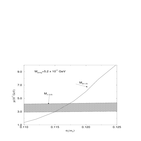
Figure 1: These are the fitted values of $M_{2}$ and $M_{3}$. The flat curve is $M_{2}$ which remains in the range $4\times 10^{13}$ GeV. Note that $M_{3}\sim M_{2}$ for the central value of $\alpha_{s}=0.118$. The shaded region gives the effect of the extra Yukawa couplings. $h_{T}(M_{X}),h_{S}(M_{X}),h_{\lambda}(M_{X})$ takes all values between 0 and 3.54

To first approximation, we let $T^{0}$ couple to $(\nu_{\mu}+\nu_{\tau})/\sqrt{2}$ and set $m_{\nu}=0.05$ eV in Eq. (1) to account for the atmospheric neutrino data. For $M_{2}\simeq 3.7\times 10^{13}$ GeV, this implies that $h_{T}\sin\beta\simeq 0.35$. To account for the solar neutrino data, we need another massive neutrino. As pointed out in Ref.[1], we have the option of choosing a heavy singlet $S\equiv(1,1,0)$ of mass $M_{1}$. This has the virtue of not affecting the existing good convergence of the gauge couplings at the string scale because it does not have any one-loop contribution. With both $T$ and $S$, we also have the bonus of CP violation in a hybrid model [9] of leptogenesis, instead of using two triplets [10].

Let $S$ couple to $s\nu_{e}+c(\nu_{\mu}-\nu_{\tau})/\sqrt{2}+\zeta(\nu_{\mu}+\nu_{\tau})/\sqrt{2}$, where $\zeta<<1$, then the neutrino mass eigenvalues are $m_{2}=h_{T}^{2}v_{2}^{2}/2M_{2}$, $m_{1}=h_{S}^{2}v_{2}^{2}/M_{1}$, and 0, with eigenstates $(\nu_{\mu}+\nu_{\tau})/\sqrt{2}$, $s\nu_{e}+c(\nu_{\mu}-\nu_{\tau})/\sqrt{2}$, and $c\nu_{e}-s(\nu_{\mu}-\nu_{\tau})/\sqrt{2}$ respectively. We can write down the neutrino mass matrix as

$$m_{\nu}=\pmatrix{s^{2}~{}m_{1}&{(c+\zeta)~{}s~{}m_{1}/\sqrt{2}}&{(-c+\zeta)~{}s~{}m_{1}/\sqrt{2}}\cr{(c+\zeta)~{}s~{}m_{1}/\sqrt{2}}&[m_{2}+(c+\zeta)^{2}m_{1}]/2&[m_{2}+(-c^{2}+\zeta^{2})m_{1}]/2\cr{(-c+\zeta)~{}s~{}m_{1}/\sqrt{2}}&[m_{2}+(-c^{2}+\zeta^{2})m_{1}]/2&[m_{2}+(-c+\zeta)^{2}m_{1}]/2}.$$ (15)

Using the sample values $m_{1}=7\times 10^{-3}$ eV, $m_{2}=5\times 10^{-2}$ eV, and $s=0.6(c=0.8)$, this implies that $(\Delta m^{2})_{atm}=2.5\times 10^{-3}$ eV², $\sin^{2}2\theta_{atm}=1$, and $(\Delta m^{2})_{sol}=4.9\times 10^{-5}$ eV², $\sin^{2}2\theta_{sol}=4s^{2}c^{2}=0.92$, in good agreement with data[11].

The couplings which are relevant for generating a lepton asymmetry of the Universe[12, 15] in this scenario are contained in

$${\cal L}=h_{T}^{i}~{}[L_{i}~{}H_{2}~{}T]+{1\over 2}M_{2}~{}[T~{}T]+h_{S}^{i}~{}[L_{i}~{}H_{2}~{}S]+{1\over 2}M_{1}~{}[S~{}S]+h_{\lambda}~{}[T~{}T~{}S],$$ (16)

where we have considered one triplet $T$ and one singlet $S$. Note that with only one triplet or only one singlet, there cannot be any CP violation. The Majorana mass terms $M_{2}$ and $M_{1}$ for the triplet and singlet superfields violate lepton number and set the scale of lepton-number violation in this model. This scale has been determined by the evolution equations for the gauge couplings to be of the order $10^{13}$ GeV. Note that all 3 new superfields $(S,T,O)$ are contained in the 24 representation of SU(5), so it is not unreasonable for them to be at the same mass scale.

Their Yukawa couplings allow the triplet and singlet superfields to decay into final states of opposite lepton number.

$$T,~{}S \to L+H_{2}~{}~{}{\rm and}~{}~{}\bar{L}+\bar{H}_{2}.$$ (17)

There are one-loop vertex diagrams interfering with the tree-level decay diagrams of $T$ and $S$, which will give rise to CP violation in these decays (see Fig. 2). This CP asymmetry will then generate a lepton asymmetry of the Universe. Unlike other models of leptogenesis where two or more heavy particles of the same type are used, there are no self-energy diagrams contributing to the CP asymmetry in this model.

Figure 2: Tree-level and one-loop vertex diagrams for the decay of the triplet $T$ resulting in a lepton asymmetry.

Assuming $M_{1}>>M_{2}$, the lepton asymmetry is generated by the decay of the triplet superfield $T$. The singlet $S$ enters in the loop diagram to give CP violation. The amount of asymmetry thus generated is given by

$$\epsilon_{L}={1\over 8\pi}\left({M_{2}\over M_{1}}\right)\zeta^{2}{{\rm Im}[(h_{S})^{2}(h_{T}^{*})^{2}]\over|h_{T}|^{2}},$$ (18)

where the factor $\zeta$ comes from the overlap between the neutrino states which couple to $T$ and $S$. In this scenario, the triplet superfield $T$ has gauge interactions, which will bring its number density to equilibrium through the interaction $T+T\to W\to L+\bar{L}$. However, the decay and the inverse decay of $T$ will be faster if we take $h^{2}_{T}(M_{2})/4\pi>>\alpha_{2}(M_{2})$. From our RGE analysis we get $\alpha_{2}(M_{2})\sim 1/25$. Since an asymmetry is only generated by a departure from equilibrium, interactions faster than expantion rate of the universe will bear an additional suppression factor in the asymmetry they generate. This factor can be estimated by numerically solving the full set of Boltzmann equations. We borrow the result from Ref.[13] that when $\Gamma/H$ is 5, the supression factor is 0.02 when it is 1000 the supression factor can be as large as $8\times 10^{-6}$. Here we make a rough estimate for our case by taking the Yukawa interaction and neglecting the gauge interaction and use an approximate supression factor,

$${\cal K}=\left({H\over\Gamma}\right)_{T=M_{2}},$$ (19)

where $H=1.7\sqrt{g_{*}}~{}T^{2}/M_{Pl}$ (with $g_{*}$ the number of relativistic degrees of freedom) is the Hubble expansion parameter and $\Gamma=h_{T}^{2}M_{2}/8\pi$ is the decay width of $T$. From our choice of numerical values for the neutrino mass matrix, we get an asymmetry

$$\epsilon_{L}=3.4\times 10^{-4}~{}\zeta^{2}\left({\sin 2\delta\over\sin^{2}\beta}\right){\cal K},$$ (20)

where $\delta$ is the relative phase between $h_{S}$ and $h_{T}$. Using $M_{2}=3.7\times 10^{13}$ GeV, $\zeta\sim 0.05$, and $\delta\sim 0.01$, we then get a lepton asymmetry $\epsilon_{L}\sim 10^{-10}$ as required. A numerical solution of the Boltzmann equations can give errors introduced in parameters $\delta$ and $\zeta$ of this simple estimate. We plan to report this analysis in a future publication. In this case, the amount of lepton asymmetry is directly related to the neutrino masses valid for atmospheric and neutrino oscillations as well as the intermediate scale required for string-scale unification. The scale of supersymmetry breaking in the hidden sector (for a particular choice of the hidden sector fields) in this scenario may also be $10^{13}$ GeV, hence this particular intermediate mass scale allows us to have a consistent description of string-scale unification, neutrino mass, leptogenesis, as well as supersymmetry breaking.

If $M_{2}>>M_{1}$, it will be the decay of the singlet $S$ which generates the lepton asymmetry. In this case the singlet does not have any gauge interactions but its Yukawa interaction will be similar to that of the triplet in the previous case. Hence the amount of lepton asymmetry is again similar, except that the roles of $M_{1}$ and $M_{2}$ are reversed. Finally, this lepton asymmetry gets converted into the present baryon asymmetry of the Universe from the action of the $B+L$ violating electroweak sphalerons [14], in analogy with the canonical leptogensis decay of heavy right-handed neutrinos [15].

Finally we would consider restrictions imposed by inflationary scenarios as lepton asymmetry should be created after the reheating starts after the inflation. For example if lepton number violation takes place at $10^{12}$ GeV and the upper bound on reheating temperature is $10^{6}$ GeV it rules out the corresponding mechanism of leptogenesis. In our case the mass scale $m_{3/2}$ is closely related to $M_{I}$ and $m_{string}$ via $M_{I}\sim M_{string}^{2/3}m^{1/3}_{3/2}$. Furthermore the values used in the RGE analysis does not include threshold effects and “smoothed” threshold functions. The value of $M_{I}$ should be taken at best as a guiding value. Taking $m_{3/2}\geq 5(200)$ TeV we get $M_{I}\geq 1.1(3.8)\times 10^{13}$ GeV which is consistent with value of the triplet mass obtained in Fig. 1. Such a heavy gravitino should decay otherwise it will over-close the universe. Now let us say that the gravitino decays predominantly to photon and photino. Upper bound on the reheating temperature depends on the mass of gravitino. We see from Figure (17) of the reference [16] that for $m_{3/2}$ more than 5 TeV, reheating temperature upper-bound is more than $10^{13}$ GeV. Furthermore the produced photon may further produce hadrons[17]. In that case we get from Figure (14) of reference [18] that for $m_{3/2}$ more than 200 TeV, the reheating upper-bound is more than $10^{13}$ GeV. In both these cases our scenario is consistent with post inflationary reheating. Infact note that from RGE analysis we get values of $M_{I}$ which actually gives $m_{3/2}$ in the 200 TeV range in a natural way. However the dominant decay mode of the gravitino may not be photon and photino. The case where the gravitino decays to a neutrino and sneutrino, when it is kinematically allowed, has been studied in [19]. In this case neutrinos and sneutrinos produce photons in cascade those interact and change predicted abundance of the light elements which may differ from the observed values of the abundance of light elements. In this case the upper bound on the reheating temperature is tighter, which is around $10^{12}$ GeV. This intermediate scale will produce a smaller gravitino mass unless the string scale is lowered. In this case the present scenario would be in trouble. Also, one must remember that there is experimental uncertainty in the determination of the abundance of light elements themselves such as the primordial fraction of ⁴He[22]. Finally in various supersymmetric extensions of the standard model one can have light axinos in the KeV range and gravitino decays to axino. In such scenarios the upper bound on the reheating increases to $10^{15}$ GeV[20].

A valid case can be made for larger soft masses of 100 TeV range as it is good for suppressing supersymmetric flavor changing neutran current and CP violation[21] problems. In any case both supersymmetry and neutrino mass are physics beyond the standard model. In our paper we have addressed neutrino mass and a possibility of leptogenesis. In this model renormalization group analysis has resulted an intermediate scale which gives $m_{3/2}$ in the range of 100 TeV. As long as there is no fundamental reason why $m_{3/2}$ cannot be in the 100 TeV range our model stands correct.

In summary this is a scenario where the mass of the adjoint superfields $S\equiv(1,1,0),T\equiv(1,3,0)$ and $O\equiv(8,1,0)$ are all approximately degenerate at $M_{I}\sim M_{string}^{2/3}m^{1/3}_{3/2}\sim 10^{13}$ GeV. This scenario has been studied in the literature in the context of string unification where it has been shown that the unification of gauge couplings occur at $5.2\times 10^{17}$ GeV. In this paper we have shown that this scenario can lead to a neutrino mass matrix which produces $(\Delta m^{2})_{atm}=2.5\times 10^{-3}$ eV², $\sin^{2}2\theta_{atm}=1$, and $(\Delta m^{2})_{sol}=4.9\times 10^{-5}$ eV², $\sin^{2}2\theta_{sol}=0.92$. This is in good agreement with atmospheric and solar neutrino data. Furthermore, there are two ways that the triplet superfield $T$ may decay to $L$ and $H_{2}$, and in one of which the singlet $S$ resides in a loop. The interference of these decay amplitudes allows for the CP violation needed for leptogenesis. We have shown that after we take into account the suppression in the generated lepton asymmetry due an approximate equilibrium condition between the forward and inverse decays of $T$, the final lepton asymmetry emerges in the range $\epsilon_{L}\sim 10^{-10}$ as required.

This work was supported in part by the U. S. Department of Energy under Grant No. DE-FG03-94ER40837. BB thanks Probir Roy for communications on gravitino decay modes.

References

- [1] E. Ma, Phys. Rev. Lett 81, 1171 (1998).
- [2] M. Gell-Mann, P. Rammond and R. Slansky, in Supergravity, edited by P. Van Nieuwenhuizen and D. Z. Freedman, (North-Holland, Amsterdam, 1979), p. 315; T. Yanagida, in Proceedings of the Workshop on the UNified Theory and the Baryon Number in the Universe, edited by O. Sawada and A. Sugamoto (KEK, Tsukuba, Japan, 1979), p. 95; R. N. Mohapatra and G. Senjanović. Phys. Rev. Lett 44, 912 (1980).
- [3] C. Bachas, C. Fabre, and T. Yanagida, Phys. Lett. B370, 49 (1996); M. Bastero-Gil and B. Brahmachari, Phys. Lett. B403, 51 (1997); T. Han, T. Yanagida, and R. J. Zhang, Phys. Rev. D58 095011 (1998); J.L. Chkareuli, C.D. Froggatt, I.G. Gogoladze, A.B. Kobakhidze, Nucl. Phys. B594 23 (2001).
- [4] S. Fukuda et al., Super-Kamiokande Collaboration, Phys. Rev. Lett. 85, 3999 (2000) and references therein.
- [5] Y. Fukuda et al., Super-Kamiokande Collaboration, Phys. Rev. Lett. 81, 1158 (1998); 82, 1810, 2430 (1999).
- [6] P. Ginsparg, Phys. Lett. B197, 139 (1987); V. Kaplunovsky, Nucl. Phys. B307, 145 (1988); ibid. B382, 436 (1992).
- [7] K. Inoue et al., Prog. Theor. Phys. 68, 927, (1982); ibid. 67, 1889 (1982). J. E. Bjorkman and D. R. T. Jones, Nucl. Phys. B259, 533 (1985); A. E. Faraggi, B. Grinstein, S. Meshkov, Phys. Rev. D47,5018 (1993).
- [8] K. S. Babu and E. Ma, Phys. Lett. B144, 381 (1984).
- [9] P. J. O’Donnell and U. Sarkar, Phys. Rev. D49, 2118 (1994); E. J. Chun and S. K. Kang, Phys. Rev. D63, 097902 (2001); A. de Gouvea and J. W. F. Valle, Phys. Lett. B501, 115 (2001).
- [10] E. Ma and U. Sarkar, Phys. Rev. Lett 80, 5716 (1998); T. Hambye, E. Ma, and U. Sarkar, Nucl. Phys. B602, 23 (2001).
- [11] Super-Kamiokande Collaboration (S. Fukuda et al.); e-Print Archive: hep-ex/0103033; J. N. Bahcall, P. I. Krastev, A. Yu. Smirnov, JHEP 0105:015,2001; S. Choubey, S. Goswami, N. Gupta, D.P. Roy, e-Print Archive: hep-ph/0103318; G.L. Fogli, E. Lisi, A. Marrone, e-Print Archive: hep-ph/0105139; Super-Kamiokande Collaboration (Toshiyuki Toshito for the collaboration), e-Print Archive: hep-ex/0105023; S. Choubey, S. Goswami, K. Kar, e-Print Archive: hep-ph/0004100.
- [12] M.A. Luty, Phys. Rev. D45 455 (1992). W. Buchmuller and M. Plumacher, Int. J. Mod. Phys. A15, 5047 (2000).
- [13] J. Faridani, S. Lola, P. J. O’Donnell, U. Sarkar Eur. Phys. J. C7 543 (1999).
- [14] V. A. Kuzmin, V. A. Rubakov, and M. E. Shaposhnikov, Phys. Lett. 155B, 36 (1985).
- [15] M. Fukugita and T. Yanagida, Phys. Lett. 174B, 45 (1986).
- [16] E. Holtmann, M. Kawasaki, K. Kohri, T. Moroi, Phys. Rev. D60, 023506,1999
- [17] M. H. Reno and D. Seckel, Phys. Rev. D 37 3441 (1998); J. R. Ellis, G. B. Gelmini, J. L. Lopez, D. V. Nanopoulos and S. Sarkar, Nucl. Phys. B 373 399 (1992)
- [18] K. Kohri, Phys. Rev. D64, 043515 (2001).
- [19] M. Kawasaki, T. Moroi, Phys. Lett. B346 27, (1995)
- [20] T. Asaka, T. Yanagida, Phys. Lett. B494, 297 (2000)
- [21] See for example, M. Misiak, S. Pokorski, J. Rosiek ,In the Review Volume ’Heavy Flavors II’, eds. A.J. Buras and M. Lindner, Advanced Series on Directions in High-Energy Physics, World Scientific Publishing Co., Singapore. e-Print Archive: hep-ph/9703442 and references therein.
- [22] Y. I. Izotov, T. X. Thuan and V. A. Lipovetsky, Astrophys. J. 435, 467 (1994).