How Protons Shatter Colored Glass

Abstract

We consider the implications of the Color Glass Condensate for the central region of $p+A$ collisions. We compute the $k_{\perp}$ distribution of radiated gluons and their rapidity distribution ${\rm d}N/{\rm d}y$ analytically, both in the perturbative regime and in the region between the two saturation momenta. We find an analytic expression for the number of produced gluons which is valid when the saturation momentum of the proton is much less than that of the nucleus. We discuss the scaling of the produced multiplicity with $A$. We show that the slope of the rapidity density ${\rm d}N/{\rm d}y$ provides an experimental measure for the renormalization-group evolution of the color charge density of the Color Glass Condensate (CGC). We also argue that these results are easily generalized to collisions of nuclei of different $A$ at central rapidity, or with the same $A$ but at a rapidity far from the central region.

I Introduction

The color field of a strongly Lorentz boosted hadron can be described as a classical color field [1], so long as one has a high enough density of gluons such that the field modes have very large occupation numbers. The typical transverse momentum scale for which the field modes have large occupation number will be called $Q_{s}$, the saturation momentum. Seen with a resolution scale of $Q_{s}$, the collision of two hadrons (say pions, protons, or nuclei) at very high energy can be viewed as two (highly Lorentz contracted) sources of color charge propagating along the light-cone. Renormalization group evolution in rapidity leads to a longitudinal extension of the source. That is, the charge distribution is spread out on a scale given by the characteristic longitudinal momentum of the “hard” particles which generate the source of color charge entering the Yang-Mills equation for the “soft” modes.

The field in front of and behind each “sheet” of charge is a pure gauge [1]. The color electric and magnetic fields associated with these pure gauge vector potentials vanish, except in the sheet where the vector potential is discontinuous (on a scale larger than the longitudinal spread of the color charge source). When the two sheets collide, corresponding to the tip of the light-cone, the two charge sheets interact. This produces radiation in the forward light cone.

The point of our paper is to compute this radiation for collisions of particles with different saturation momentum scales. This problem turns out to be more tractable than that of collisions of two particles with equal saturation scales. For example, to compute the production of particles in the central region of equal $A$ nuclear collisions, one must perform intensive numerical computations [2]. If one collides protons with nuclei at very high energies and studies the central region of particle production, there are two scales, the saturation momentum of the proton and that of the nucleus. In the limit where $\Lambda_{QCD}\ll Q_{s}^{\rm proton}\ll Q_{s}^{A}$, we shall see that the problem simplifies, and one can obtain analytic results for quantities such as the total multiplicity density of gluons at zero rapidity.

The saturation momentum squared is proportional to the total number of gluons in the hadron wavefunction at rapidities larger than that at which we compute the production of particles. One could introduce an asymmetry in the saturation scales by considering equal $A$ nuclear collisions far from the central rapidity region. Alternatively, one could consider collisions of different nuclei, or various combinations of the above. In this sense, the proton in the $p+A$ scattering case which we consider should be thought of as a generic acronym for asymmetric nuclear collisions in either baryon number or rapidity.

We shall specifically consider the situation where the source propagating along the $x^{+}=(t+z)/\sqrt{2}$ axis is much weaker than that propagating along the $x^{-}=(t-z)/\sqrt{2}$ axis. In such a case, the saturation momentum scale $Q_{s}^{(1)}$ on which source one can be viewed as a classical field is smaller than the corresponding scale for source two, $Q_{s}^{(2)}$. This fact has a very interesting consequence. Namely, we expect three distinct regions in transverse momentum. At large transverse momentum, $k_{\perp}>Q_{s}^{(2)}$, both fields are weak. Thus, perturbation theory should be a valid approximation in this regime [3, 4, 5]. On the other hand, for $Q_{s}^{(2)}>k_{\perp}>Q_{s}^{(1)}$, the field one is weak, and can be treated perturbatively; but field two is “saturated”, that is, the field strength $F^{\mu\nu}={\cal O}(1/g)$ has attained maximum strength [1, 6], and is in the non-linear regime. In that regime of transverse momentum, field two can not be treated as a small perturbation, even if $Q_{s}^{(2)}\gg\Lambda_{\rm QCD}$ and the coupling $\alpha_{s}(Q_{s}^{(2)})\ll 1$ is weak. Those non-linearities modify the transverse momentum distribution of radiation produced due to the interaction. Our goal here is to compute the distribution in the intermediate regime $Q_{s}^{(2)}>k_{\perp}>Q_{s}^{(1)}$. Finally, at an even smaller transverse momentum $<Q_{s}^{(1)}$, both fields are strong. In this region we expect a flat $k_{\perp}$ distribution, up to logarithms of $k_{\perp}^{2}$. However, we can presently not compute the distribution in that region analytically, but it has been obtained numerically [2].

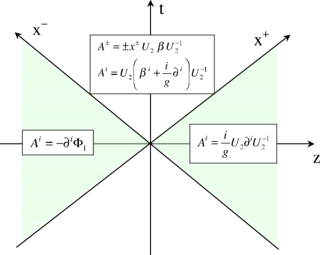
FIG. 1.: The solutions of the Yang-Mills equations in the various parts of the light-cone. The charge distributions propagate along the $x^{-}$, $x^{+}$ axes. In the space-like regions behind the charge distributions the fields are just gauge transformations of vacuum fields, rotated by the respective charge densities of the sources. In the forward light-cone, the field at time $\rightarrow\infty$ is given by gauge rotated plane wave solutions $\beta$ and $\beta^{i}$.

The solution of the nonabelian Yang-Mills equations is illustrated in Fig. 1. The two color-charge distributions propagate along the $x^{-}$, $x^{+}$ axes. The fields $A^{i}$ in the space-like regions behind them are just gauge rotated vacuum fields, and $A^{\pm}=0$ there.

For an abelian gauge group (electrodynamics) the field in the forward light-cone is just the sum of the two pure-gauge fields behind the propagating charge distributions. It is also just a gauge rotated vacuum field, and so no radiation occurs (if recoil is neglected). For a non-abelian gauge group (chromodynamics) the sum of two pure gauges is not a pure gauge, and radiation occurs at the classical level, even when recoil is neglected. At asymptotic times, the field in the forward light-cone must be given by gauge rotated plane waves. In a leading order perturbative computation [3, 4, 5] those gauge rotations can be expanded to first order in the gauge potentials. However, in order to reach into the non-linear “saturation regime” we must account for the interaction of the radiation field with the fields of the color-charge distributions on the light-cone to all orders. A numerical approach to this problem has been used in ref. [2] for collisions of equal-size nuclei, and at midrapidity. For current-nucleus interactions (Deep Inelastic Scattering off large nuclei) the distribution function of produced gluons in the fragmentation region has been obtained analytically (via a diagrammatic approach) in [7], where the authors also discuss the generalization of their result to $p+A$ collisions. In the central rapidity region (the region $z\ll t$ in Fig. 1) one should also account for the renormalization group (RG) evolution of the CGC color charge density per unit transverse area [8, 9]. The purpose of this paper is to derive analytically an explicit expression for the transverse momentum and rapidity distribution of produced gluons in $A_{1}+A_{2}$ collisions at high energy, valid at all rapidities where the CGC color charge density including RG evolution is much larger for the source $A_{2}$ than for $A_{1}$. Our explicit result for ${\rm d}N/{\rm d}k_{\perp}^{2}{\rm d}y$ shows that the transverse momentum distribution is modified from a $\sim 1/k_{\perp}^{4}$ behavior in the perturbative regime (high $k_{\perp}$) to $\sim 1/k_{\perp}^{2}$ in the region where $k_{\perp}$ is between the saturation scales for the two sources. Furthermore, we show that the slope of the multiplicity per unit of rapidity, ${\rm d}N/{\rm d}y$, provides an experimental measure for the RG evolution of the CGC color charge density.

This article is organized as follows. In section II we derive the transverse momentum and rapidity distribution of the radiated gluons to all orders in the field of the large nucleus. We do this by solving the Yang-Mills equations with the appropriate boundary conditions. This section is somewhat technical and can be skipped by readers interested only in the results relevant for phenomenology. In section III we discuss the most important features of the radiation spectrum in the perturbative regime (high transverse momentum) and in the “saturation regime”, including the $A$-scaling and the evolution in rapidity. We outline possible ways of measuring experimentally the RG evolution of the color charge density of the CGC. We summarize in section IV.

II The Distribution of Produced Gluons

In this section, we shall first solve the Yang-Mills equations in coordinate space. We assume that in the forward light-cone the vector potential depends only on the transverse coordinate $x_{\perp}$ and on proper time, $\tau=\sqrt{t^{2}-z^{2}}\equiv\sqrt{2x^{+}x^{-}}$ (which is invariant under longitudinal Lorentz boosts), but not on rapidity $y=\log(x^{+}/x^{-})/2$. When performing the path integral over the “hard” source for the classical color field in eq. (53) we shall explicitly consider the dependence on rapidity.

In the space-like regions the transverse fields are pure gauges [1],

$$\alpha_{m}^{i} = -\frac{1}{ig}U_{m}(x_{\perp})\partial^{i}U^{\dagger}_{m}(x_{\perp})$$ (1)

$$= -\frac{1}{ig}e^{-ig\Phi_{m}(x_{\perp})}\partial^{i}e^{ig\Phi_{m}(x_{\perp})}\quad(m=1,2)~{}.$$ (2)

The fields $\Phi_{m}$ satisfy

$$-\nabla^{2}_{\perp}\Phi_{m}=g\rho_{m}(x_{\perp})~{}.$$ (3)

We take the distribution of the sources of the gluon color field for each nucleus as a Gaussian according to the McLerran-Venugopalan model,

$$\int{\cal D}\rho_{1}\,{\cal D}\rho_{2}\;\exp\left(-F_{1}[\rho_{1}]-F_{2}[\rho_{2}]\right)~{},$$ (4)

where

$$F_{i}[\rho_{i}]=\int{\rm d}y\,{\rm d}^{2}x_{\perp}\;{\rm tr}\,\rho_{i}^{2}(x_{\perp},y)/\mu^{2}_{i}(y)~{}.$$ (5)

The quantity $\mu^{2}(y)$ is the color charge squared per unit rapidity and per unit transverse area scaled by $N_{c}^{2}-1$. It can be related to the gluon distribution function with known coefficients, as shown in Ref. [4]. It will turn out that the radiation distribution depends only on integrals over $\mu^{2}(y)$, i.e. the total color charge squared from rapidities greater than that at which we are interested in computation.

The field $\Phi_{1}$ will be assumed to be weak such that the exponentials in eq. (2) can be expanded to leading order,

$$\alpha_{1}^{i}=-\partial^{i}\Phi_{1}+{\cal O}(\Phi_{1}^{2})~{}.$$ (6)

In the forward light-cone we write the transverse and $\pm$ components of the gauge field as

$$A^{i}(\tau,x_{\perp}) = \alpha_{3}^{i}(\tau,x_{\perp})~{},$$ (7)

$$A^{\pm}(\tau,x_{\perp}) = \pm x^{\pm}\alpha(\tau,x_{\perp})~{},$$ (8)

corresponding to the gauge condition

$$x^{+}A^{-}+x^{-}A^{+}=0~{}.$$ (9)

Thus, our ansatz for the gauge fields is

$$A^{i}(\tau,x_{\perp}) = \alpha_{3}^{i}(\tau,x_{\perp})\Theta(x^{-})\Theta(x^{+})$$ (10)

$$+ \alpha_{1}^{i}(x_{\perp})\Theta(x^{-})\Theta(-x^{+})$$ (11)

$$+ \alpha_{2}^{i}(x_{\perp})\Theta(-x^{-})\Theta(x^{+})~{},$$ (12)

$$A^{\pm}(\tau,x_{\perp}) = \pm x^{\pm}\alpha(\tau,x_{\perp})\Theta(x^{-})\Theta(x^{+})~{}.$$ (13)

Next, we determine the boundary conditions for $x^{-},x^{+}\rightarrow 0$. In that limit,

$$\left[D_{+},F^{+i}\right]+\left[D_{-},F^{-i}\right]=2\delta(x^{-})\delta(x^{+})\left(\alpha_{3}^{i}-\alpha_{1}^{i}-\alpha_{2}^{i}\right)~{}.$$ (14)

(The contribution from $[D_{j},F^{ji}]$ is not singular at $x^{+}=x^{-}=0$.) For this term to vanish identically we must satisfy the boundary condition

$$\alpha_{3}^{i}(\tau=0,x_{\perp})=\alpha_{1}^{i}(x_{\perp})+\alpha_{2}^{i}(x_{\perp})~{},$$ (15)

as found before in [3, 4].

Using (15), the equation

$$\left[D_{\mu},F^{\mu+}\right]=J^{+}\equiv\delta(x^{-})\,g\rho_{1}(x_{\perp})~{},$$ (16)

where $\rho_{1}$ is the charge density per transverse area in nucleus 1, gives for $x^{+},x^{-}\rightarrow 0$

$$\delta(x^{-})\left\{2\alpha\Theta(x^{+})+\partial_{i}\alpha_{1}^{i}-\Theta(x^{+})\,ig\left[\alpha_{1}^{i},\alpha_{2}^{i}\right]\right\}$$ (17)

$$= \delta(x^{-})\,\partial_{i}\alpha_{1}^{i}~{}.$$ (18)

That requires the matching condition [3, 4]

$$\alpha(\tau=0,x_{\perp})=\frac{ig}{2}\left[\alpha_{1}^{i}(x_{\perp}),\alpha_{2}^{i}(x_{\perp})\right]~{}.$$ (19)

We now determine the solution in the forward light-cone, $x^{+},x^{-}>0$. $[D_{\mu},F^{\mu\nu}]=0$ becomes [3]

$$\frac{1}{\tau^{3}}\partial_{\tau}\tau^{3}\partial_{\tau}\alpha-\left[D^{i},\left[D_{i},\alpha\right]\right] = 0~{},$$ (20)

$$\frac{1}{\tau}\left[D_{i},\partial_{\tau}\alpha_{3}^{i}\right]+ig\tau\left[\alpha,\partial_{\tau}\alpha\right] = 0~{},$$ (21)

$$\frac{1}{\tau}\partial_{\tau}\tau\partial_{\tau}\alpha_{3}^{i}-ig\tau^{2}\left[\alpha,\left[D^{i},\alpha\right]\right]-\left[D^{j},F^{ji}\right] = 0~{}.$$ (22)

We assume that the field of the second nucleus is much stronger than the radiation field, and so linearize the equations of motion in $\alpha$. (Note that $\alpha\rightarrow 0$ if source one becomes arbitrarily weak, as no radiation occurs in the single nucleus case.) That amounts to dropping the second terms in eqs. (21,22). We perform a gauge rotation

$$\alpha(\tau,x_{\perp}) = U_{2}(x_{\perp})\beta(\tau,x_{\perp})U_{2}^{\dagger}(x_{\perp})~{},$$ (23)

$$\alpha_{3}^{i}(\tau,x_{\perp}) = U_{2}(x_{\perp})\left(\beta^{i}(\tau,x_{\perp})-\frac{1}{ig}\partial^{i}\right)U_{2}^{\dagger}(x_{\perp})~{},$$ (24)

with $U_{2}=\exp(-ig\Phi_{2})$ as defined in (2). Then $[D^{i},\cdot]$ becomes the ordinary derivative $\partial^{i}$ up to corrections of order ${\cal O}(\beta^{i})$ which do not show up in the linearized equations of motion,

$$\frac{1}{\tau^{3}}\partial_{\tau}\tau^{3}\partial_{\tau}\beta-\partial^{i}\partial_{i}\beta = 0~{},$$ (25)

$$\partial_{\tau}\partial_{i}\beta^{i} = 0~{},$$ (26)

$$\frac{1}{\tau}\partial_{\tau}\tau\partial_{\tau}\beta^{i}-\left(\partial^{k}\partial_{k}\delta^{ij}-\partial^{i}\partial^{j}\right)\beta^{j} = 0~{}.$$ (27)

Gauge rotating the boundary conditions (15,19) gives

$$\beta^{i}(\tau=0,x_{\perp}) = U_{2}^{\dagger}(x_{\perp})\alpha_{1}^{i}(x_{\perp})U_{2}(x_{\perp})~{},$$ (28)

$$\beta(\tau=0,x_{\perp}) =$$ (30)

$$\frac{ig}{2}U_{2}^{\dagger}(x_{\perp})\left[\alpha_{1}^{i}(x_{\perp}),\alpha_{2}^{i}(x_{\perp})\right]U_{2}(x_{\perp})~{}.$$

From (26), $\partial_{i}\beta^{i}(\tau,x_{\perp})$ is time independent. We can thus write

$$\beta^{i}(\tau,x_{\perp})=\epsilon^{il}\partial^{l}\chi(\tau,x_{\perp})+\partial^{i}\Lambda(x_{\perp})~{},$$ (31)

where $\epsilon^{il}$ is the Levi-Civita tensor in two dimensions. The first term contributes to the curl while the second contributes to the divergence of $\beta^{i}$. This ansatz for $\beta^{i}$ makes (26) an identity. The equations of motion (25-27) now read

$$\frac{1}{\tau^{3}}\partial_{\tau}\tau^{3}\partial_{\tau}\beta-\partial^{i}\partial_{i}\beta = 0~{},$$ (32)

$$\frac{1}{\tau}\partial_{\tau}\tau\partial_{\tau}\tilde{\chi}-\partial^{i}\partial_{i}\tilde{\chi} = 0~{},$$ (33)

where $\tilde{\chi}=-\partial^{j}\partial_{j}\chi$. The boundary condition for $\tilde{\chi}$ can be obtained by noting that $\tilde{\chi}=\epsilon^{ij}\partial^{j}\beta^{i}$,

$$\tilde{\chi}(\tau=0,x_{\perp})=\epsilon^{ij}\partial^{j}U_{2}^{\dagger}(x_{\perp})\alpha_{1}^{i}(x_{\perp})U_{2}(x_{\perp})~{}.$$ (34)

The equations of motion (32,33) are solved by a superposition of Bessel functions,

$$\beta(\tau,x_{\perp}) = \int\frac{{\rm d}^{2}k_{\perp}}{(2\pi)^{2}}e^{ik_{\perp}\cdot x_{\perp}}b_{1}(k_{\perp})\frac{1}{\omega\tau}J_{1}(\omega\tau)~{},$$ (35)

$$\tilde{\chi}(\tau,x_{\perp}) = \int\frac{{\rm d}^{2}k_{\perp}}{(2\pi)^{2}}e^{ik_{\perp}\cdot x_{\perp}}b_{2}(k_{\perp})J_{0}(\omega\tau)~{}.$$ (36)

The functions $b_{1}(k_{\perp})$, $b_{2}(k_{\perp})$ are determined in coordinate space by the boundary conditions for the fields at $\tau=0$:

$$b_{2}(x_{\perp}) = \int\frac{{\rm d}^{2}k_{\perp}}{(2\pi)^{2}}e^{ik_{\perp}\cdot x_{\perp}}b_{2}(k_{\perp})=\tilde{\chi}(\tau=0,x_{\perp})~{},$$ (37)

$$b_{1}(x_{\perp}) = \int\frac{{\rm d}^{2}k_{\perp}}{(2\pi)^{2}}e^{ik_{\perp}\cdot x_{\perp}}b_{1}(k_{\perp})=2\beta(\tau=0,x_{\perp})~{}.$$ (38)

This follows from the expansion of $J_{\nu}(x)$ for small $x$: $J_{\nu}(x)\simeq(x/2)^{\nu}/\nu!$. Asymptotically, for $x\rightarrow\infty$, the Bessel functions are $J_{\nu}(x)\simeq\sqrt{2/\pi x}\cos(x-\nu\pi/2-\pi/4)$. Also, for time $\tau\rightarrow\infty$ we assume free fields, $\omega=|\vec{k}_{\perp}|$. Then, comparing the solutions (35,36) for $\tau\rightarrow\infty$ to plane waves [3],

$$\beta(\tau\rightarrow\infty,x_{\perp}) = \int\frac{{\rm d}^{2}k_{\perp}}{(2\pi)^{2}}\frac{1}{\sqrt{2\omega\tau^{3}}}$$ (40)

$$\times\left\{a_{1}(k_{\perp})e^{ik_{\perp}\cdot x_{\perp}-i\omega\tau}+c.c.\right\}~{},$$

$$\beta^{i}(\tau\rightarrow\infty,x_{\perp}) = \int\frac{{\rm d}^{2}k_{\perp}}{(2\pi)^{2}}\frac{1}{\sqrt{2\omega\tau}}\frac{\epsilon^{il}k_{\perp}^{l}}{\omega}$$ (42)

$$\times\left\{a_{2}e^{ik_{\perp}\cdot x_{\perp}-i\omega\tau}+c.c.\right\}~{},$$

yields for purely imaginary $b_{2}(k_{\perp})$ and real $b_{1}(k_{\perp})$:

$$a_{1}(k_{\perp}) = \frac{1}{\sqrt{\pi}k_{\perp}}b_{1}(k_{\perp})e^{3\pi i/4}$$ (43)

$$= \frac{ig}{\sqrt{\pi}k_{\perp}}e^{3\pi i/4}\int{\rm d}^{2}x_{\perp}e^{-ik_{\perp}\cdot x_{\perp}}$$ (45)

$$\times U_{2}^{\dagger}(x_{\perp})\left[\alpha_{1}^{i}(x_{\perp}),\alpha_{2}^{i}(x_{\perp})\right]U_{2}(x_{\perp})~{},$$

$$a_{2}(k_{\perp}) = \frac{1}{\sqrt{\pi}k_{\perp}}b_{2}(k_{\perp})e^{i\pi/4}$$ (46)

$$= \frac{i}{\sqrt{\pi}k_{\perp}}e^{i\pi/4}\int{\rm d}^{2}x_{\perp}e^{-ik_{\perp}\cdot x_{\perp}}$$ (48)

$$\times\epsilon^{ij}\partial^{j}U_{2}^{\dagger}(x_{\perp})\alpha_{1}^{i}(x_{\perp})U_{2}(x_{\perp})~{}.$$

To simplify $a_{1}$, recall from (2) that $\alpha_{2}^{i}=U_{2}(-1/ig)\partial^{i}U_{2}^{\dagger}$. Therefore,

$$igU_{2}^{\dagger}\left[\alpha_{1}^{i},\alpha_{2}^{i}\right]U_{2} = \partial^{i}U_{2}^{\dagger}\alpha_{1}^{i}U_{2}-U_{2}^{\dagger}\left(\partial^{i}\alpha_{1}^{i}\right)U_{2}$$ (49)

$$= \alpha_{1}^{a,i}\partial^{i}U_{2}^{\dagger}t^{a}U_{2}~{}.$$ (50)

Let us evaluate ${\rm tr}|a_{2}|^{2}$ first. Squaring the amplitude and taking the trace yields

$${\rm tr}|a_{2}|^{2} = \frac{1}{{\pi}k_{\perp}^{2}}\int{\rm d}^{2}x_{\perp}{\rm d}^{2}z_{\perp}e^{-ik_{\perp}\cdot(x_{\perp}-z_{\perp})}$$ (52)

$$\times\epsilon^{ij}\epsilon^{kl}\partial_{x}^{j}\partial_{z}^{l}\,{\rm tr}\langle A^{i}(x_{\perp},y)A^{k}(z_{\perp},y)\rangle_{\Phi_{1},\Phi_{2}}~{}.$$

Here, $y$ denotes the rapidity. The averaging is with respect to the gauge potentials $\Phi_{1}$ and $\Phi_{2}$, assuming a Gaussian weight [1, 9]:

$$\langle O\rangle_{\Phi} = \int\!\!{\cal D}\Phi\,O(\Phi)$$ (53)

$$\times \exp\left[-\int{\rm d}y^{\prime}\int{\rm d}^{2}x_{\perp}\frac{{\rm tr}\left(\nabla^{2}_{\perp}\Phi(x_{\perp},y^{\prime})\right)^{2}}{g^{2}\mu^{2}(x_{\perp},y^{\prime})}\right]~{}.$$ (54)

When averaging over $\Phi_{2}$, the $y^{\prime}$-integral extends from $-\infty$ (or some large negative rapidity beyond which the source vanishes) to the rapidity of the produced gluons, $y$. Vice versa, when averaging over $\Phi_{1}$ it goes from $y$ to $+\infty$.

We now have to compute the correlation function

$${\rm tr}\langle A^{i}(x_{\perp},y)A^{k}(z_{\perp},y)\rangle_{\Phi_{1},\Phi_{2}}$$ (55)

with

$$A^{i}(x_{\perp},y)=U_{2}^{\dagger}(x_{\perp},y)\left(\partial^{i}\Phi_{1}(x_{\perp},y)\right)U_{2}(x_{\perp},y)~{}.$$ (56)

The average over $\Phi_{1}$ in eqs. (52,55) can be performed right away. From (53) we have [9]

$$\partial_{x}^{i}\partial_{z}^{k}\langle\Phi_{1}^{a}(x_{\perp},y)\Phi_{1}^{b}(z_{\perp},y)\rangle_{\Phi_{1}}$$ (57)

$$= g^{2}\delta^{ab}\int^{\infty}_{y}\!\!{\rm d}y^{\prime}\,\mu_{1}^{2}(y^{\prime})\,\partial_{x}^{i}\partial_{z}^{k}\gamma(u_{\perp})$$ (58)

$$= g^{2}\delta^{ab}\chi_{1}(y)\,\partial_{x}^{i}\partial_{z}^{k}\gamma(u_{\perp})~{},$$ (59)

with $u_{\perp}\equiv x_{\perp}-z_{\perp}$. Also, we defined the total charge squared at rapidity $y$ induced by the source from rapidities $[y,\infty]$ (not to be confused with the auxilliary fields $\chi$, $\tilde{\chi}$ used above in intermediate steps of the calculation),

$$\chi_{1}(y)=\int^{\infty}_{y}{\rm d}y^{\prime}\,\mu_{1}^{2}(y^{\prime})~{}.$$ (60)

The tadpole-subtracted propagator is [9]

$$\gamma(x_{\perp})=\frac{1}{8\pi}x_{\perp}^{2}\log x_{\perp}^{2}\Lambda_{\rm QCD}^{2}~{}.$$ (61)

Also, in (59) we assumed slow variation of $\mu_{1}$ over the relevant transverse scales, and so neglect derivatives of it.

We are left with

$${\rm tr}\langle U^{\dagger}_{2}(x_{\perp},y)t^{a}U_{2}(x_{\perp},y)U^{\dagger}_{2}(z_{\perp},y)t^{a}U_{2}(z_{\perp},y)\rangle_{\Phi_{2}}~{}.$$ (62)

The most efficient way to evaluate this expression is to note that

$$\left(U^{\dagger}_{2}(x_{\perp},y)t^{a}U_{2}(x_{\perp},y)\right)_{\alpha\beta}=\left(t^{a^{\prime}}\right)_{\alpha\beta}U_{\rm adj}^{a^{\prime}a}(x_{\perp})=$$ (63)

$$\left(t^{a^{\prime}}\right)_{\alpha\beta}\left({\cal P}\exp\left(ig\int^{y}_{-\infty}\!\!{\rm d}y^{\prime}\,T^{b}\Phi_{2}^{b}(x_{\perp},y^{\prime})\right)\right)^{a^{\prime}a}~{}.$$ (64)

The path ordered exponential can be expanded as

$$1 + ig\int^{y}_{-\infty}{\rm d}y^{\prime}T^{b}_{a^{\prime}a}\Phi_{2}^{b}(x_{\perp},y^{\prime})$$ (65)

$$+ (ig)^{2}\int^{y}_{-\infty}\!\!\!\!{\rm d}y^{\prime}\int^{y^{\prime}}_{-\infty}\!\!\!\!{\rm d}y^{\prime\prime}T^{b}_{a^{\prime}d}T^{c}_{da}\Phi_{2}^{b}(x_{\perp},y^{\prime})\Phi_{2}^{c}(x_{\perp},y^{\prime\prime})$$ (66)

$$+ \cdots$$ (67)

According to (62) we have to multiply two such expressions, one at $x_{\perp}$ and the other at $z_{\perp}$. The zeroth order is of course trivial. The contribution to ${\cal O}(g^{2})$ arises from the product of the two ${\cal O}(g)$ terms in (67) because tadpoles only enter via a subtraction of the propagator, $\gamma(u_{\perp})$, at $u_{\perp}=0$ [9]. We find

$$(ig)^{2}\!\!\!\int^{y}_{-\infty}\!\!\!\!{\rm d}y^{\prime}\!\!\!\int^{y}_{-\infty}\!\!\!\!{\rm d}\bar{y}^{\prime}\,T^{b}_{a^{\prime}a}T^{b^{\prime}}_{a^{\prime}a}\left\langle\Phi_{2}^{b}(x_{\perp},y^{\prime})\Phi_{2}^{b^{\prime}}(z_{\perp},\bar{y}^{\prime})\right\rangle_{\Phi_{2}}$$ (68)

$$= {g^{2}}N_{c}\,\delta^{bb^{\prime}}\!\!\!\int^{y}_{-\infty}\!\!\!\!{\rm d}y^{\prime}\!\!\!\int^{y}_{-\infty}\!\!\!\!{\rm d}\bar{y}^{\prime}\left\langle\Phi_{2}^{b}(x_{\perp},y^{\prime})\Phi_{2}^{b}(z_{\perp},\bar{y}^{\prime})\right\rangle_{\Phi_{2}}$$ (69)

$$= {g^{4}}N_{c}\,\delta^{bb^{\prime}}\gamma(u_{\perp})\int^{y}_{-\infty}\!\!\!\!{\rm d}y^{\prime}\mu_{2}^{2}(y^{\prime})$$ (70)

$$= {g^{4}}N_{c}\,\delta^{bb^{\prime}}\gamma(u_{\perp})\chi_{2}(y)~{}.$$ (71)

Analogously to the definition of $\chi_{1}(y)$ above, $\chi_{2}(y)$ denotes the total charge squared at rapidity $y$ induced by the source from rapidities $[-\infty,y]$,

$$\chi_{2}(y)=\int^{y}_{-\infty}{\rm d}y^{\prime}\,\mu_{2}^{2}(y^{\prime})~{}.$$ (72)

Next, we multiply two terms of ${\cal O}(g^{2})$ from eq. (67). Again, besides a subtraction at $u_{\perp}=0$ tadpole diagrams can be disregarded, and so this is the only contribution to that order.

$$(ig)^{4}\int^{y}_{-\infty}\!\!\!\!{\rm d}y^{\prime}\int^{y^{\prime}}_{-\infty}\!\!\!\!{\rm d}y^{\prime\prime}\int^{y}_{-\infty}\!\!\!\!{\rm d}\bar{y}^{\prime}\int^{\bar{y}^{\prime}}_{-\infty}\!\!\!\!{\rm d}\bar{y}^{\prime\prime}$$ (73)

$$\times T^{b}_{a^{\prime}d}T^{c}_{da}T^{b^{\prime}}_{a^{\prime}d^{\prime}}T^{c^{\prime}}_{d^{\prime}a}$$ (74)

$$\times \left\langle\Phi_{2}^{b}(x_{\perp},y^{\prime})\Phi_{2}^{c}(x_{\perp},y^{\prime\prime})\Phi_{2}^{b^{\prime}}(z_{\perp},\bar{y}^{\prime})\Phi_{2}^{c^{\prime}}(z_{\perp},\bar{y}^{\prime\prime})\right\rangle_{\Phi_{2}}~{}.$$ (75)

We can now contract $\Phi_{2}^{b}$ with $\Phi_{2}^{b^{\prime}}$ (and accordingly $\Phi_{2}^{c}$ with $\Phi_{2}^{c^{\prime}}$); or we can contract $\Phi_{2}^{b}$ with $\Phi_{2}^{c^{\prime}}$ (and accordingly $\Phi_{2}^{c}$ with $\Phi_{2}^{b^{\prime}}$). However, the latter is zero because of the ordering in rapidity. Thus, we obtain

$${g^{8}}N_{c}^{2}\gamma^{2}(u_{\perp})\int^{y}_{-\infty}\!\!\!\!{\rm d}y^{\prime}\int^{y^{\prime}}_{-\infty}\!\!\!\!{\rm d}y^{\prime\prime}\mu_{2}^{2}(y^{\prime})\mu_{2}^{2}(y^{\prime\prime})$$ (76)

$$= {g^{8}}N_{c}^{2}\gamma^{2}(u_{\perp})\frac{1}{2!}\chi_{2}^{2}(y)~{}.$$ (77)

One can repeat the above steps to any order. Resumming the series and summing over the one remaining adjoint color index we find for eq. (62)

$$\frac{N_{c}^{2}-1}{2}\exp\left\{g^{4}N_{c}\gamma\left(u_{\perp}\right)\chi_{2}(y)\right\}~{}.$$ (78)

The correlation function (55) reads

$$\frac{N_{c}^{2}-1}{2}g^{2}\chi_{1}(y)\left[\partial^{i}_{x}\partial^{k}_{z}\gamma(u_{\perp})\right]$$ (79)

$$\times \exp\left\{g^{4}N_{c}\gamma\left(u_{\perp}\right)\chi_{2}(y)\right\}~{}.$$ (80)

From (52), $\epsilon^{ij}\epsilon^{kl}\partial_{x}^{j}\partial_{z}^{l}$ acts on (80). The direct product with $\partial^{i}_{x}\partial^{k}_{z}\gamma(u_{\perp})$ gives zero, such that effectively $\epsilon^{ij}\epsilon^{kl}\partial_{x}^{j}\partial_{z}^{l}$ acts on the exponential only.

Using (49) in (45) one derives a very similar result for ${\rm tr}|a_{1}|^{2}$, with the replacement $\epsilon^{ij}\epsilon^{kl}\partial_{x}^{j}\partial_{z}^{l}\rightarrow\delta^{ij}\delta^{kl}\partial_{x}^{j}\partial_{z}^{l}$, and where again these derivatives act on the exponential only. In total we obtain

$${\rm tr} \left(|a_{1}|^{2}+|a_{2}|^{2}\right)=\frac{N_{c}^{2}-1}{2\pi k_{\perp}^{2}}\int{\rm d}^{2}x_{\perp}{\rm d}^{2}z_{\perp}e^{-ik_{\perp}\cdot u_{\perp}}$$ (83)

$$\times g^{2}\chi_{1}(y)\left[\partial_{x}^{i}\partial_{z}^{k}\gamma(u_{\perp})\right]\left(\epsilon^{ij}\epsilon^{kl}+\delta^{ij}\delta^{kl}\right)$$

$$\times\partial_{x}^{j}\partial_{z}^{l}\exp\left\{g^{4}N_{c}\gamma(u_{\perp})\chi_{2}(y)\right\}~{}.$$

[Aside: At this point, it is easy to verify that the perturbative result obtained previously in [3, 4, 5, 10] is recovered when expanding the exponential to first order. Using

$$\left(\epsilon^{ij}\epsilon^{kl}+\delta^{ij}\delta^{kl}\right)\left[\partial_{x}^{i}\partial_{z}^{k}\gamma(u_{\perp})\right]\left[\partial_{x}^{j}\partial_{z}^{l}\gamma(u_{\perp})\right]$$ (84)

$$= \left\{\int\frac{{\rm d}^{2}p_{\perp}}{(2\pi)^{2}}\frac{e^{ip_{\perp}\cdot u_{\perp}}}{p_{\perp}^{2}}\right\}^{2}~{},$$ (85)

the integral over ${\rm d}^{2}u_{\perp}$ gives $(2\pi)^{2}\delta(p_{\perp}+p^{\prime}_{\perp}-k_{\perp})$, while the integral over ${\rm d}^{2}b_{\perp}\equiv{\rm d}^{2}(x_{\perp}+z_{\perp})/2$ gives the transverse area $S_{\perp}$. Thus,

$$\frac{{\rm d}N}{{\rm d}^{2}k_{\perp}{\rm d}y} = \frac{2}{(2\pi)^{2}}{\rm tr}\left(|a_{1}|^{2}+|a_{2}|^{2}\right)$$ (87)

$$=S_{\perp}\frac{2g^{6}N_{c}(N_{c}^{2}-1)}{(2\pi)^{3}k_{\perp}^{2}}\chi_{1}\chi_{2}\int\frac{{\rm d}^{2}p_{\perp}}{(2\pi)^{2}}\frac{1}{p_{\perp}^{2}(p_{\perp}-k_{\perp})^{2}}~{}.$$

This result coincides with those of [4], eq. (36); [5], eq. (40). The remaining integral has to be regularized by introducing a finite color neutralization correlation scale $\Lambda^{2}$, and can then be written as $k_{\perp}^{-2}\log(k_{\perp}^{2}/\Lambda^{2})$ [4]. For the perturbative regime, that cutoff scale can be chosen as $\Lambda^{2}=g^{4}N_{c}\chi_{2}/8\pi$.]

To simplify eq. (83) further, note that

$$\left(\epsilon^{ij}\epsilon^{kl}+\delta^{ij}\delta^{kl}\right)\left[\partial^{i}_{x}\partial^{k}_{z}A\right]\left[\partial^{j}_{x}\partial^{l}_{z}B\right]\\ =\left[\partial^{2}_{x}A\right]\left[\partial^{2}_{x}B\right]~{},$$ (88)

as can be verified most easily in 2-d transverse Fourier space: $(p_{\perp}\times q_{\perp})^{2}+(p_{\perp}\cdot q_{\perp})^{2}=p_{\perp}^{2}q_{\perp}^{2}(\cos^{2}(\phi)+\sin^{2}(\phi))=p_{\perp}^{2}q_{\perp}^{2}$. From the definition of $\gamma(u_{\perp})$, see eq. (61), we have $\partial^{2}\gamma(u_{\perp})=(2+\log(u_{\perp}^{2}\Lambda_{\rm QCD}^{2}))/2\pi$, and thus

$$\frac{{\rm d}N}{{\rm d}^{2}k_{\perp}{\rm d}y} = 2\frac{N_{c}^{2}-1}{(2\pi)^{4}k_{\perp}^{2}}\int{\rm d}^{2}b_{\perp}{\rm d}^{2}u_{\perp}e^{-ik_{\perp}\cdot u_{\perp}}g^{2}\chi_{1}(y)$$ (90)

$$\times\left(2+\log(u_{\perp}^{2}\Lambda_{\rm QCD}^{2})\right)\partial^{2}\exp\left\{g^{4}N_{c}\gamma(u_{\perp})\chi_{2}(y)\right\}~{}.$$

We can now integrate by parts. We neglect derivatives of the distribution function of the small nucleus, i.e. of $\chi_{1}$, and of the logarithm from the propagator. Then,

$$\frac{{\rm d}N}{{\rm d}^{2}k_{\perp}{\rm d}y} = 2g^{2}\chi_{1}(y)\frac{N_{c}^{2}-1}{(2\pi)^{4}}\int{\rm d}^{2}b_{\perp}{\rm d}^{2}u_{\perp}\,e^{-ik_{\perp}\cdot u_{\perp}}$$ (93)

$$\times\left(-2-\log(u_{\perp}^{2}\Lambda_{\rm QCD}^{2})\right)\exp\left\{g^{4}N_{c}\gamma(u_{\perp})\chi_{2}(y)\right\}~{},$$

which is just the Fourier transform of

$$\frac{{\rm d}N}{{\rm d}^{2}u_{\perp}{\rm d}y} = 2g^{2}\chi_{1}(y)\frac{N_{c}^{2}-1}{(2\pi)^{4}}\left(-2-\log(u_{\perp}^{2}\Lambda_{\rm QCD}^{2})\right)$$ (95)

$$\times\int{\rm d}^{2}b_{\perp}\exp\left\{g^{4}N_{c}u^{2}_{\perp}\log(u_{\perp}^{2}\Lambda_{\rm QCD}^{2})\chi_{2}(y)/8\pi\right\}~{}.$$

This is our main result. Eq. (93) gives the $k_{\perp}$ and $y$-distribution of produced gluons in the McLerran-Venugopalan model, including the renormalization-group evolution of $\chi$ [8, 9, 11].

In ref. [7] it was assumed that nucleus 2 represents a uniform distribution of charge extending along the rapidity axis from $y_{0}$ to $y_{1}$, such that $\chi_{2}(y_{0})=0$. In other words, neglect QCD evolution of $\chi_{2}$ and set $\chi_{2}(y)=\mu_{2}^{2}(y-y_{0})$, with $\mu_{2}=const$. Then, integrating over rapidity from $y_{0}$ to $y_{1}$ one obtains with logarithmic accuracy at $x^{2}_{\perp}\ll 1/\Lambda_{\rm QCD}^{2}$

$$\frac{{\rm d}N}{{\rm d}^{2}x_{\perp}} \propto \frac{N_{c}^{2}-1}{N_{c}g^{2}x^{2}_{\perp}}$$ (97)

$$\times\int{\rm d}^{2}b_{\perp}\left[1-\exp\left\{-g^{4}N_{c}x^{2}_{\perp}\mu^{2}_{2}(y_{1}-y_{0})/8\pi\right\}\right]~{}.$$

With $\mu_{2}^{2}=2\pi^{2}\rho_{rel}xG(x)/g^{2}(N_{c}^{2}-1)$ one reproduces the result of [7]. Here, $\rho_{rel}$ denotes the (Lorentz-boosted) density of nucleons in nucleus 2:

$$\rho_{rel}=\frac{\gamma A}{\pi R_{A}^{2}(y_{1}-y_{0})}~{}.$$ (98)

III Discussion

In this section we discuss the transverse momentum distribution of gluons in various regimes, and the scaling of the multiplicity per unit of rapidity with $A_{1}$ and $A_{2}$. When referring to the scaling with the mass numbers of the two colliding nuclei, we shall specifically assume that at fixed rapidity the color charge densities $\chi_{i}(y)$ are proportional to $A_{i}^{1/3}$ [4].

We can understand some general properties of eqs. (93,95) even without solving for the RG evolution of $\chi(y)$. In the region where $x_{\perp}^{2}\Lambda^{2}_{\rm QCD}\ll x_{\perp}^{2}g^{4}N_{c}\chi_{2}(y)/8\pi\ll 1$, or alternatively $\Lambda^{2}_{\rm QCD}/k_{\perp}^{2}\ll g^{4}N_{c}\chi_{2}(y)/8\pi k_{\perp}^{2}\ll 1$, one can expand the exponential to first order (the zero’th order term does not contribute to $k_{\perp}>0$). Using

$$-2-\log(x_{\perp}^{2}\Lambda_{\rm QCD}^{2}) = \int\frac{{\rm d}^{2}p_{\perp}}{2\pi}\frac{e^{ip_{\perp}\cdot x_{\perp}}}{p_{\perp}^{2}}~{},$$ (99)

$$\gamma(x_{\perp}) = \int\frac{{\rm d}^{2}q_{\perp}}{(2\pi)^{2}}\frac{e^{iq_{\perp}\cdot x_{\perp}}}{q_{\perp}^{4}}~{},$$ (100)

the integral over ${\rm d}^{2}u_{\perp}$ in eq. (93) just gives $(2\pi)^{2}\delta(p_{\perp}+q_{\perp}-k_{\perp})$, and we obtain

$$\frac{{\rm d}N}{{\rm d}^{2}b_{\perp}{\rm d}^{2}k_{\perp}{\rm d}y} =$$ (102)

$$\frac{2g^{6}N_{c}(N_{c}^{2}-1)}{(2\pi)^{4}}\frac{\chi_{1}(y)\chi_{2}(y)}{k_{\perp}^{4}}\log\frac{k_{\perp}^{2}}{g^{4}N_{c}\chi_{2}/8\pi}~{}.$$

Thus, one recovers the standard perturbative $\sim 1/k_{\perp}^{4}$ behavior at very high $k_{\perp}$, with a logarithmic correction analogous to DGLAP evolution [4, 10]. Note that $\chi_{1}$, $\chi_{2}$ scale as $A_{1}^{1/3}$ and $A_{2}^{1/3}$ [4], respectively, while the integral over ${\rm d}^{2}b_{\perp}$ gives a factor of $\pi R^{2}_{2}\propto A_{2}^{2/3}$. Therefore, in this kinematic region ${\rm d}N/{\rm d}^{2}k_{\perp}{\rm d}y$ scales like $A_{1}^{1/3}A_{2}$, up to logarithmic corrections. This holds also for the integrated distribution ${\rm d}N(k_{\perp}>p_{0})/{\rm d}y$ above some fixed $A_{2}$-independent scale $p_{0}$. On the other hand, when integrating over $k_{\perp}^{2}$ from $g^{4}N_{c}\chi_{2}/8\pi$ to infinity, the contribution from large $k_{\perp}$ to the rapidity density is

$$\frac{{\rm d}N}{{\rm d}^{2}b_{\perp}{\rm d}y}=\frac{g^{2}(N_{c}^{2}-1)}{\pi^{2}}\chi_{1}(y)~{}.$$ (103)

Again, the integral over ${\rm d}^{2}b_{\perp}$ gives a factor $\pi R_{2}^{2}\propto A_{2}^{2/3}$, and so ${\rm d}N/{\rm d}y$ scales like $A_{1}^{1/3}A_{2}^{2/3}$; in this regard, see also the discussion in [12]. The transverse energy can be obtained from ${\rm d}E_{\perp}=k_{\perp}{\rm d}N$, using the number distribution (102):

$$\frac{{\rm d}E_{\perp}}{{\rm d}^{2}b_{\perp}{\rm d}y}=g^{4}\sqrt{\frac{2N_{c}}{\pi^{5}}}(N_{c}^{2}-1)\chi_{1}(y)\sqrt{\chi_{2}(y)}~{}.$$ (104)

Finally, from (102) and (103) the average transverse momentum in the perturbative regime is

$$\langle k_{\perp}\rangle=4\,Q_{s}^{(2)}~{},$$ (105)

where $Q_{s}^{(2)}(y)\equiv\sqrt{g^{4}N_{c}\chi_{2}(y)/8\pi}$.

Within the “saturation regime”, i.e. when $k_{\perp}^{2}<g^{4}N_{c}\chi_{2}(y)/8\pi$ but $k_{\perp}^{2}>g^{4}N_{c}\chi_{1}(y)/8\pi$, the upper limit on the integral over $u_{\perp}$ in eq. (93) is effectively given by $u_{\perp}^{2}<8\pi/g^{4}N_{c}\chi_{2}(y)$. That is because the exponential suppresses contributions from larger $u_{\perp}^{2}$. For the derivative of the propagator we may again use eq. (99). Then we find

$$\frac{{\rm d}N}{{\rm d}^{2}b_{\perp}{\rm d}^{2}k_{\perp}{\rm d}y} \simeq 2g^{2}\chi_{1}(y)\frac{N_{c}^{2}-1}{(2\pi)^{4}}$$ (107)

$$\times\int\frac{{\rm d}^{2}p_{\perp}}{2\pi p_{\perp}^{2}}\int\limits^{8\pi/g^{4}N_{c}\chi_{2}}{\rm d}^{2}u_{\perp}e^{-i(k_{\perp}-p_{\perp})\cdot u_{\perp}}$$

$$\simeq g^{2}\chi_{1}(y)\frac{N_{c}^{2}-1}{(2\pi)^{3}}\int\frac{{\rm d}^{2}p_{\perp}}{2\pi}\frac{1}{p_{\perp}^{2}(k_{\perp}-p_{\perp})^{2}}$$ (108)

$$\simeq g^{2}\chi_{1}(y)\frac{N_{c}^{2}-1}{(2\pi)^{3}}\frac{1}{k_{\perp}^{2}}\log\frac{k_{\perp}^{2}}{g^{4}N_{c}\chi_{1}(y)/8\pi}~{}.$$ (109)

This form $\propto\chi_{1}/k_{\perp}^{2}$ is to be compared with that from eq. (102), $\propto\chi_{1}\chi_{2}/k_{\perp}^{4}$, valid at high $k_{\perp}$. A schematic distribution in transverse momentum is shown in Fig. 2, where $Q_{s}^{(i)}$ stands for $\sqrt{g^{4}N_{c}\chi_{i}(y)/8\pi}$.

Using the DGLAP equation for the transverse evolution, we can also express the logarithm times the $\chi_{1}$ in eq. (LABEL:sat_kt2) in terms of the unintegrated gluon distribution function [4, 7]. We write

$$\chi_{1}(y)=\frac{1}{\pi R_{1}^{2}}\frac{N_{c}}{N_{c}^{2}-1}N^{g}_{1}(x,p_{\perp}^{2})$$ (111)

and move the gluon number

$$\frac{\alpha_{s}N_{c}}{\pi}N^{g}_{1}(x,p_{\perp}^{2}) = \frac{\alpha_{s}N_{c}}{\pi}\int_{x}^{1}{\rm d}x^{\prime}G(x^{\prime},p_{\perp}^{2})$$ (112)

$$\approx \frac{{\rm d}}{{\rm d}\log p_{\perp}^{2}}xG(x,p_{\perp}^{2})$$ (113)

inside the integral over ${\rm d}^{2}p_{\perp}$ in eq. (LABEL:sat_kt2). This leads to

$$\frac{{\rm d}N}{{\rm d}^{2}b_{\perp}{\rm d}^{2}k_{\perp}{\rm d}y} \simeq \frac{1}{\pi R_{1}^{2}}\frac{1}{2\pi k_{\perp}^{2}}\int\limits^{k_{\perp}^{2}}_{g^{4}N_{c}\chi_{1}/8\pi}\!\!\!{\rm d}p_{\perp}^{2}\frac{{\rm d}}{{\rm d}p_{\perp}^{2}}xG(x,p_{\perp}^{2})$$ (115)

$$=\frac{1}{\pi R_{1}^{2}}\frac{1}{2\pi k_{\perp}^{2}}\left[xG(x,k_{\perp}^{2})-xG(x,g^{4}N_{c}\chi_{1}/8\pi)\right]~{}.$$

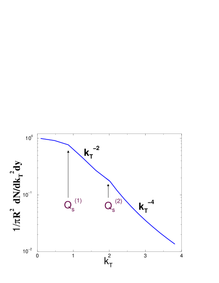
FIG. 2.: Schematic $k_{\perp}$ distribution for particles produced in high-energy $p+A$ collisions (or, more generally, for particles produced in $A_{1}+A_{2}$ collisions at rapidity $y$ such that $\chi_{1}(y)\ll\chi_{2}(y)$). In the perturbative regime, ${\rm d}N/{\rm d}k_{\perp}^{2}{\rm d}y\sim 1/k_{\perp}^{4}$. Inbetween the saturation scales for the two sources, ${\rm d}N/{\rm d}k_{\perp}^{2}{\rm d}y\sim 1/k_{\perp}^{2}$.

A quantitative computation of the radiation distribution requires to determine numerically the CGC density scales $\chi_{1}(y)$ and $\chi_{2}(y)$ from some parametrization of the gluon and quark/antiquark distribution functions. Also, the fragmentation of the radiated gluons into pions must be taken into account. We postpone those issues to a future publication.

From (LABEL:sat_kt2), the $k_{\perp}$-integrated multiplicity in the nonperturbative regime $g^{4}N_{c}\chi_{1}(y)/8\pi\mathrel{\lower 3.87495pt\hbox{$\stackrel{{\scriptstyle\displaystyle<}}{{\sim}}$}}k_{\perp}^{2}\mathrel{\lower 3.87495pt\hbox{$\stackrel{{\scriptstyle\displaystyle<}}{{\sim}}$}}g^{4}N_{c}\chi_{2}(y)/8\pi$ is

$$\frac{{\rm d}N}{{\rm d}^{2}b_{\perp}{\rm d}y}=\frac{1}{4}g^{2}\chi_{1}(y)\frac{N_{c}^{2}-1}{(2\pi)^{2}}\log^{2}\frac{\chi_{2}(y)}{\chi_{1}(y)}~{}.$$ (116)

Thus, at fixed impact parameter, the multiplicity scales as $A_{1}^{1/3}$, up to the square of a logarithm of $(A_{2}/A_{1})^{1/3}$. For the transverse energy in the saturation regime one obtains from (LABEL:sat_kt2)

$$\frac{{\rm d}E_{\perp}}{{\rm d}^{2}b_{\perp}{\rm d}y} = g^{4}\sqrt{\frac{N_{c}}{2\pi}}\frac{N_{c}^{2}-1}{(2\pi)^{2}}\chi_{1}(y)$$ (118)

$$\left(\sqrt{\chi_{1}(y)}-\sqrt{\chi_{2}(y)}+\frac{\sqrt{\chi_{2}(y)}}{2}\log\frac{\chi_{2}(y)}{\chi_{1}(y)}\right)~{}.$$

In the saturation regime (116,118) as well as in the perturbative regime (103,104) the transverse energy per gluon is practically independent of $A_{1}$, while a weak increase $\propto A_{2}^{1/6}$ is expected.

The average transverse momentum in the saturation regime follows from (116,118):

$$\langle k_{\perp}\rangle=2\;Q_{s}^{(2)}\;\frac{\xi-1-\log\xi}{\log^{2}\xi}~{},$$ (119)

where $\xi(y)=\sqrt{\chi_{1}(y)/\chi_{2}(y)}=Q_{s}^{(1)}(y)/Q_{s}^{(2)}(y)$. From dimensional considerations, it has been suggested [13] that in symmetric $A+A$ collisions, and at central rapidity, $\langle k_{\perp}\rangle^{2}$ scales with the multiplicity per unit of transverse area and of rapidity,

$$\langle k_{\perp}\rangle^{2}\propto\frac{{\rm d}N}{{\rm d}^{2}b_{\perp}{\rm d}y}~{}.$$ (120)

A similar scaling relation can be derived from eqs. (116,119) for the asymmetric case,

$$\langle k_{\perp}\rangle^{2}\propto\frac{{\rm d}N}{{\rm d}^{2}b_{\perp}{\rm d}y}\;\frac{g^{2}}{\xi^{2}}\;\frac{\left(\xi-1-\log\xi\right)^{2}}{\log^{6}\xi}~{}.$$ (121)

Thus, $\langle k_{\perp}\rangle^{2}$ is proportional to the multiplicity per unit of rapidity and transverse area, times a function of the ratio of the saturation momenta. If source one is very much weaker than source two, i.e. in the limit $|\log\xi|\gg 1-\xi$, the third factor on the right-hand-side of (121) depends on $\log\xi$ only. Neglecting that dependence, and assuming as before that $\chi_{1,2}$ are proportional to $A_{1,2}^{1/3}$, one has the approximate scaling relation

$$\langle k_{\perp}\rangle^{2}\propto\left(\frac{A_{2}}{A_{1}}\right)^{1/3}\frac{{\rm d}N}{{\rm d}^{2}b_{\perp}{\rm d}y}\propto\left(\frac{1}{A_{1}A_{2}}\right)^{1/3}\frac{{\rm d}N}{{\rm d}y}~{}.$$ (122)

In practice though we expect significant corrections to the simple scaling relation (122), as given by eq. (121).

Qualitatively, the rapidity distribution predicted from eq. (LABEL:sat_kt2) is as follows, see Fig. 3. For rapidities far from the fragmentation region of the large nucleus, and for $g^{4}N_{c}\chi_{1}(y)/8\pi\mathrel{\lower 3.87495pt\hbox{$\stackrel{{\scriptstyle\displaystyle<}}{{\sim}}$}}k_{\perp}^{2}\mathrel{\lower 3.87495pt\hbox{$\stackrel{{\scriptstyle\displaystyle<}}{{\sim}}$}}g^{4}N_{c}\chi_{2}(y)/8\pi$, ${\rm d}N/{\rm d}^{2}k_{\perp}{\rm d}y$ varies like

$$\frac{{\rm d}^{2}N}{{\rm d}y^{2}}\propto g^{2}\chi_{1}^{\prime}(y)~{},$$ (123)

where we have suppressed the dependence on transverse momentum, which is supposed to be held fixed somewhere within the saturation regime. Thus, an experimental measure for the RG evolution of the CGC density parameter is

$$\frac{{\rm d}\log{\rm d}N/{\rm d}y}{{\rm d}y}=\frac{{\rm d}\log\chi_{1}(y)}{{\rm d}y}~{}.$$ (124)

FIG. 3.: Schematic rapidity distribution for particles produced in high-energy $p+A$ collisions (or, more generally, for particles produced in $A_{1}+A_{2}$ collisions at $A_{1}\ll A_{2}$). The upper curve refers to the perturbative regime, the lower curve refers to $k_{\perp}$ between the saturation scales for the two sources.

Now consider the case of high $k_{\perp}^{2}>g^{4}N_{c}\chi_{2}(y)/8\pi$ described by eq. (102). In that regime the rapidity distribution is proportional to $\chi_{1}(y)\chi_{2}(y)$, and so ${\rm d}N/{\rm d}y{\rm d}^{2}k_{\perp}$ varies with rapidity like

$$\frac{{\rm d}\log{\rm d}N/{\rm d}y}{{\rm d}y}=\frac{{\rm d}\log\chi_{1}(y)}{{\rm d}y}+\frac{{\rm d}\log\chi_{2}(y)}{{\rm d}y}~{}.$$ (125)

Subtracting (124) from (125), that is $({\rm d}^{2}N/{\rm d}y^{2})/({\rm d}N/{\rm d}y)$ measured at small transverse momentum from that at larger transverse momentum, provides an experimental measure for the RG evolution of $\chi_{2}(y)$.

IV Summary

In summary, we have computed the radiation field produced in the collision of two ultrarelativistic, non-abelian, classical color charge sources for the case where one of the sources is much stronger than the other. Accordingly, we have linearized the Yang-Mills equations in field 1, but solved them to all orders in field 2. The renormalization-group evolution of the color charge density $\chi$ is not dropped. This problem is relevant for $p+A$ collisions at high energy, or more generally for $A_{1}+A_{2}$ nuclear collisions where $A_{1}\ll A_{2}$, or even for symmetric $A+A$ collisions at large rapidities far away from $y=0$ (i.e. midrapidity) where the RG evolution ensures that the effective $\chi_{1}$ is much smaller than $\chi_{2}$.

We obtain the following results relevant for phenomenology. At high transverse momenta, $k_{\perp}^{2}>g^{4}N_{c}\chi_{2}/8\pi$, the distribution in $k_{\perp}$ is proportional to the standard $\chi_{1}\chi_{2}/k_{\perp}^{4}$ known from perturbation theory. Thus, the unintegrated distribution scales like $(A_{1}A_{2})^{1/3}$. The total contribution from high transverse momenta, integrated over $k_{\perp}$ and impact parameters $b_{\perp}$, scales like $A_{1}^{1/3}A_{2}^{2/3}$.

In the saturation region $g^{4}N_{c}\chi_{2}/8\pi>k_{\perp}^{2}>g^{4}N_{c}\chi_{1}/8\pi$, the distribution is proportional to $\chi_{1}/k_{\perp}^{2}$; it decreases much less quickly with transverse momentum than the result from perturbation theory. This may in principle provide experimental information as to the value of $\chi_{2}(y)$. At fixed $k_{\perp}^{2}$, the gluon distribution scales like $A_{1}^{1/3}$ for fixed impact parameter, or like $A_{1}^{1/3}A_{2}^{2/3}$ when one integrates over ${\rm d}^{2}b_{\perp}$. Note that, up to logarithmic corrections, the $k_{\perp}$-integrated distribution scales in exactly the same way with $A_{2}$ as in the perturbative regime (no matter whether impact parameter selected or integrated). In contrast, at fixed $k_{\perp}$ and $b_{\perp}$ the multiplicity in the perturbative regime scales as $A_{2}^{1/3}$ while in the saturation regime it is independent of $A_{2}$ (up to a logarithm) ! (Or, without impact parameter selection, we have a scaling with $A_{2}$ in the perturbative regime versus scaling with $A_{2}^{2/3}$ in the saturation region.)

Furthermore, at fixed transverse momentum, the quantity ${\rm d}\log({\rm d}N/{\rm d}y)/{\rm d}y$ allows an experimental measurement of the RG evolution of the color charge density parameter $\chi$, and a check whether the saturation regime has been reached. The slope of ${\rm d}N/{\rm d}y$ at rapidities far from the fragmentation region of the large nucleus measures the RG evolution of $\chi_{1}$. Also, subtracting the slope of the ${\rm d}N/{\rm d}y$ measured at small transverse momentum (within the saturation regime) from that at larger transverse momentum (in the perturbative regime), provides experimental access to the RG evolution of $\chi_{2}$, and for its $A$ dependence. Such differential measurements at RHIC and LHC should provide insight regarding high-density QCD and the properties of the CGC, for example the value of its fundamental parameter $\chi$ and its RG evolution (in rapidity).

REFERENCES

• [1] L. McLerran and R. Venugopalan, Phys. Rev. D 49, 2233 (1994); Phys. Rev. D 49, 3352 (1994).
• [2] A. Krasnitz and R. Venugopalan, Nucl. Phys. B 557, 237 (1999); Phys. Rev. Lett.  84, 4309 (2000); Phys. Rev. Lett.  86, 1717 (2001).
• [3] A. Kovner, L. McLerran and H. Weigert, Phys. Rev. D 52, 3809 (1995); Phys. Rev. D 52, 6231 (1995).
• [4] M. Gyulassy and L. McLerran, Phys. Rev. C 56, 2219 (1997).
• [5] Y. V. Kovchegov and D. H. Rischke, Phys. Rev. C 56, 1084 (1997).
• [6] A. H. Mueller, Nucl. Phys. B 558, 285 (1999).
• [7] Y. V. Kovchegov and A. H. Mueller, Nucl. Phys. B 529, 451 (1998); Y. V. Kovchegov, hep-ph/0011252.
• [8] J. Jalilian-Marian, A. Kovner, A. Leonidov and H. Weigert, Phys. Rev. D 59, 014014 (1999); J. Jalilian-Marian, A. Kovner and H. Weigert, Phys. Rev. D 59, 014015 (1999); E. Iancu, A. Leonidov and L. McLerran, hep-ph/0011241; Phys. Lett. B 510, 133 (2001); E. Iancu and L. McLerran, Phys. Lett. B 510, 145 (2001).
• [9] J. Jalilian-Marian, A. Kovner, L. McLerran and H. Weigert, Phys. Rev. D 55, 5414 (1997).
• [10] X. Guo, Phys. Rev. D 59, 094017 (1999).
• [11] I. Balitsky, Nucl. Phys. B 463, 99 (1996); Y. V. Kovchegov, Phys. Rev. D 60, 034008 (1999).
• [12] J. P. Blaizot and A. H. Mueller, Nucl. Phys. B 289, 847 (1987); K. J. Eskola, K. Kajantie, P. V. Ruuskanen and K. Tuominen, Nucl. Phys. B 570, 379 (2000); X. Wang and M. Gyulassy, Phys. Rev. Lett.  86, 3496 (2001); D. Kharzeev and M. Nardi, Phys. Lett. B 507, 121 (2001); H. J. Drescher, M. Hladik, S. Ostapchenko, T. Pierog and K. Werner, hep-ph/0007198; N. Armesto and C. A. Salgado, hep-ph/0011352.
• [13] L. McLerran and J. Schaffner-Bielich, Phys. Lett. B 514, 29 (2001); J. Schaffner-Bielich, D. Kharzeev, L. D. McLerran and R. Venugopalan, nucl-th/0108048.