CP and Flavour
in Effective Type I String Models

Effective type I string models allow stabilization of the dilaton and moduli fields with only a single gaugino condensate. We show that, as well as breaking supersymmetry, the stabilization can spontaneously break CP. We find that this source of CP violation hints strongly at a natural solution to the supersymmetric CP and flavour problems. Even though the CP violation generates physical phases in the Yukawa couplings, all the supersymmetry breaking terms are found to be automatically real and given by the $U(1)$ charges of the associated Yukawa couplings. These can be chosen to have a structure (degenerate or non-universal) which suppresses FCNCs and EDMs. We examine the phenomenological implications, including the generation of the $\mu$-term, and the effect of higher order terms.

Saclay t00/179

1 Introduction

Flavour and CP are especially problematic in supersymmetry because a generic choice of parameters violates experimental bounds on, for instance, $b\rightarrow s\gamma$ and neutron electric dipole moments (EDMs). These two aspects of supersymmetry are known generically as the SUSY flavour and CP problems, and they are probably the most useful tools for probing the underlying theory. In this paper we present a dynamical solution to these problems, which emerges in the light of recent progress on dilaton stabilization in effective models of type I string [1].

Since the importance of dilaton stabilization may be less than transparent, let us begin by discussing the canonical example of a ‘dynamical’ solution to the SUSY flavour and CP problems, dilaton domination. The idea is illustrated schematically in fig.(1a). Supersymmetry breaking is described by the vevs of the auxilliary ($F$) fields. Together they describe a vector whose length is determined by the requirement that the cosmological constant be zero. Its direction however is determined by whatever dynamics breaks supersymmetry. Dilaton domination asserts that it is aligned with the dilaton. Since the dilaton couples equally to all fields, the resulting SUSY breaking terms in the visible sector are very constrained and indeed one finds a suppression of EDMs and FCNCs.

The assumptions underlying dilaton domination are rather more brutal than they might at first appear, since there are more fields than just the dilaton and moduli involved in Planck scale physics. For example, any superfield whose scalar component gets a vev at a high scale can also be involved in transmitting supersymmetry breaking. In particular this is likely to be the case for the very fields that are responsible for flavour structure and CP violation in the first place. Thus one has to assume that, either the spontaneous breaking of CP and flavour does not contribute significantly to supersymmetry breaking thereby affecting the dynamics (e.g. the goldstino angle in the case of dilaton domination), or that the alignment of the goldstino with the dilaton is true a posteriori.

Clearly, a credible ‘dynamical’ solution requires a full determination of the goldstino direction, and that in turn requires a specific model of dilaton and moduli stabilization and spontaneous CP violation. Without all of these ingredients, we think that any dynamical solutions to the SUSY flavour and CP problems will be at best incomplete. To put it more bluntly; can one really trust a dynamical solution to the SUSY CP problem that does not explain the origin of CP violation?

These considerations suggest the approach that we will follow in this paper, which is to avoid tackling flavour and CP head on, but rather to begin by attacking the most difficult part of the problem, namely dilaton stabilization. Our starting point will be the dilaton stabilization scheme found in ref.[1] in effective type I models. As we shall see, this scheme includes a rather generic way to spontaneously break CP. This gives us the required complete dynamical picture of dilaton and moduli vevs, supersymmetry breaking and CP breaking.

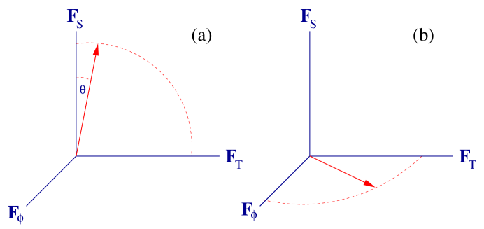
Figure 1: Supersymmetry breaking dynamics leads to non-zero vevs of auxilliary fields of the dilaton, moduli, and any other fields, such as Froggatt-Nielsen fields, that get vevs at high scales. Their relative sizes can be expressed with ‘goldstino’ angles. (a) shows schematically the dilaton domination scenario. (b) shows effective type I models with supersymmetry broken by a condensing D9-brane gauge group, and with stabilized dilaton and moduli fields. The full dynamical calculation relates the $F$-terms and completely determines the goldstino angles.

Anomalous $U(1)$’s play a central role in the stabilization, and consequently the supersymmetry breaking picture which emerges bears some resemblance to the anomalous $U(1)$ mediation models of refs.[2], although the $F$-terms are the dominant source of supersymmetry breaking in the case we examine, rather than the $D$ terms. The picture of supersymmetry breaking that eventually emerges is shown in fig.(1b). The dilaton auxilliary field is zero so supersymmetry breaking is not dilaton dominated. Nevertheless the goldstino direction is determined by the choice of $U(1)$ charges. An appropriate choice gives soft terms that are degenerate providing a leading order suppression of FCNCs that depends only on the charge assignments, and is otherwise independent of the form of Yukawa couplings. In addition, independently of the charge assignments, the soft terms are guaranteed to be real even though the Yukawa couplings can have maximal CP violation, thereby suppressing EDMs. There can, however, be a higher order parametrically small breaking of CP in the soft terms as well. If the CP phase in the CKM matrix happens to be small, this is an explicit manifestation of the approximate CP idea [3].

We stress that we will not make any ad-hoc assumptions about the dilaton or moduli stabilization, or the CP violation which we will treat completely. Moreover, the suppression of FCNCs and EDMs is extremely general, requires no assumptions about the hidden sector particle content and only very mild assumptions about the hidden sector superpotential. Consequently the SUSY breaking in the visible sector can be much more general than the dilaton domination pattern.

We begin in the following section by recapitulating the supergravity scalar potential obtained in ref.[1] and showing how it stabilizes the dilaton and moduli. Here we will discuss the role of modular invariance in the non-perturbative superpotential, and also demonstrate why a similar stabilization mechanism cannot work in the heterotic string. In section III, we present our model for generating Yukawa hierarchies and see how CP can be spontaneously broken. In section IV, we discuss the condensation and string scales allowed by our model. Section V is devoted to the computation of the SUSY breaking terms and we show how CP violation is naturally suppressed in the latter even though it appears in the Yukawa couplings. In section VI we address the problem of the generation of the $\mu$-term and the implications of higher order corrections for the susy flavour and CP problems. We will find that only a mild tuning of couplings can potentially solves these problems. We summarize our results in section VII.

2 Stabilization with and without modular invariance

In this section we discuss the main features of the dilaton stabilization mechanism derived in ref.[1] in the context of effective type IIB orientifold models. We first introduce the effective models, discuss the role of modular invariance in the effective potential, and state the two main assumptions that lead to a stabilization of the dilaton and moduli. We then consider theories both with and without modular invariance. The first case was discussed in ref.[1], and we shall briefly recap the results and generalize them. We then consider models in which the superpotential is constrained by modular symmetries. The modular invariant case has the advantage that the Kähler potential can be adjusted to give a vanishing cosmological constant at the (local) minimum. We also discuss why a similar minimization cannot be achieved in the heterotic string.

2.1 Effective models and modular invariance

Our starting point is the effective theory of $D=4$, $N=1$ type IIB orientifolds. The important features are as follows:

As well as the matter fields, the models contain a complex dilaton $S$, untwisted moduli $T_{i}$ associated with the size and shape of the extra dimensions and complex superfields $M_{k}$ associated with the fixed points (labelled by $k$) of the underlying orbifold. An important property of these models is that the $M_{k}$ superfields appear linearly in the gauge kinetic functions. For gauge groups living on a D9-brane

$$f_{9\,a}=S+\sum_{k}\sigma^{k}_{a}M_{k}\,,$$ (1)

whereas for the D5-branes

$$f_{5_{i}\,a}=T_{i}+\sum_{k}\sigma_{ia}^{k}M_{k}\,,$$ (2)

where $\sigma_{a}^{k}$ are calculable model dependent coefficients and $k$ runs over the different twisted sectors. In most of what follows we will consider only one degenerate value for the $M_{k}$ superfields which we will denote $M$ (it is straightforward to generalize). The $M_{k}$ superfields participate in the generalized Green–Schwarz mechanism for the cancellation of $U(1)_{X}$ anomalies [4]. This contrasts with heterotic models where the dilaton plays this role. Under a $U(1)$ transformation through a phase $\alpha$, the $M_{k}$ fields transform linearly,

$$M_{k}\rightarrow M_{k}+i\frac{\delta_{GS}}{2}\alpha\,.$$ (3)

Type IIB orientifold / heterotic duality has been used to argue that there is also a $\sigma$-model invariance under $SL(2,{\bf Z})$ transformations of the $T_{i}$;

$$T_{i}\rightarrow\frac{a_{i}T_{i}-ib_{i}}{ic_{i}T_{i}+d_{i}}\hskip 8.5359pt;\hskip 14.22636pt\phi_{n}\rightarrow\phi_{n}\prod_{i=1}^{3}(ic_{i}T_{i}+d_{i})^{n_{n}^{i}}\,$$ (4)

where $a_{i},~{}b_{i},~{}c_{i},~{}d_{i}\in{\cal Z}$ and $n_{n}^{i}$ are modular weights of the $\phi_{n}$ with respect to the ith complex direction. These symmetries are broken by the presence of D5-branes, as is obvious from the expressions for $f_{5i}$. However, one expects a remnant of them to survive in directions that are orthogonal to the D5 branes, and again it is the $M_{k}$ fields that shift to cancel any $\sigma$-gauge anomalies [5];

$$M_{k}\rightarrow M_{k}+\sum_{i}\delta^{i}_{k}\ln({ic_{i}T_{i}+d_{i}})\,.$$ (5)

In order to cancel $\sigma-F_{a}$ anomalies, denoted $C_{a}^{i}$, we require

$$\sum_{k}\sigma^{k}_{ia}\delta^{i}_{k}=C_{a}^{i}\,,$$ (6)

for any preserved modular symmetries. The anomalous $U(1)$’s and modular symmetries will be important constraints on the possible form of the superpotential.

When taking into account the presence of $D5$ branes in the vacuum, there are four types of charged matter fields: $C_{i}^{9}$ ($i$ labels the three complex dimensions) comes from open strings starting and ending on the 9-branes; $C_{i}^{5_{j}}$ from open strings starting and ending on the same $5_{i}$-branes; $C^{5_{i}5_{j}}$ from open strings starting and ending on different sets of $5_{i}$-branes; $C^{95_{i}}$ from open strings with one end on the 9-branes and the other end on the $5_{i}$-branes. The Kähler potential for the $S$, $T_{i}$ and $C$ fields is of the general form [7]:

$$K = -\ln\left(S+\overline{S}-\sum_{i}|C_{i}^{5_{i}}|^{2}\right)-\sum_{i}\ln\left(T_{i}+\overline{T}_{i}-|C_{i}^{9}|^{2}-\sum_{j\neq k\neq i=1}^{3}|C_{j}^{5_{k}}|^{2}\right)$$ (7)

$$+\frac{1}{2}\sum_{j\neq k\neq i=1}^{3}\left(\frac{|C^{5_{j}\,5_{k}}|^{2}}{(S+\overline{S})^{1/2}(T_{i}+\overline{T}_{i})^{1/2}}+\frac{|C^{95_{i}}|^{2}}{(T_{j}+\overline{T}_{j})^{1/2}(T_{k}+\overline{T}_{k})^{1/2}}\right)\,.$$

We will only consider $C_{i}^{9}$ because they correspond to the fields which will later condense. $K$ can be rewritten at one loop:

$$K=-\ln\,s-3\ln\tau+\hat{K}(m),$$ (8)

where

$$s=S+\overline{S}\,;\ \ \,\tau=T+\overline{T}-\sum_{n}|\phi_{n}|^{2}\,;\ \ \,m=M+\overline{M}-\delta\ln\tau\,.$$ (9)

We have introduced generic fields $\phi_{n}$ to represent matter fields $C_{i}^{9}$ and for the moment consider only the overall moduli, taking $T_{i}=T$, $M_{k}=M$ and $\delta^{i}_{k}=\delta$ leaving the more general case for later. We shall express all quantities including the string scale ($M_{s}$) in natural units where $M_{P}=1$ and for later convenience define fields scaled in string units with a tilde – for example $\tilde{\phi}=\phi/M_{s}$. The first two terms have the usual “no-scale” structure with the $T$ and $\phi_{n}$-dependence appearing in the combination $\tau$ only. All $M$ dependence appears in the modular invariant combination, $m$, and giving a vev to $m$ takes us away from the orientifold point. The $\delta\ln\tau$ correction can be deduced from the one loop expression for the gauge coupling and depends on the tree-level expression for $K$. Although it is currently unclear what the precise form of the $m$-dependence in the Kähler potential should be, we know that $\hat{K}$ is an even function of $m$ thanks to the orbifold symmetry, and that the leading term in an expansion about the orientifold point, $m=0$, is quadratic, $\hat{K}=\frac{1}{2}m^{2}+\ldots$. We will accommodate the uncertainty in the form of $\hat{K}$ by working with the parameter $x=\partial\hat{K}/\partial M$ where near the orientifold point $x\approx m$.

2.2 Two assumptions for stabilization

This completes the general overview of the type I models that will form the basis for our discussion. In order to stabilize the dilaton, we now augment them with two mild assumptions about the superpotential:

• Our first assumption is that there is a non-perturbative contribution to the superpotential, $W_{np}$, which is generated by hidden sector gaugino condensation with single gauge group $SU(N_{c})$ residing on a D9-brane and with extra (anti)quarks ($\overline{{\cal Q}}$) ${\cal Q}$ in the (anti)fundamental representation of $SU(N_{c})$. Below the scale $\Lambda=M_{s}e^{-f_{9}/2\beta}$, where $\beta=\frac{3N_{c}-1}{16\pi^{2}}$, $\overline{{\cal Q}}$ and ${\cal Q}$ form a composite meson field, $\phi_{0}=\sqrt{{\cal Q}\overline{\cal Q}}$. $W_{np}$ is fixed uniquely by global symmetries and reads

  $$W_{np}=\left(\frac{\Lambda^{3N_{c}-1}}{\phi_{0}^{2}}\right)^{\frac{1}{N_{c}-1}}\,.$$ (10)

  There is no $T$-dependence in this expression since there is no $T$-dependence in the one-loop expression for the gauge kinetic function $f_{9}$ in the type I case. Note that the superpotential is also invariant under the $U(1)_{X}$ symmetry, and has the correct modular behaviour. For example, the lagrangian is invariant under overall modular transformations if the combination $G=K+\ln|W|^{2}$ is invariant, which implies that $W_{np}$ has weight $-3$. In models where there are no D5-branes, this is the case and the necessary modular weight is provided by $\phi_{0}$ and the transformation of $M$; $Z_{3}$ and $Z_{7}$ orientifolds have $f_{9}=S\pm\beta M$ with our definitions, and under an $SL(2,{\cal Z})$ transformation $M\rightarrow M\pm 2\ln({icT+d})$ [5]. Thus both $\Lambda$ and $\phi_{0}$ have weight $-1$, and $W_{np}$ has overall weight $-3$ as required. This is also true when there are $N_{m}$ mesons, in which case it is det$(\tilde{\cal Q}{\cal Q})$ (with weight $-2N_{m}$) that appears in the denominator. As we mentioned above, the $T_{i}$ modular symmetries are broken by the presence of D$5_{i}$-branes, but are expected to be preserved along the directions without them.

• The second assumption is that, as well as the MSSM, the superpotential contains additional pieces involving the remaining fields $\phi_{m=1,..N}$. In particular the extra terms should generate a perturbative mass term for $\phi_{0}$ (e.g. $\phi_{1}\phi_{0}^{2}$). The $\phi_{m}$ and $\phi_{0}$ are charged under the anomalous $U(1)_{X}$ with charges $q_{m,0}$, so that the perturbative piece of the hidden sector superpotential can always be written in terms of the $m$ invariants of $U(1)_{X}$ which we can choose arbitrarily to be $X_{m}={\phi}_{m}^{-2q_{0}/q_{m}}{\phi}_{0}^{2}$.

2.3 The general form of the scalar potential

In type I models, the Kähler metric can be inverted without approximation, and the resulting scalar potential takes the form [1]

$$V_{F}=e^{G}B\,,$$ (11)

where

$$G = K+\ln|W|^{2}\,$$

$$B = \delta B_{0}+\left|1-s\frac{W_{S}}{W}\right|^{2}+\frac{\tau}{(3+\delta x)}\sum_{n}\left|\frac{W_{n}}{W}\right|^{2}+\hat{A}\left|B_{0}+\sigma\frac{W_{S}}{W}\right|^{2}$$

$$B_{0} = x-\frac{\delta}{\hat{A}}$$

$$\hat{A} = \frac{1}{\hat{K}_{M\overline{M}}}+\frac{\delta^{2}}{3+\delta x}\,,$$ (12)

and where subscripts denote differentiation, and it is convenient to define $x=K_{M}$. The potential can be expressed more concisely in terms of the auxilliary fields,

$$F^{\alpha}=e^{-G/2}G^{\alpha\overline{\beta}}G_{\overline{\beta}}\,.$$ (13)

The $F$-terms that we need are

$$F^{S} = e^{G/2}\,.s\left(s\frac{\overline{W}_{S}}{\overline{W}}-1\right)$$

$$F^{M} = e^{G/2}\,.\hat{A}\left(B_{0}+\sigma\frac{\overline{W}_{S}}{\overline{W}}\right)$$

$$F^{0} = \phi_{0}e^{G/2}\,.\frac{1}{|\hat{\phi}_{0}|^{2}}\left(2\sum_{m}\frac{X_{m}\overline{W}_{X_{m}}}{\overline{W}}+\frac{1}{4\pi^{2}}\frac{\overline{W}_{S}}{\overline{W}}\right)$$

$$F^{m} = \phi_{m}e^{G/2}\,.\frac{-2q_{0}}{q_{m}|\hat{\phi}_{m}|^{2}}\frac{X_{m}\overline{W}_{X_{m}}}{\overline{W}}\,.$$ (14)

Above and henceforth, we denote canonically normalized fields with a hat;

$$\hat{\phi}_{n}=\sqrt{\frac{\mbox{$(3+\delta x)$}}{\tau}}\phi_{n}\,\,;\,\,\hat{F}^{n}=\sqrt{\frac{\mbox{$(3+\delta x)$}}{\tau}}F^{n}\,\,;\,\,\hat{F}^{S}=\frac{1}{s}F^{S}\,\,;\,\,\hat{F}^{M}=\frac{F^{M}}{\sqrt{\hat{A}}}\,.$$ (15)

In terms of the canonically normalized auxilliary fields we have

$$V_{F}=e^{G}\delta B_{0}+|\hat{F}^{S}|^{2}+|\hat{F}^{M}|^{2}+\sum_{n=0}|\hat{F}^{n}|^{2}\,.$$ (16)

This form is reminiscent of the no-scale models, however the potential is not positive definite since the functions $B_{0}$ can be negative for finite values of $x$. Indeed, when $\hat{F}^{S,M,n}=0$, supersymmetry is restored where $3+\delta x=0$. Here we find the global minimum with $V_{F}=-3e^{G}$.

In addition to the $F$-term contribution, there is an important $D$-term contribution coming from the anomalous $U(1)$, which takes the form

$$V_{D}=\frac{g_{X}^{2}}{2}D_{X}^{2}\,,$$ (17)

where

$$D_{X}=q_{n}|\hat{\phi}_{n}|^{2}-\delta_{GS}\frac{x}{2}\,.$$ (18)

The Fayet–Iliopoulos term,

$$\xi^{2}=\frac{1}{2}\delta_{GS}x\,,$$ (19)

is given by $m$ as opposed to $S$ and so can be zero [5, 10].

Before tackling the stabilization in detail, let us first highlight the general features of the potential that make it possible. The important aspect of the $V_{F}$ contribution to the potential is that $W_{S}/W$ appears twice, both in $\hat{F}^{M}$ and $\hat{F}^{S}$, due to the $M$ contribution to the gauge kinetic function. In previous work, the assumption has usually been that integrating out the mesons leads to $W\sim e^{-8\pi^{2}S/\beta}$ so that $W_{S}/W$ inevitably ends up being a negative constant. In the present type I case however, we leave $W_{S}/W$ as a fully dynamical variable and, by employing an additional perturbative contribution to the superpotential, set its vev to be positive thanks to the $F^{M}$ contribution. The dilaton then trivially finds its minimum where $\hat{F}^{S}=0$. The $D$-term contribution is important because it forces a local minimum at a finite value of $x$, where supersymmetry is broken. There is thus an interesting interplay between the $F$ and $D$-term contributions.

2.4 Stabilization without modular invariance

In ref.[1] it was shown that our two assumptions can lead to a natural stabilization of the dilaton. In that example, which we shall now briefly recap, the superpotential is of the form

$$W=W_{np}+W_{p}\,,$$ (20)

where the perturbative part of the superpotential, $W_{p}(X_{m})$, is some function of gauge invariants.

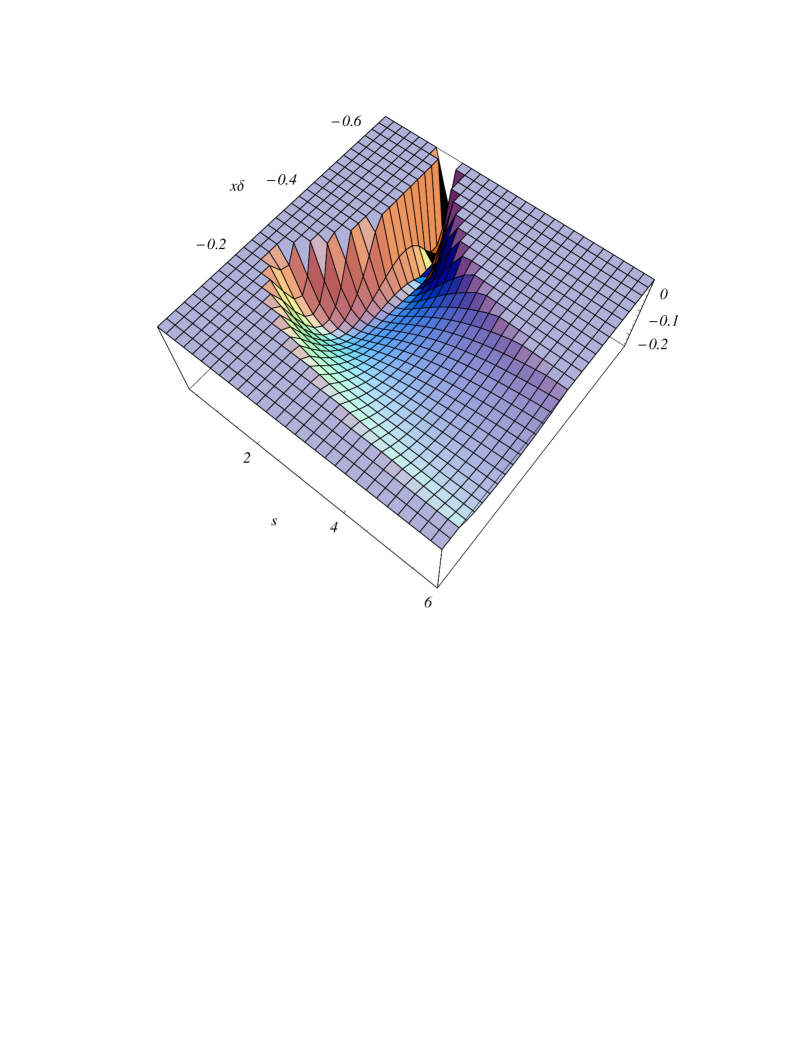
Figure 2: The $F$-part of the potential (11) in the plane ($s,x$) where $s=S+\overline{S}$ and $x=\frac{\partial{\hat{K}}}{\partial M}\sim m$ at small $m$. The valley approaches $x=0$ at large dilaton values. Thus, starting at the orientifold point $m=0$, the field can roll down this valley from large $s$ values to its minimum.

Let us first assume that $x=K_{M}$ has a non-zero value and determine the corresponding vevs of all the other fields. This will lead to a potential purely in $x$, whose minimization we shall consider at the end. The $D$-term clearly dominates the potential in any reasonable model (with $e^{G}\sim m_{W}^{2}$), so we begin the minimization by as usual imposing $D_{X}=0$;

$$\sum_{n}q_{n}|\hat{\phi}_{n}|^{2}=\frac{|\delta_{GS}x|}{2}\,,$$ (21)

where we have anticipated that $\langle\delta_{GS}x\rangle$ will eventually be positive. This equation determines $\tau$ in terms of the other fields, since it does not appear elsewhere in the potential. For definiteness we will take $q_{0}>0$.

The minimization of $V_{F}$ is equivalent to minimizing $B$ if the final cosmological constant is small or zero as we must check at the end. The independent variables are $s$, $\phi_{m>0}$ and $\phi_{0}$, but things simplify greatly if we can trade them; $\phi_{m}$ for $X_{m}$, and $\phi_{0}$ for $W_{S}/W$. We can do this if, defining

$$\rho_{m}=\frac{q_{m}|\phi_{m}|^{2}}{q_{0}|\phi_{0}|^{2}}\,,$$ (22)

the solutions satisfy $\rho_{m}\ll 1$. We shall see shortly how this can be achieved.

Minimization under this approximation gives simple but non-trivial relations between the auxilliary fields;

$$F^{0} = \frac{q_{0}\phi_{0}}{q_{m}\phi_{m}}F^{m}=-4\pi^{2}\sigma\phi_{0}F^{M}=\frac{e^{G/2}}{s}\frac{q_{0}\phi_{0}}{2\pi^{2}|\delta_{GS}.x|}$$

$$F^{S} = 0\,,$$ (23)

to leading order in $\rho_{m}$. These dynamical relations will be important in determining the behaviour of the soft terms. In particular they ensure nice properties such as reality of $A$-terms. Note that without $W_{np}$ the minimizations separate and we trivially find $F_{n}=0$. Thus supersymmetry is always unbroken before condensation.

The resulting expression for the stabilized dilaton is

$$s(x)=-\frac{\sigma^{2}+\lambda^{2}}{\sigma B_{0}}+{\cal O}(\rho_{m})\,,$$ (24)

where we have defined

$$\lambda^{2} = \frac{1}{\hat{A}}.\frac{q_{0}}{8\pi^{4}|\delta_{GS}x|}\,.$$ (25)

The remaining equations, determining the vevs of $\phi_{0}$ and $\phi_{m}$ respectively, can be written in terms of $s(x)$;

$$\frac{W_{S}}{W} = \frac{1}{s}$$

$$X_{m}\frac{W_{X_{m}}}{W} = \frac{q_{m}\rho_{m}}{q_{0}8\pi^{2}s}+{\cal O}(\rho_{m}^{2})\,.$$ (26)

The first requirement for this solution, and our assumption, to be consistent, is that the perturbative superpotential has couplings such that $\partial W_{p}/\partial X_{m}\approx 0$ gives $\mbox{$\langle W_{p}\rangle$}\neq 0$, and the assumed $\rho_{m}\ll 1$. The second requirement is of course that $s$ is positive (and hence that $B_{0}(x)/\sigma$ is negative) for the particular value of $x$.

On examining the remaining $x$-dependent potential, we find that a minimum can develop where all of these conditions are satisfied; assuming that we have chosen parameters such that $\rho_{m}\ll 1$, the potential is given by

$$B=B_{0}\frac{\delta}{\sigma^{2}+\lambda^{2}}\left(\sigma^{2}-\sigma_{0}^{2}\right)\,,$$ (27)

where $\sigma_{0}^{2}$ is a constant; $\sigma_{0}^{2}=\frac{q_{0}}{8\pi^{4}\delta_{GS}\delta}$. Two options can now be considered for determining the value of $x$;

• The no-scale option: Set the cosmological constant to be exactly zero. As we have seen, $\sigma B_{0}$ must be non-zero and negative to stabilize the dilaton. However we can make the potential completely flat by choosing $\sigma=\sigma_{0}$. The $x$ dependent vevs for $\phi_{m}$, $\phi_{0}$, $\tau$ and $s$ then correspond to a flat direction with zero cosmological constant. A natural possibility is that $x$ and therefore $M$ can be fixed by minimizing the potential after radiatively induced electroweak symmetry breaking.

• The Kähler stabilization option: particular forms of $\hat{K}$ can give a local minimum in the function $B_{0}(x)$ with a small but negative cosmological constant of order $-\delta^{2}$. The minimization condition is found to be

  $$\delta\frac{\partial K_{M\overline{M}}}{\partial x}=1+\frac{2\delta^{2}K_{M\overline{M}}}{3+\delta x}\,.$$ (28)

  For example when

  $$\hat{K}(m)=\frac{3}{a}\ln\left(1+\frac{a}{6}m^{2}\right)\,,$$ (29)

  the minimum in $\delta B_{0}$ is at $\delta x<0$, and gives a cosmological constant

  $$\delta B_{0}|_{min}\approx\frac{1}{2a}-\delta^{2}.$$ (30)

  In conjunction with the $D=0$ condition, this implies that $\delta_{GS}\delta q_{0}>0$. The dilaton vev is

  $$s\approx\frac{\sigma}{\delta^{2}}\,,$$ (31)

  so that we require negative $\sigma$. The potential in this case is shown in fig.2 where we have eliminated $\tau$ and $\phi_{n}$ and show the dependence on $s$ and $x$ for $K_{M\overline{M}}=e^{-60x^{2}}$. In particular (as an aside) note that there is no barrier between large dilaton values and the minimum. This contrasts with the multiple gaugino condensate scenario, which has a barrier and hence an ‘initial value’ problem for the dilaton. Finally, note that the imaginary axionic components of $S$, $T$ and $M$ are not fixed by the above but will be fixed separately by the Peccei-Quinn mechanism.

We repeat that the remaining fields ($S,~{}T,~{}\phi_{0}$) are all fixed as long as $x$ is fixed by one of the above mechanisms. The virtue of this set-up is therefore that the problem of dilaton/moduli stabilization is reduced to stabilizing one of the blowing up modes at a non-zero value. The $m$ dependence in the Kähler potential which brings this about is unknown, however the set of dynamical relations between the auxilliary fields is already very restrictive and, as we shall see in section 5, hints strongly at a solution to the SUSY flavour and CP problems.

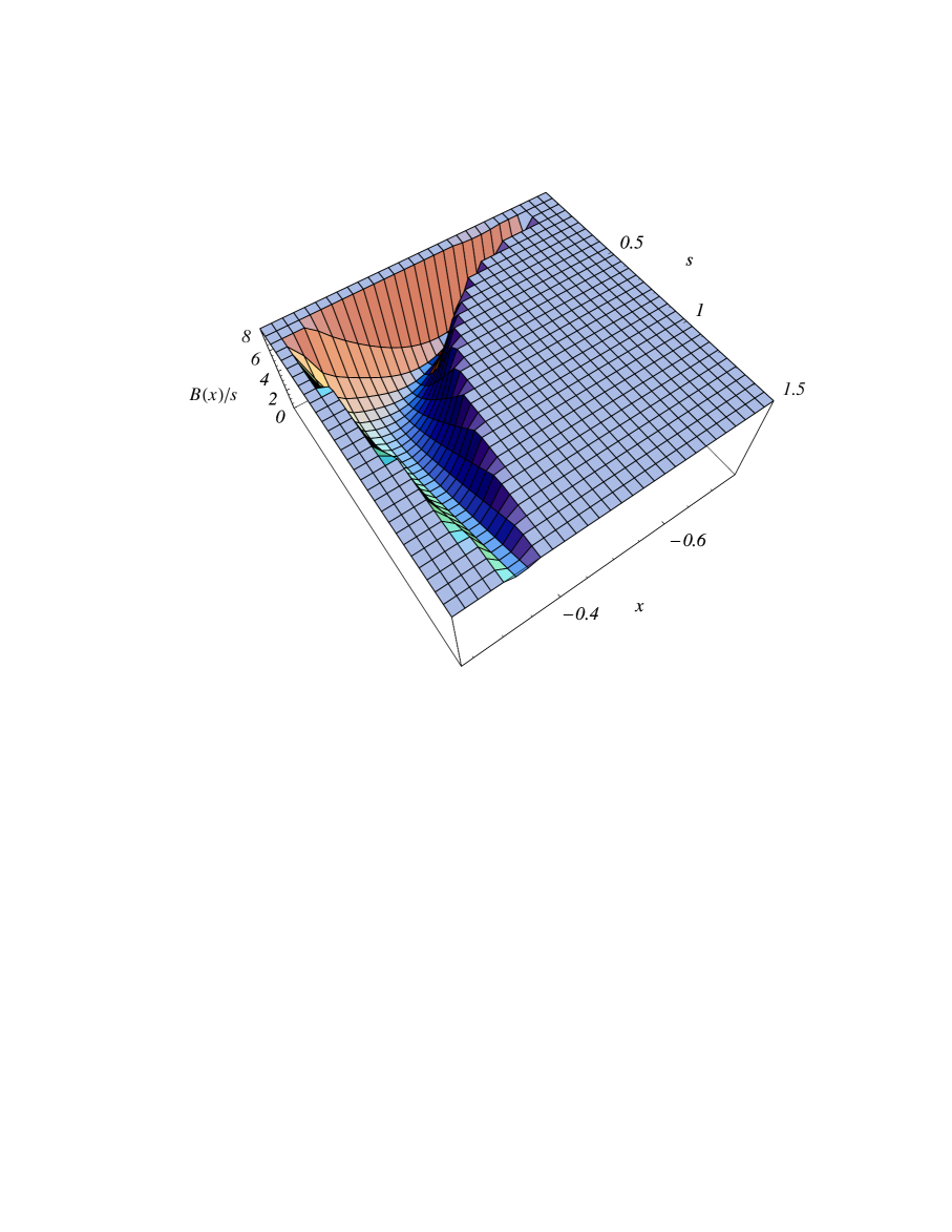
Figure 3: The $F$-part of the potential (11) for the modular invariant case in the plane ($s,x$), where $s=S+\overline{S}$ and $x=\frac{\partial{\hat{K}}}{\partial M}\sim m$. The local minimum has zero cosmological constant. The global supersymmetric minimum is now located outside the diagram towards its top left (it was on the top right of the previous graph).

2.5 Stabilization with modular invariance

The stabilization above is quite appealing, but an important aspect is that $W_{p}$ necessarily breaks any modular invariance if $\langle W_{p}\rangle$ is to be non-zero. One might therefore wonder how general this mechanism is, and in particular, if it can work in models that retain some or all of the initial modular invariance. In this subsection we shall show that this is indeed the case. In such models, the superpotential is necessarily very different from that in eq.(20), however the same stabilization mechanism can be employed.

In order to include modular invariance, let us return to the superpotential, which is now required to have the correct weight. We will consider the case of invariance under overall modular transformations (involving $T$), for which the non-perturbative contribution $W_{np}$ in eq.(10) has to have weight -3. This is the case if the GS terms obey

$$\delta\sigma=-2\beta\,.$$ (32)

In addition $U(1)_{X}$ invariance of $W_{np}$ requires

$$\delta_{GS}\sigma=\frac{q_{0}}{2\pi^{2}}\,.$$ (33)

As we saw, both of these relations are obeyed in $Z_{3}$ and $Z_{7}$ orientifold models.

To construct the rest of the superpotential, we begin by forming gauge and modular invariant (and dimensionless) combinations of fields using the appropriate power of $W_{np}$. These we shall denote $\tilde{X}_{m}$;

$$\tilde{X}_{m}=\frac{X_{m}}{M_{s}^{2(1-q_{0}/q_{m})}}\left(\frac{W_{np}}{M_{s}^{3}}\right)^{({2q_{0}-2q_{m}})/{3q_{m}}}\,.$$ (34)

We can now write the most general expression for the superpotential as

$$W=W_{np}\times f(\tilde{X}_{m})\,,$$ (35)

where $f$ is any function of the invariants. The most trivial possibility with only one invariant, $\tilde{X}$, is $f=1+\tilde{X}$ in which case the superpotential is again just the sum of a nonperturbative and perturbative part

$$W=W_{p}+W_{np}.$$ (36)

(We can of course express any perturbative contribution in terms of $\tilde{X}_{m}$; for example $\phi_{2}\phi_{0}^{2}+\phi_{2}\phi^{2}_{1}=W_{np}(\tilde{X}_{2}+\tilde{X}_{2}/\tilde{X}_{1})$ and so on.) However in what follows, and in particular in order to spontaneously break CP, we will leave the expressions in the general form of eq.(35).

The imposition of modular invariance has removed one of our degrees of freedom since a priori eq.(35) gives

$$\frac{W_{S}}{W}=-\frac{8\pi^{2}}{N_{c}-1}\left(1+\sum_{m=1}\frac{2}{3}\frac{\tilde{X}_{m}f_{m}}{f}\left(\frac{q_{0}}{q_{m}}-1\right)\right)\,.$$ (37)

Therefore, the simplest case we can consider now has $\phi_{0}$ plus one other field (which we shall take to be $\phi_{1}$) getting large vevs. If this is the case, we can eliminate $\hat{\phi_{0}}$ using the $D$-term constraint, and then minimize in $s$, $\hat{\phi}_{1}$ and $\tilde{X}_{m}$ independently. These minimizations again relate the vevs of the auxilliary fields;

$${F^{1}} = \frac{1}{p}\frac{\phi_{0}}{\phi_{1}}{F^{0}}$$

$$F^{M} = -\frac{F^{0}}{8\pi^{2}\sigma\phi_{0}}\frac{3N_{c}-1+2p}{1+p}$$

$$F^{S} = 0$$

$$F^{m>1} = 0\,,$$ (38)

where $p=\pm\sqrt{q_{0}/q_{1}}$, upto corrections of order $\rho_{m>1}$. In order for these relations to be consistent, the charge $q_{1}$ must have the same sign as $q_{0}$, and again we must check later on that we end up with $\mbox{$\langle W_{S}/W\rangle$}>0$. Eqs.(2.5a,b) imply that $F^{\rho}\partial_{\rho}g(\tilde{X}_{1})=0$ for any function $g(\tilde{X}_{1})$. As in the non-modular invariant case, this will give nice phenomenological properties such as reality of $A$-terms.

Note that summing the last two equations and using $F_{S}=0$ gives the constraint in eq.(37). Inserting these solutions back into $V_{F}$, we now find the $x$ dependent potential to be

$$B=B_{0}\frac{\delta}{\sigma^{2}+\lambda^{2}}\left(\sigma^{2}-\sigma_{0}^{2}+\frac{2C_{0}\sigma_{0}^{2}}{x}-\frac{C_{0}^{2}\sigma_{0}^{2}}{xB_{0}(x)}\right)\,,$$ (39)

where now

$$\sigma_{0}^{2} = \frac{q_{0}}{32\pi^{4}\delta_{GS}\delta}\frac{(3N_{c}-1+2p)^{2}}{(1+p)^{2}}$$ (40)

$$= \sigma^{2}\frac{(3N_{c}-1+2p)^{2}}{{(1+p)^{2}}{(3N_{c}-1)}}\,.$$

The resulting expression for the stabilized dilaton is

$$s(x)=-\frac{\sigma^{2}+\lambda^{2}}{\sigma B_{0}+{\lambda^{2}}C_{0}}+{\cal O}(\rho_{m>1})\,,$$ (41)

where we have defined

$$\lambda^{2} = \frac{1}{\hat{A}}.\frac{q_{0}}{32\pi^{4}|\delta_{GS}x|}\frac{(3N_{c}-1+2p)^{2}}{(1+p)^{2}}$$

$$C_{0} = \frac{24\pi^{2}}{3N_{c}-1+2p}.$$ (42)

The remaining equations can again be written in terms of $s(x)$;

$$\frac{1}{\rho_{1}} = \frac{2(p^{2}-1)}{3p(8\pi^{2}s+N_{c}-1)}-\frac{1}{p}$$

$$X_{1}\frac{f_{X_{1}}}{f} = \frac{3}{2(p^{2}-1)}\left(1+\frac{N_{c}-1}{8\pi^{2}s}\right)$$

$$X_{m>1}\frac{f_{X_{m}}}{f} = 0\,.$$ (43)

The minimization of this potential is rather more involved than that of the previous subsection, and we have to be careful to ensure that both $s$ and $K_{M\overline{M}}$ are positive, and also that $K_{M\overline{M}}(0)=1$. We have identified four possibilities;

• Minimization with a large positive cosmological constant; this happens quite readily for arbitrary $M$ dependence in the Kähler potential, due to the $1/x$ terms in eq.(39).

• Minimization at $s=\infty$ corresponding to $V_{F}=0$.

• The no-scale option; in this case we now have to tune away the $1/x$ dependence in eq.(39) and the cosmological constant. The simplest way to do this is to set $\sigma^{2}-\sigma^{2}_{0}=\sigma^{2}_{0}(2C_{0}-C_{0}^{2}/B_{0})/x$ and then work backwards to find the required function $K_{M\overline{M}}(x)$. Note that $\sigma_{0}=\sigma$ is satisfied for $\frac{q_{0}}{q_{1}}=\frac{3N_{c}-1}{2}$, however this choice leads to negative $s$.

• A minimum in $x$ at zero cosmological constant; the simplest way to find these is to ‘perturb’ away from a no-scale solution.

An example of the 4th case is shown in fig.3 where we plot $B/s$ with all fields eliminated except $x$ and $s$. In this rather simplified case (with only one meson and one additional field) imposing a zero cosmological constant forces rather extreme choices of parameters in order to get a minimum at small $x$; in the example shown we have taken $q=1/3,~{}\delta=7.6,~{}N_{c}=5$ and $p=-3.4$. (The remaining parameters $\sigma$ and $\delta_{GS}$ are fixed by eq.(32) and (33).) The form of the potential is similar to that in fig.2, however passing over the barrier and continuing to large $x$ takes us to the no-scale case, and unbroken supersymmetry is now found at smaller (but finite) value of $x$. In addition, there is now a barrier between this minimum and the orbifold point. The minimum is at $\frac{d{B_{0}}}{dx}\approx 0$ as previously, so that eq.(28) still applies.

2.6 Relation to the heterotic string

To complete this discussion we should relate this stabilization picture to that in heterotic strings where dilaton stabilization appears to be much more difficult. In particular, in the heterotic case the gauge kinetic function at one loop goes like $f_{a}=k_{a}S-\frac{3}{8\pi^{2}}c_{a}\ln\eta(T)^{2}$ where $T$ is again the overall modulus, $c_{a}$ is determined by a string computation and $\eta(T)=e^{-\pi T/{12}}\prod_{n=1}(1-e^{-2\pi nT})$ is the Dedekind $\eta$ function. At large values of $T$, $\eta(T)\sim e^{-{\pi T}/{12}}$ so that $f_{a}\sim k_{a}S+\frac{3c_{a}}{48\pi}T$ and one might wonder why a stabilization is not possible in this case as well, simply by replacing $M$ with $T$.

There are two reasons. The first is the different form of the Kähler potential. In the present case the leading term goes as $m^{2}=(M+\overline{M})^{2}$ as opposed to $-3\log(T+\overline{T})$ in the heterotic case. Thus in the scalar potential we have $K_{M}\sim m$ tending to stabilize $\langle m\rangle$ at small values, as opposed to the heterotic case which has $K_{T}\sim-\frac{1}{T+\overline{T}}$ tending to push $\langle T\rangle$ to large values. The type I stabilization therefore occurs only where $\langle m\rangle$ is small, of order $\delta$, and in this region the above approximation does not hold.

The second reason is that the stabilization relies heavily on the presence in the potential of anomalous $U(1)$ $D$-terms. In type I strings these contain a Fayet-Iliopoulos term that is proportional to $m$. Thus equating $m$ in type I with $T+\overline{T}$ in the heterotic string, would require the heterotic Fayet-Iliopoulos term to go like $\sim(T+\overline{T})$ rather than $1/(S+\overline{S})$ as is actually the case.

3 Generating CP and flavour structure in Yukawas

In the previous section we saw how dilaton and moduli stabilization can occur in type I models assuming a single condensing gauge group and an anomalous $U(1)$. In following sections we shall show that the distribution of supersymmetry breaking amongst the different fields is such that SUSY contributions to flavour and CP violating processes are naturally suppressed. First however, we need a working model of flavour and CP violation.

The possibilities for generating flavour structure are restricted, since our guiding principle is to determine all contributions to SUSY breaking, and hence all the goldstino angles. So, we cannot simply insert an additional Froggatt-Nielsen field without going back to consider the additional contribution to SUSY breaking when it gets a VEV. Our Froggatt-Nielsen fields can therefore only be the $\phi_{n}$, and we will henceforth assume that it is these fields that play a role in generating Yukawa hierarchies by getting vacuum expectation values.

There are many ways in which the required flavour structure could arise, but in order to have a working example, consider the case with only one extra field $\phi_{1}$ with charge $2q_{1}=-q_{0}$, so that we have just one relevant invariant $X=\phi_{1}\phi_{0}^{2}\,.$ In the case without modular invariance, the most general form of Yukawa coupling can be written

$$Y_{\alpha\beta\gamma}=\tilde{\phi_{0}}^{q_{\alpha\beta\gamma}/q_{0}}g_{\alpha\beta\gamma}({\tilde{X}})$$ (44)

where $q_{\alpha\beta\gamma}$ is the $U(1)$ charge of the Yukawa coupling, and $g_{\alpha\beta\gamma}$ is any function of $\tilde{X}$. In eq.(44), for the case without modular invariance, the tilde’s imply multiplication by powers of $M_{s}$ to make dimensionless quantities.

We will see in the following sections that suppression of SUSY flavour-changing processes depends on choosing degenerate charges. We therefore propose that the $U(1)$ charges of the first and second generation charges are degenerate since these generations give rise to the most restrictive flavour changing processes. If $|\mbox{$\langle\tilde{X}\rangle$}|\ll 1$, we can choose charges such that the Yukawa couplings take the form

$$Y_{U_{ij}}\mbox{$\langle h_{2}^{0}\rangle$}\approx\left(\begin{array}[]{ccc}m_{c}&m_{c}&0\\ m_{c}&m_{c}&0\\ 0&0&m_{t}\end{array}\right)+{\cal O}(m_{t}\tilde{X}+\ldots)\,,$$

and similar for down and lepton Yukawas, where $m_{c}$ and $m_{t}$ are functions of $\phi_{0}$ only. For the canonically normalized top quark, we find a mass term

$$\hat{m}_{t}=\mbox{$\langle h_{2}^{0}\rangle$}{\tilde{\phi}_{0}^{-(q_{H_{2}}+q_{t_{L}}+q_{t_{R}})/q_{0}}}{\sqrt{\tau^{n_{H_{2}}+n_{t_{L}}+n_{t_{R}}}}}\,,$$ (45)

where $n_{\alpha}$ are the weights of the fields. The $D$-term constraint imposes $|\phi_{0}^{2}|\sim|\delta_{GS}x|\tau M_{P}^{2}$ so that we can rewrite the top mass as

$$\mbox{$\langle h_{2}^{0}\rangle$}\sqrt{|\delta_{GS}x|^{-(q_{H_{2}}+q_{t_{L}}+q_{t_{R}})/q_{0}}}{\sqrt{\tau^{n_{H_{2}}+n_{t_{L}}+n_{t_{R}}-(q_{H_{2}}+q_{t_{L}}+q_{t_{R}})/q_{0}}}}\left(\frac{M_{P}}{M_{s}}\right)^{-(n_{H_{2}}+n_{t_{L}}+n_{t_{R}})}$$ (46)

In order to avoid very large values (coming from a large $\langle\tau\rangle$) we impose

$$n_{H_{2}}+n_{t_{L}}+n_{t_{R}}=\frac{q_{H_{2}}+q_{t_{L}}+q_{t_{R}}}{q_{0}}\,,$$ (47)

and in order to have a large top mass we require $(q_{H_{2}}+q_{t_{L}}+q_{t_{R}})/q_{0}\approx 0$. Imposing also that $n_{H_{2}}+n_{c_{L}}+n_{c_{R}}=(q_{H_{2}}+q_{c_{L}}+q_{c_{R}})/q_{0}$, we find that

$$\hat{m}_{c}=\hat{m}_{t}\sqrt{|\delta_{GS}x|^{(q_{t_{L}}+q_{t_{R}}-q_{c_{L}}-q_{c_{R}})/q_{0}}}\left(\frac{M_{P}}{M_{s}}\right)^{n_{t_{L}}-n_{c_{L}}+n_{t_{R}}-n_{c_{R}}}$$ (48)

At leading order the Yukawa couplings have an accidental U(2) symmetry and hence a zero eigenvalue. The higher order terms in $\tilde{X}$ will generally break this symmetry and give masses to the first generation. Thus, we require

$$|\mbox{$\langle\tilde{X}\rangle$}|\sim\frac{m_{u}}{m_{t}}\,.$$ (49)

Such values of $|\mbox{$\langle\tilde{X}\rangle$}|$, and also CP violating phases of order 1, can quite easily be generated during the minimization. The $\tilde{X}$ dependent perturbative part of the superpotential can be any function of $\tilde{X}$ but as a rather trivial example consider the case without modular invariance, with

$$W_{p}=(a\tilde{X}+\frac{b}{2}\tilde{X}^{2}+\frac{c}{3}\tilde{X}^{3})M_{s}^{3}\,.$$ (50)

In this expression we assume that non-renormalizable interactions between the fields are suppressed by powers of $M_{s}$ so that (since $\tilde{X}=X/M_{s}^{3}$) $a,b,c$ are of order one. Recall that our approximations required $|\phi_{1}|\ll|\phi_{0}|$ so that, as we saw above, the minimum is close to $\partial W_{p}/\partial\tilde{X}=0$. The $D$-term constraint imposes $|\phi_{0}^{2}|\sim|\delta_{GS}x|\tau$ and so provided $\tau\gg|\delta_{GS}x|^{-1}$ (which is the case) we can check that, for the desired value of $\tilde{X}$, this approximation is good. It is now trivial to choose couplings to give the desired $\mbox{$\langle\tilde{X}\rangle$}\sim m_{u}/m_{t}$.

The physically observable CP violation depends only on the phase of $\tilde{X}$. To see this, suppose for example that the explicit form of the Yukawa couplings is

$$\left(\frac{\langle\phi_{0}\rangle}{M_{s}}\right)^{n_{ij}}H_{2}{Q_{i}}U^{c}_{j}\ +\ \left(\frac{\langle\phi_{1}\rangle}{M_{s}}\right)^{n_{kl}}H_{1}{Q_{k}}D_{l}^{c}\,.$$ (51)

One of the phases can always be $R$-rotated away, and the remaining phase, $\theta=(\theta_{1}-\frac{q_{1}}{q_{0}}\theta_{0})$, is nothing other than the phase of $X$. (In general one needs at least two Froggatt–Nielsen fields to generate CP violation.) Therefore, generating a physically measurable spontaneous breaking of CP in the Yukawa couplings is equivalent to giving a phase to the gauge invariant $X$, i.e. by choosing $b^{2}-4ac<0$.

A similar situation applies in the modular invariant case. Explicitly, the Yukawa couplings are

$$Y_{\alpha\beta\gamma}=g_{\alpha\beta\gamma}(\widetilde{X})\left(\frac{\phi_{0}}{M_{s}}\right)^{q_{\alpha\beta\gamma}/q_{0}}\left(\frac{W_{np}}{M_{s}^{3}}\right)^{-(n_{\alpha\beta\gamma}+q_{\alpha\beta\gamma}/q_{0})/3}$$ (52)

where $n_{\alpha\beta\gamma}$ is the modular weight of $Y_{\alpha\beta\gamma}$. The vev of ${\tilde{X}}$ is given by the equation (43b) with the RHS being fixed by the stabilization of $s$, so that we get the following equation for ${\tilde{X}}$;

$${\tilde{X}}\frac{\partial f}{\partial{\tilde{X}}}+\mbox{const}f=0$$ (53)

Now $f$ needs only be a polynomial of second order in ${\tilde{X}}$ in order to generate a phase for ${\widetilde{X}}$.

Notice that the CP violation does not involve the $T$ moduli (or $S$ in the non-modular invariant case), and these fields do not contribute further to it. In this respect the only role that moduli play is to transmit CP violation to the soft SUSY breaking terms.

As we stressed, this is one of many possibilities for generating flavour structure with degenerate $U(1)$ charges. An alternative is of course to rely solely on the weights of the fields (and hence powers of $\tau$) to generate small effective micro-Yukawa couplings, as suggested in ref.[7]. In the modular invariant case, we will see later that even with different $n_{\alpha}$ the SUSY breaking $A$-terms can be degenerate.

4 Scales

Before presenting the soft-supersymmetry breaking terms, we should also briefly discuss the scales of the moduli and dilaton vevs. In particular, since all supersymmetry breaking is determined, we find quite interesting consistency conditions on the string scale.

4.1 Scales with degenerate $T_{i}$ moduli

The moduli and dilaton of the effective 4-dimansional model are related to the compactification radii and string couplings as follows (see ref.[7]);

$$t_{i} = T_{i}+\overline{T}_{i}=\frac{4}{\lambda_{I}}(R_{i}M_{s})^{2}$$ (54)

$$s = S+\overline{S}=\frac{4}{\lambda_{I}}\prod_{i}(R_{i}M_{s})^{2}$$ (55)

For the moment we continue to consider the degenerate case where $T_{1}=T_{2}=T_{3}=T$ so that

$$s=\tau(RM_{s})^{4}\,,$$ (56)

where we have used $|\phi_{0}|^{2}/\tau\ll 1$ (since $\delta_{GS}x\ll 1$ in the $D$-term equation) to write $t\sim\tau$.

Our first concern is the compatibility between our solutions for $s$ and $\tau$ (which fix the gauge coupling) and realistic gauge coupling values around $\alpha_{U}\sim 1/24$. According to

$$\alpha_{p}=(4\pi{\rm Re\,}f_{p})^{-1}\,,$$ (57)

this translates into:

1) $s\sim 4$ if the Standard Model is embedded inside D9-branes.

2) $\tau\sim 4$ if the Standard Model is embedded inside D5-branes.

On the other hand, the relationship between the string and Planck scales,

$$M_{s}^{7-p}=\frac{\alpha_{p}}{\sqrt{2}}R^{p-6}M_{P}\,,$$ (58)

reads (using equations (56) and (57)),

$$\frac{M_{s}}{M_{P}}=\frac{1}{2\pi\sqrt{2}}\frac{1}{s}\left(\frac{s}{\tau}\right)^{3/4}\,,$$ (59)

which gives us the supersymmetry breaking scale,

$$m_{3/2} = |W|\frac{8\pi}{\sqrt{s\tau^{3}}M_{P}^{2}}e^{\hat{K}/2}$$ (60)

$$\approx 64\pi^{3}M_{s}^{2}|W|/M_{P}^{4}\,.$$

What values for $M_{s}$ are favoured by our model? For the moment, we are ignoring the question of the relation between the string and unification scales but will come back to this point later. Concentrating on the modular invariant case, we can make a crude initial estimate of allowed values for $M_{s}$, by using $\mbox{$\langle W\rangle$}\sim M_{s}^{3}$ in eq.(60) (assuming for the moment that $\langle f\rangle$ in eq.(35) is of order one). By implementing the phenomenological requirement $m_{3/2}\sim m_{W}$ we get $M_{s}\sim 2.10^{15}$ GeV which corresponds to $\tau\sim 10^{4}$ if $s\sim{\cal O}(1)$. Remarkably this is close to the conventional GUT scale, and can be increased by the required order of magnitude with almost no tuning of $\langle f\rangle$ as we shall shortly see.

An intermediate string scale, $M_{s}\sim 10^{12}$ GeV, corresponds to $\tau\sim 10^{8}$ and requires $\mbox{$\langle f\rangle$}\gg 1$  . Thus our crude estimate requires some improvement in order to treat more general choices of $M_{s}$, and also to estimate the required tuning. Inserting the full expression for $W$ into eq.(60) we find

$$M_{s} \sim M_{P}\left(\frac{e^{\frac{2\pi}{(N_{c}-1)\alpha_{9}}}m_{W}}{64\pi^{3}\mbox{$\langle f\rangle$}M_{P}}\right)^{\frac{3(N_{c}-1)}{5(3N_{c}-1)}}$$

$$\sim 2.10^{15}\mbox{ GeV}\,,$$

where the final approximation is valid for large values of $N_{c}$ and $s\sim 1$. In order to get $M_{s}\sim M_{GUT}\approx 2.10^{16}$ GeV (i.e. the conventional MSSM GUT scale), we can for example choose $N_{c}=3$ or $4$ and $s\sim 1/2$ with $\mbox{$\langle f\rangle$}=0.01$. Thus almost no fine tuning of $\langle f\rangle$ is required. It is however difficult to obtain an intermediate scale string scale. In this simplified case (with only one condensing $SU(N_{c})$ meson, we need extremely large values of $\mbox{$\langle f\rangle$}>10^{8}$, which will require a significant amount of fine-tuning.

There is an additional fine-tuning associated with a particular choice of $M_{s}$. In order to show where it occurs, let us now see how a particular value of $\tau$ (i.e. $M_{s}$) is accommodated by adjusting the couplings in $f$. First, the vevs of $\delta_{GS}x$ and $s$ are fixed completely independently via eqs.(28) and (41) respectively. Our choice of $\tau$, does constrain $\phi_{0},~{}\phi_{1}$ however, which now follow directly from the $D$–term constraint and eq.(43a). For example, for an intermediate string scale with $q_{0}=1/2$ and $\delta_{GS}x=0.01$ we have $\phi_{0}\sim 10^{3}$ in Planck units. This is alright however, since the $\tau$ dependence cancels in the canonically normalized field which, since $\tau$ is dominant, is approximately given by $\hat{\phi}_{0}=\phi_{0}/\sqrt{\tau}$, and therefore its vev is always $\approx\sqrt{\delta_{GS}x/2}$. The vevs of $\tilde{X}_{m>1}$ and hence $\phi_{m>1}$ are now determined by eq.(43c); they depend on the couplings in $f$, but if they are similar then ${\tilde{X}_{m>1}}\sim 1$ and $\phi_{m}^{2q_{0}}\sim M_{s}^{2(q_{0}-q_{m})}\phi^{2q_{m}}_{0}$. When $q_{m}<q_{0}$ we therefore naturally get $\rho_{m>1}\ll 1$ which, recall, was one of the assumptions that went into the derivation of eq.(43). Finally we are left with eq.(43b) which over-determines the required vev of $\phi_{1}$ and which is clearly independent of the overall $\langle f\rangle$. At this point we have to satisfy this equation by adjusting the couplings within $f$, and this is where we must pay the fine-tuning price for our choice of $\tau$ (or $M_{s}$).

4.2 Scales with independent $T_{i}$ moduli

In the previous subsection, we found that a dilaton vev of order 1 and large degenerate moduli vevs can explain the weak scale. These large vevs can be fixed with only a modest adjustment of couplings, and this also allows us to equate the string scale with the conventional GUT scale or with the intermediate scale. However, the assumption of degenerate moduli fields is rather restrictive. In particular phenomenology may not be consistent with matter fields living on a D9-brane, and if all the moduli are large then the gauge couplings on the 5-branes are all extremely weak. In addition, stabilization usually requires $\langle s\rangle\mathrel{\hbox to0.0pt{\lower 4.0pt\hbox{\hskip 1.0pt$\sim$}\hss}\raise 1.0pt\hbox{$<$}}1$. In the degenerate moduli case therefore, there may be no candidate gauge couplings for the Standard Model. We can remedy this by assuming an anisotropic compactification scheme and this is the issue we discuss now.

The Kähler potential for independent moduli, $T_{i}$, is

$$K=-\ln\,s-\sum_{i}\ln\tau_{i}+\hat{K}(m_{i}),$$ (62)

where

$$\tau_{i}=T_{i}+\overline{T}_{i}-\sum_{i}|C^{9}_{i}|^{2}\,;\ \ \,m_{i}=M+\overline{M}-\delta_{i}\ln\tau_{i}\,.$$ (63)

As shown in the appendix, it is still possible to compute exactly the inverse Kähler metric and hence the scalar potential. The final form is similar to the degenerate case, with the different moduli contributing separately. In general the three $C^{9}_{i=1,2,3}$ transform differently with respect to the gauge group attached to the D9-brane. We can for example specify that only the $C^{9}_{1}$ condenses so that the D-term,

$$\sum_{i}q_{i}|C^{9}_{i}|^{2}\frac{(1+\delta_{i}x)}{\tau_{i}}=\frac{|\delta_{GS}x|}{2},$$ (64)

reduces to

$$|\phi_{0}|^{2}\frac{(1+\delta x)}{\tau_{1}})=\frac{|\delta_{GS}x|}{2q_{0}}\,.$$ (65)

From the form of scalar potential found in the appendix, we see that the minimization fixes $s$, $C_{1}^{9}$, $x$ and $\tau_{1}$ precisely as before. The two remaining flat directions (corresponding to the vevs of $\tau_{2}$ and $\tau_{3}$) must be fixed by some other part of the theory. (We shall comment on this presently.)

The string scale and Planck scale are related by

$$\frac{M_{s}}{M_{P}}=\frac{1}{2\pi\sqrt{2}(s\tau_{1}\tau_{2}\tau_{3})^{1/4}}\,.$$ (66)

The gravitino mass is given by the same expression (60) as in the degenerate case (with the obvious replacement of independent radii). Repeating the previous analysis but now using eq.(66) gives the following expression for $M_{s}$:

$$M_{s}\sim M_{P}\left(\frac{e^{\frac{2\pi}{(N_{c}-1)\alpha_{9}}}m_{W}}{64\pi^{3}\mbox{$\langle f\rangle$}M_{P}}\right)^{\frac{N_{c}-1}{5N_{c}-3}}\,.$$ (67)

Large $N_{c}$ gives $M_{s}=2.10^{15}\mbox{ GeV}$, and for $N_{c}=3,4$, this expression is compatible with $s\sim 1/4$ and $M_{s}\sim M_{GUT}$ just as before. Now however, we also have the freedom to choose $\tau_{1}\sim 4$ (i.e. an embedding of the Standard Model gauge group inside $D5_{1}$ branes) since, according to eq.(66), the relation between the string scale and $\tau_{1}$ involves the product $\tau_{2}\tau_{3}$ which is not fixed by the minimization and can be tuned instead (for instance $\tau_{2}\tau_{3}\sim 10^{12}$) to give $M_{s}\sim 2.10^{16}$ GeV.

We can also consider the complementary scheme, in which the Standard Model gauge groups come from the two remaining $5$-branes and therefore $\tau_{2}\sim\tau_{3}\sim 4$. In this case we can only adjust $\tau_{1}$ in order to change $M_{s}$. The only difference is therefore the relation in eq.(66) which requires $\tau_{1}$ to provide the volume factor relating $M_{s}$ to $M_{P}$ by itself. For large $N_{c}$ the relation is unchanged;

$$M_{s}\sim M_{P}\left(\frac{e^{\frac{2\pi}{(N_{c}-1)\alpha_{9}}}m_{W}}{64\pi^{3}\mbox{$\langle f\rangle$}M_{P}}\right)^{\frac{N_{c}-1}{5N_{c}-1}}$$ (68)

To conclude, our point in this subsection has not been to make any accurate estimate of parameters, but to show that with reasonable assumptions phenomenologically realistic values of supersymmetry breaking, string scales and couplings are possible. We have also highlighted where it is possible to adjust parameters in order to get the correct size of supersymmetry breaking in the visible sector and have found that the fine-tuning of couplings is relatively mild.

In the following section we examine the supersymmetry breaking and show that the structure of the model prevents the CP violating phases phases entering into the soft-supersymmetry breaking even for an arbitrary numbers of fields, and for the most general Yukawa couplings. Before we continue, we should repeat that we will make no additional assumptions, beyond what is necessary to stabilize the dilaton, apart from the very general one that CP is spontaneously broken when $f$ gets a vev, and that these fields enter the Yukawa coupling in some way.

5 Structure of SUSY breaking terms

As mentioned in the previous section, our main aim is to be able to generate complex Yukawa couplings by spontaneously breaking CP, and to ensure that this does not lead to dangerous CP violation in soft masses and in particular in trilinear couplings between the scalars. As we have seen, spontaneous breaking of CP can be driven by $U(1)$ and SUSY breaking (and can occur at different scales), if the $U(1)$ invariants $X_{m}$ get complex vevs. Before canonical normalization of the fields, the Yukawa couplings do not depend on moduli in these models [7] and can be written

$$Y_{\alpha\beta\gamma}=\left(\frac{{\phi}_{0}}{M_{s}}\right)^{\frac{q_{\alpha\beta\gamma}}{q_{0}}}g_{\alpha\beta\gamma}(\tilde{X}_{m})\times\left\{\begin{array}[]{ll}1&\mbox{without modular invariance}\\ W_{np}^{-(n_{\alpha\beta\gamma}+q_{\alpha\beta\gamma}/q_{0})/3}&\mbox{with modular invariance}\end{array}\right.$$ (69)

where $g_{\alpha\beta\gamma}$ is an arbitrary function of the $U(1)$ invariants $X_{m}$ and $q_{\alpha\beta\gamma}$ is the charge of the Yukawa. The phase of $\phi_{0}$ can always be rotated away. However, if the vevs of the $X_{m}$ acquire phases, they will induce CP violation in the CKM matrix. The minimization conditions in eq.(26b,43b), can easily lead to complex $\langle X_{m}\rangle$ as we saw in section 3. We now show that this phase in the Yukawa coupling does not feed into the $A$-terms and that the EDMs can therefore be suppressed.

Since we have control over the vevs of all the fields, it is possible to write the complete expressions for supersymmetry breaking without having to define an arbitrary goldstino angle. We first present the results in the case of an isotropic compactification for convenience. We have just concluded that such situation does not lead to realistic predictions however the analysis will appear to be very similar in the (physically relevant) anisotropic case.

The supersymmetry breaking effects are carried by the auxiliary fields $F^{\alpha}$ which satisfy the dynamical relations given by (2.4) and (2.5). In addition, there is the contribution of

$$F^{T}=f_{T}(\tau,x)+\frac{\delta\tau}{(3+\delta x)\hat{A}}F^{M}+\overline{\phi}_{n}F^{n}\;\;\;\mbox{with}\;\;\;f_{T}(\tau,x)=-\frac{e^{G/2}\tau}{3+\delta x}(3+\delta B_{0})$$ (70)

To include the possibility of fields in 9-branes or 5-branes, we will now use the general Kähler potential (7) (with degenerate $T_{i}$ ) since visible fields may correspond to any of the four types of $C$ fields. As usual, we expand the Kähler potential around $C_{\alpha}=0$ in a basis in which the Kähler metric is diagonal in the matter fields;

$$K=K_{0}+{\cal Z}_{\alpha}|C_{\alpha}|^{2}+\ldots$$ (71)

We have:

$${\cal Z}_{\alpha}=\left\{\begin{array}[]{lll}s^{-1}&:&C_{i}^{5_{i}}\\ \tau^{-1}(3+\delta x)&:&C_{i}^{9}\,C^{95_{i}}\\ 1/2\tau^{-1/2}s^{-1/2}&:&C^{5_{i}5_{j}}\\ 1/2\tau^{-1}&:&C^{95_{i}}\end{array}\right.$$ (72)

Expressions for gaugino masses, scalar masses (where $m_{3/2}=e^{G/2}$) and $A$-terms for a Yukawa coupling $C_{\alpha}C_{\beta}C_{\sigma}$ are given respectively by

$$M_{a} = \frac{1}{2}\left(Re(f_{a})\right)^{-1}F^{\alpha}\partial_{\alpha}f_{a}$$ (73)

$$m_{\alpha}^{2} = m_{3/2}^{2}+V_{0}-F^{\overline{\sigma}}F^{\rho}\partial_{\overline{\sigma}}\partial_{\rho}\ln{\cal Z}_{\alpha}$$ (74)

$$A_{\alpha\beta\gamma} = F^{\rho}\left(K_{\rho}+\partial_{\rho}\ln Y_{\alpha\beta\gamma}-\partial_{\rho}\ln\left({\cal Z}_{\alpha}{\cal Z}_{\beta}{\cal Z}_{\gamma}\right)\right)$$ (75)

Gaugino Masses;

For gauge groups that live on the D9-brane the gauge kinetic function is $f_{a}=S+\sigma_{a}M$ so that

$$M_{9}\approx\frac{\sigma_{9}F^{M}}{s}$$ (76)

These relatively small $D9$ gaugino mass terms arise solely due to the non-zero value $F^{M}$ in a manner suggested in ref.[11]. For gauginos associated with $D5$ branes we find

$$M_{5_{i}\,a}\approx\frac{F^{T_{i}}}{\tau_{i}}+\frac{\sigma_{i}}{\sigma_{9}}\frac{s}{\tau_{i}}M_{9}$$ (77)

Mass-squareds;

Because of the no scale structure of the Kähler potential as well as $F^{S}=0$ we have

$$F^{\overline{\sigma}}F^{\rho}\partial_{\overline{\sigma}}\partial_{\rho}\ln{\cal Z}_{\alpha}=\left|f_{T}+\frac{\delta\tau}{(3+\delta x)\hat{A}}\right|^{2}\partial_{\tau}^{2}\ln{\cal Z}_{\alpha}=\frac{\alpha m_{3/2}^{2}}{(3+\delta x)^{2}}\left|3-\delta\frac{\delta\overline{W}_{M}}{\overline{W}}\right|^{2}$$ (78)

so that

$$m^{2}_{\alpha}=m^{2}_{3/2}\left[1-\frac{\alpha}{(3+\delta x)^{2}}(3-\frac{\delta\sigma}{s})^{2}\right]+V_{0}$$ (79)

where

$$\alpha=-\tau\partial_{T}\ln{\cal Z}_{\alpha}=\left(1\,,\,\frac{1}{2}\,,0\,\right)\,\,\,\mbox{ for }\,\,\,\left(C_{i}^{9}\,C^{95_{i}}\,C^{5_{i}}_{j\neq i}\,\,,\,\,C^{5_{i}5_{j}}\,\,,\,\,C_{i}^{5_{i}}\ \right)\,\,\ \mbox{respectively}.$$ (80)

Generally, $\delta\sigma\ll 1$ leading to

$$m^{2}_{\alpha}\approx m_{3/2}^{2}(1-\alpha)+V_{0}\,.$$ (81)

Note that in the case without modular invariance we found $V_{0}\approx-\delta^{2}$ leading to $m^{2}_{\alpha=1}\approx-\delta^{2}$. However this tachyonic mass-squared is cancelled by additional $D$-term contributions as we shall shortly see.

$A$-terms;

The general expression is found to be

$$A_{\alpha\beta\gamma}=3m_{3/2}+xF^{M}-\frac{m_{3/2}}{3+\delta x}\left(3-\frac{\delta\sigma}{s}\right)\left(\alpha+\beta+\gamma\right)+F^{\rho}\partial_{\rho}\ln Y_{\alpha\beta\gamma}\,.$$ (82)

We will concentrate on the last term in (82) since at first sight there seems to be a danger that it strongly violates CP. However, it is important to take account of all contributions here because, although $F^{m}\ll F^{0}$, the $F^{m}\partial_{m}$ are of the same order as $F^{0}\partial_{0}$. Once we include all terms, a cancellation takes place. Indeed it is clear from eq.(2.4a) and (2.5a,b) that the final piece of the $A$-term simply counts the $U(1)$ charge of the Yukawa coupling since

$$F^{\rho}\partial_{\rho}\ln Y_{\alpha\beta\gamma}=\frac{F^{0}}{q_{0}\phi_{0}}\sum_{n}q_{n}\phi_{n}\partial_{n}\ln Y_{\alpha\beta\gamma}=\frac{F^{0}}{\phi_{0}}\frac{q_{\alpha\beta\gamma}}{q_{0}}$$ (83)

and in the modular invariant case

$$F^{\rho}\partial_{\rho}\ln Y_{\alpha\beta\gamma}=\frac{F^{0}}{\phi_{0}}\frac{1}{1+p}\left[p\frac{q_{\alpha\beta\gamma}}{q_{0}}-\alpha-\beta-\gamma\right]\,.$$ (84)

The $A$-terms are automatically real in both cases. Note that in the modular invariant case there is a choice of parameters for which the dependence on the weights of the fields cancels. Thus, as we mentioned above, flavour hierarchies could be generated entirely by the weights, with $U(1)$ charges and hence $A$-terms remaining completely degenerate.

D-term contributions;

Finally we need to consider the $D$-term vevs, which do not vanish precisely but generally get a vev of order $m_{W}^{2}$. Indeed we can develop the potential in $\hat{\phi}_{0}$ around the minimum;

$$V=\frac{g^{2}}{2}D^{2}+m_{\phi_{0}}^{2}|\hat{\phi}_{0}|^{2}+\ldots$$ (85)

where the hat stands for the canonically normalized field, $\hat{\phi_{0}}=\phi_{0}\frac{3+\delta x}{\tau}$. Minimizing in $\hat{\phi_{0}}$ gives

$$\mbox{$\langle D\rangle$}=-\frac{m_{\phi_{0}}^{2}}{q_{0}g^{2}}\,,$$ (86)

Thus, although the approximation $\mbox{$\langle D\rangle$}=0$ is very accurate for determining the vevs of fields (i.e. $\hat{\phi_{0}}$ is only shifted by ${\cal{O}}(m_{W})$ from the naive $\mbox{$\langle D\rangle$}=0$ value), eq.(86) gives an additional degenerate contribution to the mass squareds of

$$\Delta m^{2}_{\alpha}=g^{2}q_{\alpha}\mbox{$\langle D\rangle$}=\frac{q_{\alpha}}{q_{0}}m_{\phi_{0}}^{2}\,.$$ (87)

This is precisely the sort of contribution that the anomalous $U(1)$ mediation idea hopes to take advantage of in order to solve the SUSY flavour problem. In the present case however, the contribution is likely to be small because the $F$-term contribution to the mass-squared of $\phi_{0}$ is given by $m_{\phi_{0}}^{2}\approx-\delta^{2}$, and therefore $\Delta m_{\alpha}^{2}\approx\delta^{2}$. Thus the $D$-term contribution is as small as other degenerate contributions that we have, upto this point, been neglecting.

If the assignment of fields is such that the meson field had a different modular weight, $\alpha$, then the $D$-term contribution could be more important. It seems likely therefore that there exist cases (like $\phi_{0}$ not corresponding to $C^{9}_{i}$) in which a significant proportion of the supersymmetry breaking is mediated by the anomalous $U(1))$.

To summarize, the interesting feature we find is that the complex $X_{m}$-dependent pieces cancel at zeroth order in $|{\phi_{m>1}}/{\phi_{0}}|^{2}$ so that the phase of $A_{\alpha\beta\gamma}$ is naturally suppressed by powers of $|{\phi_{m>1}}/{\phi_{0}}|^{2}$. This result applies for any number of $\phi$ fields provided that one of them dominates the D-term (two of them in the modular invariant case). Indeed, the structure of $A_{\alpha\beta\gamma}$ does not depend on how many other condensing matter fields there are, what their charge is or what their Yukawa couplings are. Therefore, degeneracy and reality of $A$ terms is a general feature of our model with the main assumption being that one condensate dominates the $D$-term in the non-modular invariant case (and two condensates in the invariant case). It is this assumption that forces the minimization condition to be $W_{\tilde{X}_{m}}\sim 0$ leading to the dynamical $F$-term relations in (2.4a).

We now turn to the anisotropic compactifications. The structure of soft terms can still be predicted if we assume that the stabilization of the $\tau_{2}$ and $\tau_{3}$ moduli happens at a lower scale. Note that there is no reason for all the moduli (or indeed any other hidden fields) to be equally involved in generating and communicating the soft terms, and in breaking CP. If the condensing mesons couple only to $\tau_{1}$ as we assume here, then $\tau_{2}$ and $\tau_{3}$ do not need to play any role in these processes, and if their stabilization happens at a lower scale their effect will be negligible. As a specific example, if these fields are fixed by gaugino condensation taking place on the $D5_{2}$ and $D5_{3}$-branes (possibly in conjunction with additional anomalous $U(1)$’s), then the relevant nonperturbative $T$-dependent contributions in the superpotential must obey $e^{-4\pi^{2}\tau_{i}}\ll e^{-4\pi^{2}s}$ since phenomenology requires $\tau_{2}\sim\tau_{3}\gg 1$. Therefore phenomenology dictates that any $T$ dependence in the superpotential be exponentially suppressed so it is consistent to treat the stabilization of $S$, $\tau_{1}$ and $\phi_{n}$ separately from that of the remaining moduli.

Under this general assumption, the most general expressions for $F$-terms, including arbitrary anomalous $U(1)$, are as follows;

$$F^{S} = 0$$

$$F^{T_{1}} = \overline{\phi_{0}}F^{0}-\frac{e^{G/2}\tau_{1}}{1+\Delta^{1}.x}\left[1-\overline{\phi}_{m}\frac{\overline{W}}{\overline{W}}-\frac{\Delta^{1}\sigma}{s}\right]$$

$$F^{T_{j=2,3}} = -\frac{e^{G/2}\tau_{j}}{1+\Delta^{j}.x}\left(1-\frac{\Delta^{1}.\sigma}{s}\right)$$

$$F^{M_{k}} = \left\{\begin{array}[]{ll}-\frac{F^{0}}{4\pi^{2}\sigma_{k}\phi_{0}}&\hskip 28.45274pt\mbox{{\footnotesize{without mod. inv.}}}\\ &\\ -\frac{F^{0}}{8\pi^{2}\sigma_{k}\phi_{0}}\frac{(3N_{c}-1+2p)}{(1+p)}&\hskip 28.45274pt\mbox{{\footnotesize{with mod. inv.}}}\end{array}\right.$$

$$F^{m_{1}} = \left\{\begin{array}[]{ll}\frac{q_{m}\phi_{m}}{q_{0}\phi_{0}}F^{0}&\hskip 85.35826pt\mbox{{\footnotesize{without mod. inv.}}}\\ &\\ \frac{\phi_{m}}{p\phi_{0}}F^{0}&\hskip 85.35826pt\mbox{{\footnotesize{with mod. inv.}}}\end{array}\right.$$

$$F^{m_{j=2,3}} = 0\,,$$ (90)

where $m_{i}$ labels fields coupling to $\tau_{i}$ in the Kähler potential, and where $\Delta_{k}^{i}$ is as defined in the appendix. Note that each $F^{T_{i}}$ contributes equally to the supersymmetry breaking even though the $\tau_{i}$ may be very different. Inserting these expressions into the equations for the soft terms in the simpler non-modular invariant case gives

$$m^{2}_{\alpha} = m_{3/2}^{2}(1-\alpha)\,$$

$$A_{\alpha\beta\gamma} = m_{3/2}\left(1-\frac{\delta\sigma}{s}\right)\left[1-(\alpha+\beta+\gamma)-\frac{1}{2\pi^{2}s|\delta_{GS}x|}(q_{\alpha\beta\gamma}+{\cal O}\left|\frac{\phi_{m}}{\phi_{0}}\right|^{2})\right]\,,$$ (91)

where $\alpha$, $\beta$, $\gamma$ are now the sum of the weights (e.g. $\alpha=\sum_{i}\alpha_{i}$), and where here we only show the $A$-term for Yukawa couplings between fields that couple to the same $\tau_{i}$. Again we see that the soft terms can be degenerate and that the $A$-terms are real.

6 Further phenomenological issues

In the previous sections we proposed a mechanism for spontaneously breaking CP in effective type I models with a stabilized dilaton. We found that, if there is no $\tilde{X}$ dependant terms in the Kähler potential, then it predicts real supersymmetry breaking terms irrespective of the superpotential. In addition, the susy breaking is controlled by $U(1)$ charges, so that a particular choice can give universality in the susy breaking as well. This looks like a good start for solving the susy CP and flavour problems, however there are a number of issues which remain. In particular, $\tilde{X}$ dependant terms in the Kähler potential might spoil these nice properties, and in addition we have still to control CP violation in the $\mu$ and $B$ terms.

Therefore, we cannot yet claim to have a complete solution to the CP and flavour problems. But, guided by these aspects and by the need to preserve the suppression of CP violation and FCNCs, we will in this section reconsider some of the general ideas outlined in the introduction, and determine which of them (if any) can be implemented in this framework.

6.1 The generation of $\mu$ and $B$ and approximate CP

Phenomenologically viable supersymmetric models require a higgs coupling $W_{\mu}=\mu H_{1}H_{2}$ and its corresponding soft-breaking term $V_{B}=\mu Bh_{1}h_{2}+h.c.$, with $\mu\sim 1$TeV. Generating a $\mu$-term of the right scale is an important problem in supersymmetry, but it is likely to be especially difficult in any ‘large dimension’ model. Moreover the $\mu$-term is central to the susy CP problem since electric dipole moments often constrain the phase of $\mu$ even more strongly than those of the $A$-terms [12]. This is because the magnitude of the $\mu$-term is dominant in the mSUGRA models that are most frequently considered. (It is customary to rotate away the phase of $\mu B$ since it appears in the higgs potential.) There are a number of ways to generate $\mu$-terms and here we shall briefly recap them, and outline what they imply for our would-be solution to the flavour and CP problems. (See ref.[13] for a full review.)

Non-renormalizable terms and the Giudice-Masiero mechanism

One possibility for generating the $\mu$-term is to add non-renormalizable terms [14]. In conventional supergravity, where we have $\mbox{$\langle|W|\rangle$}\sim m_{3/2}M_{P}^{2}$, we can simply add the term $|W|H_{1}H_{2}/M_{P}^{2}$ to the superpotential which guarantees a $\mu$-term of the right order [14, 15]. This term is equivalent at leading order to adding $H_{1}H_{2}+\mbox{h.c.}$ to the Kähler potential as can be seen by making a Kähler transformation in the supergravity theory to transform one into the other; $K\rightarrow K+M_{P}^{2}(F+\overline{F})$ , $W\rightarrow We^{F}$ where $F=H_{1}H_{2}/M_{P}^{2}$  [16, 15]. Adding a $H_{1}H_{2}$ term in the Kähler potential is the Giudice-Masieron mechanism, and such terms appear in some heterotic string compactifications. The nett result in either case is an additional mass term for the Higgs of order $m_{W}$.

In the present case (and in any model with large volume factors) we have to be careful about scales, and also about canonically normalizing the higgs fields. Indeed, if we add an additional term

$$W_{\mu}=\mu H_{1}H_{2}$$ (92)

to the supotential, then the contribution to the mass squared of the canonically normalized higgs fields is

$$m_{\mu}^{2}=m_{3/2}^{2}\frac{\mu^{2}M_{P}^{4}}{|W|^{2}}\Pi_{i}\mbox{$\langle T_{i}+\overline{T}_{i}\rangle$}^{\alpha_{i}+\beta_{i}},$$ (93)

where $\alpha_{i}$, $\beta_{i}$ are the weights of the two higgses with respect to $T_{i}$ (which can be 0, $\frac{1}{2}$, 1). Requiring that the $\mu$-term eventually generates a Higgs mass term of order $m_{W}$ determines the magnitude of $\mu$;

$$\mu=\frac{|W|}{M_{P}^{2}\Pi_{i}\mbox{$\langle T_{i}+\overline{T}_{i}\rangle$}^{\frac{\alpha_{i}+\beta_{i}}{2}}}\,.$$ (94)

The notation is a little sloppy but hopefully clear; the $T_{i}+\overline{T}_{i}$ factors coming from the Kähler metric and the canonical normalization are the eventual $T_{i}$ vevs (not the fields themselves). Notice that, even if the normalization factors $\mbox{$\langle T_{i}+\overline{T}_{i}\rangle$}^{\alpha_{i}+\beta_{i}}$ are of order one, the mass scale required for $\mu$ is very different from the usual $\mu\sim m_{W}$. For example, if $M_{s}\sim 10^{16}\mbox{ GeV}$ then we would require $\mu\sim 10^{10}$ GeV.

The equivalent term in the Kähler potential is found by performing the Kähler transformation $K\rightarrow K+M_{P}^{2}(F+\overline{F})$; $W\rightarrow We^{-F}$ with $F=\mu H_{1}H_{2}/|W|$ giving the term

$$K_{\mu}=\hat{H}_{1}\hat{H}_{2}\,.$$ (95)

This term is the canonically normalized Giudice-Masiero term and adding a term like this to the Kähler potential seems to be the most attractive way to guarantee higgs mass terms of the right order.

Despite this we must still pay attention to possible non-renormalizable terms in the superpotential because as we have seen, the required $\mu$ term is proportional to $|W|\sim M_{s}^{3}$, whereas in general we would expect the leading terms to be $\mu\propto M_{s}$, and therefore much larger. In general therefore, we have to prevent lower order terms from contributing significantly. The relevant effective non-renormalizable terms become important at the string scale and one does not expect additional volume factors to appear in the higher order diagrams. The most general expressions for them are therefore of the form

$$W_{\mu}=g_{W}(\tilde{X})\tilde{\phi}_{0}^{-\frac{(q_{H_{1}}+q_{H_{2}})}{q_{0}}}\,M_{s}H_{1}H_{2}\,,$$ (96)

where $g_{W}(\tilde{X})$ is an arbitrary function with a vev of ${\cal O}(1)$. Since $\phi_{0}\sim\sqrt{\tau_{1}|\delta_{GS}x|}M_{P}$, these $\mu$-terms will be many orders of magnitude larger than the required value in eq.(94). The simplest way to forbid these terms is to choose $(q_{H_{1}}+q_{H_{2}})/q_{0}\notin\,0\,\cup{\cal Z_{-}}$ , so that there are no invariant operators with positive integer powers of $\phi_{0}$.

Remaining contributions to $\mu$ are then suppressed by powers of $\langle\phi_{1}\rangle$ and may themselves lead to a phenomenologically desirable $\mu$. Consider, for example,

$$X=\phi^{2}_{0}\phi^{\frac{-2q_{0}}{q_{1}}}_{1}$$

with $(q_{H_{1}}+q_{H_{2}})/q_{0}>0$. In this case the leading contribution to $\mu$ is

$$g_{W}(\tilde{X})\tilde{\phi}_{1}^{-\frac{(q_{H_{1}}+q_{H_{2}})}{q_{1}}}\,M_{s}H_{1}H_{2}\,.$$ (97)

We have already seen that $\tilde{\phi}_{1}\ll 1$ to get the correct value of $m_{3/2}$, and it is possible to choose charges so that the value of $\mu$ in eq(94) results. For example, if the higgs fields couple to the same $T_{i}$ as the mesons, then $X\sim M_{s}^{3}$ and $\phi_{0}\sim\sqrt{|\delta_{GS}x|/\alpha_{X}}M_{P}$ so that $\tilde{\phi}_{1}|\delta_{GSx}|\sim\alpha_{X}M_{s}^{2}/M_{P}^{2}$, and the generated $\mu$ is

$$\mu_{eff}=M_{s}\left(\frac{M_{P}^{2}|\delta_{GS}x|}{M_{s}^{2}\alpha_{X}}\right)^{-\frac{q_{H_{1}}+q_{H_{2}}}{2q_{0}}}.$$ (98)

This should be compared with the required $\mu$ in eq.(94) which we can write as

$$\mu=\frac{|W|\alpha_{X}}{M_{P}^{2}}\,\sim\,M_{s}|\delta_{GS}x|\,.\frac{M_{s}^{2}\alpha_{X}}{M_{P}^{2}|\delta_{GS}x|}.$$ (99)

The two are of the same order when

$$q_{H_{1}}+q_{H_{2}}-2q_{0}=0\,,$$ (100)

and thus for any combination of charges satisfying this condition we can expect a $\mu$-term of the correct order to be generated by non-renormalizable terms. If this combination of charges is negative then the $\mu$ term will again be too large, if it is positive then we must rely on the Giudice-Masiero mechanism for generating the correct term.

Once we have generated a $\mu$-term of the correct order, we automatically have a supersymmetry breaking $B$-term of order $m_{3/2}$, and it is simple to show that the phase of this term vanishes in the same way as it does for the $A$-terms. The phase of $\mu$ must be small even if the phase of $\tilde{X}$ is maximal because our model favours $|\tilde{X}|\sim m_{u}/m_{t}$ so that $g_{W}(\tilde{X})\sim 1+d\tilde{X}$ at leading order.

An additional singlet

We should briefly mention the second idea for generating an effective $\mu$ term. It is often referred to as the Next-to-MSSM (NMSSM), and relies on an additional gauge singlet which aquires a vev of ${\cal O}(\,1\mbox{TeV})$ thanks to the higgs superpotential [17],

$$W_{S}=\kappa S^{3}+\lambda SH_{1}H_{2}\,.$$ (101)

The resulting phenomenology is similar to that of the usual MSSM [17]. In this original version of the NMSSM, the superpotential has a global $Z_{3}$ symmetry (under which the fields are all rotated by a phase $e^{i\pi/3}$). This protects the singlet against destabilizing divergences or non-renormalizable terms which would otherwise generally drive it to $\mbox{$\langle S\rangle$}\sim M_{s}$ [18, 19].

The class of models under investigation clearly includes the NMSSM. One of the invariants $X_{m}$ can play the role of the NMSSM singlet, $S$. Again a $Z_{3}$ symmetry can prevent the vev of this singlet being driven to $M_{s}$ by destabilizing divergences or non-renormalizable terms, and again one expects that when $Z_{3}$ symmetry is broken by the electroweak phase transition, the invariant acquires a vev of order $1$TeV. The analysis of the $A$-terms is unchanged, and there is no further contribution to CP violation, so that the EDMs are protected. From this point of view additional singlets with vevs protected by discrete symmetries are beneficial and seem natural, however these models have other serious difficulties. The $Z_{3}$ symmetry implies that the breaking of electroweak symmetry gives cosmological domain walls with a typical mass per unit area of $m_{W}^{3}$ [20]. One possible way to avoid destabilizing divergences and yet break the $Z_{3}$ symmetry in the global theory is to impose instead an $R$-symmetry in the model [19]. There has been recent interest in this idea although we will not pursue it here [21]. (For other aspects of these models and other ideas see ref.[13] and references therein.)

6.2 Higher order corrections in the Kähler potential

We now turn to the question of higher order corrections which may destroy the attractive properties of the soft breaking terms that we have found at leading order. As we have seen, these properties are independent of the form of the superpotential to all orders. Therefore, the most dangerous terms are those coming from higher order contributions in the Kähler potential. For example, the Kähler potential can take the form

$$K_{i}^{j}=(\delta^{i}_{j}+K^{(1)\,i}_{j}(X,X^{+}))\hat{\phi}_{i}\hat{\phi}^{j}+\mbox{h.c.}$$ (102)

where $K^{(1)\,i}_{j}$ are some functions of the invariants. These higher order terms in eq.(102) are generally flavour changing and, because of the phase of $\langle X\rangle$, they will also contribute to CP violating observables such as the $\varepsilon$ and $\varepsilon^{\prime}$ parameters of the kaon system. We can estimate the constraint on these terms from the fact that the additional contribution to the Kähler potential will cause a mass splitting in the squark mass-squareds of order,

$$\delta^{f}_{ij}=\frac{m_{i}^{2}-m_{j}^{2}}{m_{i}^{2}+m_{j}^{2}}\approx K^{(1)\,i}_{j}\,,$$ (103)

where $f$ is the squark label. The bounds on these parameters have been widely studied in the literature, and they are particularly strong for the 1st and 2nd generation mixing, and for the combination $\delta_{12}^{f}=\sqrt{(\delta^{f}_{LL})_{12}(\delta^{f}_{RR})_{12}}$. From $\Delta M_{K}$ and $\varepsilon_{K}$ one finds that[22]

$$Re[\delta^{f}_{12}]\,\raisebox{-2.58334pt}{$\buildrel<\over{\sim}$}\,6.10^{-3}\left(\frac{m_{\tilde{d}}}{1\mbox{TeV}}\right)\,\,\,\,,\,\,\,\,Im[\delta^{f}_{12}]\,\raisebox{-2.58334pt}{$\buildrel<\over{\sim}$}\,5.10^{-4}\left(\frac{m_{\tilde{d}}}{1\mbox{TeV}}\right)\,.$$ (104)

The most direct way to satisfy these constraints is to tune $\langle|X|\rangle$ to be small. As we discussed earlier this means tuning the parameters in the perturbative superpotential and will still be compatible with setting $M_{s}=M_{GUT}$ if we choose the rank of the condensing hidden gauge group, $N_{c}$, correctly.

More dangerous higher order corrections come from terms of the form

$${\cal C}\frac{|\hat{\phi}_{0}|^{2}}{M_{s}^{2}}\hat{\phi}_{i}\hat{\phi}^{j}\sim{\cal C}|\delta_{GS}x|\frac{M_{P}^{2}}{M_{s}^{2}}\hat{\phi}_{i}\hat{\phi}^{j}$$ (105)

where ${\cal C}$ represents some coupling factor between $|\hat{\phi}_{0}|^{2}$ and the $\hat{\phi}_{i}$’s. To forbid these requires ${\cal C}\ll\frac{{M_{s}^{2}}/M_{P}^{2}}{|\delta_{GS}x|}\sim 10^{-6}/{|\delta_{GS}x|}$. We reasonably expect $|\delta_{GS}x|\sim 10^{-3}$ so that the constraint becomes ${\cal C}\ll 10^{-3}$. We recall that $\phi_{0}$ corresponds either to $C^{9}_{i}$ or $C^{5_{k}}_{j}$ fields. Also, tree level interactions between $C$ fields are described by the superpotential [23, 7]

$$W_{9} = {C_{1}^{9}}{C_{2}^{9}}{C_{3}^{9}}\ +\ {C^{5_{1}5_{2}}}{C^{5_{3}5_{1}}}{C^{5_{2}5_{3}}}\ +\ \sum_{i=1}^{3}{C_{i}^{9}}{C^{95_{i}}}{C^{95_{i}}}$$ (106)

$$W_{5} = \sum_{i=1}^{3}\left({C_{1}^{5_{i}}}{C_{2}^{5_{i}}}{C_{3}^{5_{i}}}+{C_{i}^{5_{i}}}{C^{95_{i}}}{C^{95_{i}}}\right)$$

$$+\sum_{i\neq j\neq k=1}^{3}\left({C_{j}^{5_{i}}}{C^{5_{i}5_{k}}}{C^{5_{i}5_{k}}}+\frac{1}{2}{C^{5_{j}5_{k}}}{C^{95_{j}}}{C^{95_{k}}}\right)$$

To suppress the interactions (105), we see from (106) that visible fields should not be $C^{9}_{i}$ nor $C^{95_{i}}$ if $\phi_{0}$ is associated with $C^{9}_{i}$. However, they can be any other $C$ fields, in which case the interactions (105) will come from loop diagrams and we expect them to be suppressed and obey the constraint ${\cal C}\ll 10^{-3}$. Similarly if $\phi_{0}$ is associated with $C^{5_{k}}_{j}$. In this case, visible fields should not be $C^{5_{k}}_{j}$ nor $C^{5_{i}5_{j}}$ according to (6.2).

6.3 Relating CP violation and flavour changing

Finally we remark on another scheme for addressing the susy CP problem, which is to associate CP violation with flavour violation. This idea arises naturally when the Yukawa couplings are associated with adjoint fields that acquire vevs  [24] and the resulting couplings are hermitian in flavour space. Such a scheme can be incorporated into the present framework by putting the $X$ fields into the adjoint representation of a horizontal flavour symmetry. Note that a requirement for this to work is that the supersymmetry breaking dynamics to not contribute further to CP violation [24], as is indeed the case here. (The role of the $F$-term vevs is merely one of transmitting the CP violation to the visible sectors.)

It is clear, since we have been careful to maintain complete control over the dynamics of dilaton stabilization and over the spontaneous breaking of CP, that this idea goes through unchanged. In particular, we diagonalize the Kähler metric in eq.(102) by making unitary transformations. However the $A$-terms and Yukawa couplings are hermitian. Diagonalization of the Yukawas therefore also involves a unitary transformation and the $A$-terms remain hermitian with real diagonal components. This scheme keeps CP violation out of the $\mu$-term and the flavour diagonal $A$-terms, and the contribution to EDMs is automatically suppressed; CP violation is always, as observed in nature, associated with flavour changing.

7 Summary

We have studied supersymmetry breaking by a single gaugino condensation in the context of type IIB orientifolds. While there does not yet exist any realistic particle spectrum in the simplest constructions [7], our goal was to bring out some phenomenological features that are expected to be typical of these theories. We found that it is possible to stabilize the dilaton and moduli fields at vevs which are in agreement with both realistic gauge couplings and an electroweak supersymmetry breaking scale. It also predicts a string scale close to the conventional unification scale $M_{GUT}$. The stabilization utilizes an anomalous $U(1)$ symmetry and relies heavily on the presence of twisted moduli fields, $M$, that appear in the Kähler potential. In addition to these nice properties the stabilization incorporates spontaneous CP breaking leading to complex Yukawa couplings and a CP violating phase in the CKM matrix. In contrast, soft-masses, and the $A$ and $B$-terms are guaranteed to be real at leading order, and depend only on the choice of $U(1)$ charges, hinting strongly at a possible solution to the susy flavour and CP problems. Suppressing the higher order contributions to CP and flavour changing requires some constraints on the $U(1)$ charges and this favours some non-universality in the supersymmetry breaking.

We should emphasize the major role played by the anomalous $U(1)$ in our analysis. First it generates an $M$-dependent Fayet–Iliopoulos term and consequently fixes the vev of the meson via the $D$-term equation. Second, it plays a role in spontaneous CP violation; the size of the phase in the CKM matrix is given by the phase of the $U(1)$ invariants. This depends on the couplings between the non-renormalizable interactions in the perturbative superpotential. Finally the $U(1)$ symmetry governs the flavour structure on two levels: not only does the $U(1)$ charge determine the $A$-terms, but also it is useful to produce a Froggatt–Nielsen like hierarchy in the quark mass matrix. The relation between charges, soft-terms and Yukawa couplings is similar to that of ref.[25] and the phenomenological consequences are expected to be the same. One particularly interesting conclusion is therefore that the vev of the $U(1)$ invariants determines both the Yukawa hierarchy and the string scale. Our final picture is the following:

• if $arg(\tilde{X})\sim{{\cal O}}(1)$, we have maximal CP violation in the CKM matrix, however the soft terms are real. Also, the phase of $\mu$ is small because $|\tilde{X}|<1$. We can choose charges such that $A$-terms are universal and then FCNCs and EDMs are both suppressed at leading order. However, avoiding FCNCs at higher order requires some non-universality in the $A$-terms.

• if $arg(\tilde{X})$ is small, this is a natural scenario for approximate CP [3]. Now the non-universality is required to account for the observed value of $\varepsilon_{K}$ and $\varepsilon^{\prime}_{K}$ through supersymmetric diagrams.

These two possibilities for solving the susy flavour and CP problems are already well-known general ideas in the literature. However, here they are the outcome of the specific dynamics of dilaton and moduli stabilization leading to dynamical relations between the auxilliary fields.

Appendix: Inverse Kähler metric and scalar potential in the case $T_{1}\neq T_{2}\neq T_{3}$

In [1], we detailed the computation of the inverse Kähler metric and the scalar potential in the case where all moduli $T_{i}$ are assumed to be degenerate i.e. $T_{1}=T_{2}=T_{3}=T$. In this appendix we relax this assumption and expose the results in the most general case. It appears that the potential can still be expressed in a simple form similar to the degenerate case.

For independent $T_{i}$, the Kähler potential is:

$$K=-\ln\,s-\sum_{i=1}^{3}\ln\tau_{i}+\hat{K}(m_{k}),$$ (108)

where

$$\tau_{i}=T_{i}+\overline{T}_{i}-|\phi_{i}|^{2}\,;\ \ \,m_{k}=M_{k}+\overline{M}_{k}-\sum_{i}\Delta_{k}^{i}\ln\tau_{i}\,.$$ (109)

From the Kähler equation (7), we have only kept the $C^{9}_{i}$ matter fields (for convenience, $C^{9}_{i}$ are denoted $\phi_{i}$) since only the fields charged under the D9-brane gauge groups will condense. Note that $\phi_{i}=\phi_{i\,n}$ are vectors, so that we are allowing for the most general case. Note that we changed the notation $\delta$ to $\Delta$ since it now carries two indices and could be confused with the Kronecker symbol.

We get the following for the first derivative of the Kähler potential:

$$K_{\alpha}=\left(-\frac{1}{s}\,,\,-\frac{(1+\Delta^{i}.x)}{\tau_{i}}\,,\,x_{k}\,,\,\overline{\phi}_{i}\frac{(1+\Delta^{i}.x)}{\tau_{i}}\right)\,.$$ (110)

Here we have introduced $x_{k}=\partial\hat{K}/\partial M_{k}$, and have defined a dot product, $\Delta^{i}.x\equiv\sum_{k}\Delta^{i}_{k}x_{k}$. Differentiating again we get

$$K_{\alpha\overline{\beta}}=\left(\begin{array}[]{cc}\frac{1}{s^{2}}&0\\ 0&K_{a\overline{b}}\end{array}\right).$$

To express $K_{a\overline{b}}$ and its inverse we define

$$J_{kk^{\prime}} = \frac{\partial^{2}\hat{K}}{\partial M_{k}\partial\overline{M}_{k^{\prime}}}$$

$$A_{kk^{\prime}} = (J^{-1})_{kk^{\prime}}+\sum_{i}\Delta_{k}^{i}\frac{1}{(1+\Delta^{i}.x)}\Delta_{k^{\prime}}^{i}$$

$${\cal C}_{ij} = \delta_{ij}\frac{1+\Delta^{i}.x}{\tau_{i}^{2}}+\frac{\Delta^{i}.J.\Delta^{j}}{\tau_{i}\tau_{j}}$$

$$\Delta^{i}.J.\Delta^{j} = \Delta_{k}^{i}J_{kk^{\prime}}\Delta_{k^{\prime}}^{j}$$ (111)

and then have

$$K_{a\overline{b}} = \left(\begin{array}[]{ccc}K_{T_{i}\overline{T}_{j}}&\ \ K_{T_{i}\overline{M}_{k}}&\ \ K_{T_{i}\overline{\phi}_{j^{\prime}}}\\ K_{M_{k^{\prime}}\overline{T}_{j}}&\ \ K_{M_{k^{\prime}}\overline{M}_{k}}&\ \ K_{M_{k^{\prime}}\overline{\phi}_{j^{\prime}}}\\ K_{\phi_{i^{\prime}}\overline{T}_{j}}&\ \ K_{\phi_{i^{\prime}}\overline{M}_{k}}&\ \ K_{\phi_{i^{\prime}}\overline{\phi}_{j^{\prime}}}\end{array}\right)$$ (113)

$$= \left(\begin{array}[]{ccc}{\cal C}_{ij}&\ \ -\frac{(\Delta^{i}.J)_{k}}{\tau_{i}}&\ \ -\phi_{j^{\prime}}{\cal C}_{ij^{\prime}}\\ -\frac{(\Delta^{j}.J)_{k^{\prime}}}{\tau_{j}}&\ \ J_{k^{\prime}k}&\ \ \phi_{j^{\prime}}\frac{(\Delta^{j^{\prime}}.J)_{k^{\prime}}}{\tau_{j^{\prime}}}\\ -\overline{\phi}_{i^{\prime}}{\cal C}_{i^{\prime}j}&\ \ \overline{\phi}_{i^{\prime}}\frac{(\Delta^{i^{\prime}}.J)_{k}}{\tau_{i^{\prime}}}&\ \ \overline{\phi}_{i^{\prime}}\phi_{j^{\prime}}{\cal C}_{i^{\prime}j^{\prime}}+\delta_{i^{\prime}j^{\prime}}\frac{1+\Delta^{i^{\prime}}.x}{\tau_{i^{\prime}}}\end{array}\right)$$ (115)

The inverse of this matrix is

$$K^{\overline{\alpha}\beta}=\left(\begin{array}[]{cc}s^{2}&0\\ 0&K^{{\overline{a}}b}\end{array}\right)$$

$$K^{{\overline{a}}b} = \left(\begin{array}[]{ccc}K^{\overline{T}_{i}T_{j}}&\ \ K^{\overline{T}_{i}M_{k}}&\ \ K^{\overline{T}_{i}\phi_{j^{\prime}}}\\ K^{\overline{M}_{k^{\prime}}T_{j}}&\ \ K^{\overline{M}_{k^{\prime}}M_{k}}&\ \ K^{\overline{M}_{k^{\prime}}\phi_{j^{\prime}}}\\ K^{\overline{\phi}_{i^{\prime}}T_{j}}&\ \ K^{\overline{\phi}_{i^{\prime}}M_{k}}&\ \ K^{\overline{\phi}_{i^{\prime}}\phi_{j^{\prime}}}\end{array}\right)$$ (117)

$$= \left(\begin{array}[]{ccc}\frac{(\tau_{i}^{2}+\tau_{i}|\phi_{i}|^{2})\delta_{ij}}{(1+\Delta^{i}.x)}&\ \ \frac{\tau_{j}\Delta^{j}_{k^{\prime}}}{(1+\Delta_{j}.x)}&\ \ \frac{\phi_{i}\tau_{i}}{(1+\Delta^{i}.x)}\delta_{ij^{\prime}}\\ \frac{\tau_{j}\Delta^{j}_{k}}{(1+\Delta_{j}.x)}&\ \ A_{k^{\prime}k}&\ \ 0\\ \frac{\overline{\phi}_{i^{\prime}}\tau_{i^{\prime}}}{(1+\Delta_{i^{\prime}}.x)}\delta_{i^{\prime}j}&\ \ 0&\ \ \frac{\tau_{i^{\prime}}}{(1+\Delta^{i^{\prime}}.x)}\delta_{i^{\prime}j^{\prime}}\end{array}\right)$$ (119)

The hidden sector group being on a D9-brane, the superpotential does not depend on the $T_{i}$. One can easily check that the $F$-part of the scalar potential,

$$V_{F}=e^{G}(-3+G_{\alpha}K^{\alpha\overline{\beta}}G_{\overline{\beta}})=e^{G}B\ \ \ \ \mbox{where}\ \ \ \ G=K+\ln|W|^{2}$$ (120)

may be written as:

$$V_{F}=e^{G}\left(\Delta.B_{0}+s^{2}|G_{S}|^{2}+\sum_{i=1}^{3}\frac{\tau_{i}}{(1+\Delta^{i}.x)}\left|\frac{W_{\phi_{i}}}{W}\right|^{2}+\sum_{kk^{\prime}}(B_{0,k}+\frac{W_{k}}{W})A_{kk^{\prime}}(B_{0,k^{\prime}}+\frac{W_{k^{\prime}}}{W})\right)$$ (121)

where we have defined

$$\Delta.B_{0}\equiv\sum_{k}\Delta_{k}B_{0,k},\ \ \ \ \Delta_{k}=\sum_{i}\Delta^{i}_{k}$$ (122)

$$B_{0,k}=x_{k}-(A^{-1})_{kk^{\prime}}\Delta_{k^{\prime}}$$ (123)

Like in the degenerate case, the dilaton is fixed because $x_{k}$ and $B_{0,k}$ get a vev. There is also the $D$-term contribution,

$$V_{D}=\frac{g_{X}^{2}}{2}|D_{X}|^{2}\,,$$ (124)

where

$$D_{X}=\sum_{i}q_{i}|\phi_{i}|^{2}\frac{(1+\Delta^{i}.x)}{\tau_{i}}+\delta_{GS_{k}}\frac{x_{k}}{2}$$ (125)

We see that if one field dominates, for example $\phi_{2}$, then the $D$-term equation $D_{X}=0$ does fix the ratio $|\phi_{2}|^{2}/\tau_{2}$ in terms of $x$. One can also assume that $C^{9}_{1}$ and $C^{9}_{3}$ are not charged under $U(1)_{X}$. While our model looses some predictability (the string scale will remain a free parameter with $\tau_{1}$ and $\tau_{3}$), one advantage is that the dilaton and twisted moduli (and therefore the gauge couplings on the $D9$-brane) are fixed whatever the values of $\tau_{1}$ and $\tau_{3}$.

References

- [1] S. A. Abel and G. Servant, Nucl. Phys. B 597 (2001) 3, [hep-th/0009089].
- [2] P. Binétruy and E. Dudas, Phys. Lett. B389 (1996) 503, [hep-th/9607172]; G. Dvali and A. Pomarol, Phys. Rev. Lett. 77 (1996) 3728 [hep-ph/9607383].
- [3] G. Eyal and Y. Nir, Nucl. Phys. B 528 (1998) 21, [hep-ph/9801411]; M. Dine, E. Kramer, Y. Nir and D. Shadmi, [hep-ph/0101092]
- [4] A. Sagnotti, Phys. Lett. B 294 (1992) 196 [hep-th/9210127].
- [5] L. E. Ibanez, R. Rabadan and A. M. Uranga, Nucl. Phys. B 576 (2000) 285, [hep-th/9905098];
- [6] C. A. Scrucca and M. Serone, JHEP 9912 (1999) 024 [hep-th/9912108], JHEP 0007 (2000) 025 [hep-th/0006201].
- [7] G. Aldazabal, A. Font, L. E. Ibanez and G. Violero, Nucl. Phys. B 536 (1998) 29, [hep-th/9804026]; L. E. Ibanez, C. Munoz and S. Rigolin, Nucl. Phys. B 553 (1999) 43, [hep-ph/9812397].
- [8] I. Antoniadis, E. Dudas and A. Sagnotti, Phys. Lett. B 464 (1999) 38 [hep-th/9908023].
- [9] B. de Carlos, J. A. Casas and C. Munoz, Nucl. Phys. B 399 (1993) 623 [hep-th/9204012].
- [10] L. E. Ibanez, R. Rabadan and A. M. Uranga, Nucl. Phys. B 542 (1999) 112, [hep-th/9808139]; E. Poppitz, Nucl. Phys. B 542 (1999) 31, [hep-th/9810010]; L. E. Ibanez and F. Quevedo, JHEP9910 (1999) 001, [hep-ph/9908305].
- [11] K. Benakli, Phys. Lett. B475 (2000) 77, [hep-ph/9911517]; S. A. Abel, B. C. Allanach, F. Quevedo, L. Ibáñez and M. Klein, hep-ph/0005260.
- [12] T. Falk and K. A. Olive, Phys. Lett. B 375 (1996) 196, [hep-ph/9602299]; T. Falk and K. A. Olive, Phys. Lett. B 439 (1998) 71, [hep-ph/9806236]; A. Bartl, T. Gajdosik, W. Porod, P. Stockinger and H. Stremnitzer, Phys. Rev. D 60 (1999) 073003, [hep-ph/9903402]; T. Falk, K. A. Olive, M. Pospelov and R. Roiban, Nucl. Phys. B 560 (1999) 3, [hep-ph/9904393].
- [13] N. Polonsky, hep-ph/9911329.
- [14] J. A. Casas and C. Munoz, Phys. Lett. B 306 (1993) 288, [hep-ph/9302227].
- [15] J. E. Kim and H. P. Nilles, Mod. Phys. Lett. A 9 (1994) 3575 [hep-ph/9406296].
- [16] G. F. Giudice and A. Masiero, Phys. Lett. B 206 (1988) 480.
- [17] A selection of relevant papers: P. Fayet, Nucl. Phys. B 90 (1975) 104; U. Ellwanger, M. Rausch de Traubenberg and C. A. Savoy, Phys. Lett. B 315 (1993) 331, [hep-ph/9307322]; T. Elliott, S. F. King and P. L. White, Phys. Rev. D 49 (1994) 2435, [hep-ph/9308309]; U. Ellwanger, M. Rausch de Traubenberg and C. A. Savoy, Z. Phys. C 67 (1995) 665, [hep-ph/9502206]; Nucl. Phys. B 492 (1997) 21, [hep-ph/9611251].
- [18] J. Bagger, E. Poppitz and L. Randall, Nucl. Phys. B 455 (1995) 59, [hep-ph/9505244].
- [19] S. A. Abel, Nucl. Phys. B 480 (1996) 55, [hep-ph/9609323];
- [20] S. A. Abel, S. Sarkar and P. L. White, Nucl. Phys. B 454 (1995) 663, [hep-ph/9506359].
- [21] C. Panagiotakopoulos and K. Tamvakis, Phys. Lett. B 446 (1999) 224, [hep-ph/9809475]; Phys. Lett. B 469 (1999) 145, [hep-ph/9908351]; C. Panagiotakopoulos and A. Pilaftsis, Phys. Rev. D 63 (2001) 055003, [hep-ph/0008268]; A. Dedes, C. Hugonie, S. Moretti and K. Tamvakis, Phys. Rev. D 63 (2001) 055009, [hep-ph/0009125]; G. C. Branco, F. Kruger, J. C. Romao and A. Teixeira, hep-ph/0012318.
- [22] F. Gabbiani, E. Gabrielli, A. Masiero and L. Silvestrini, Nucl. Phys. B 477 (1996) 321, [hep-ph/9604387].
- [23] M. Berkooz and R. G. Leigh, Nucl. Phys. B 483 (1997) 187 [hep-th/9605049].
- [24] A. Masiero and T. Yanagida, hep-ph/9812225; S. Abel, D. Bailin, S. Khalil and O. Lebedev, hep-ph/0012145.
- [25] E. Dudas, S. Pokorski and C. A. Savoy, Phys. Lett. B 369 (1996) 255, [hep-ph/9509410].