BASIC STRUCTURE IN HADRONS

We have calculated the Structure function a constituent quark in the NLO and from it we have derived the structure functions of hadrons. We found that perturbative generation of hadron structure falls short of conforming with data by a few percent. This is due to the presence of soft gluon and its radiation in the hadron. This contribution is modeled into our calculations. It is also responsible for the breaking of flavor symmetry in the nucleon sea.

We calculate the structure function of a Constituent Quark (CQ) in the Next-to-leading order in QCD. Using the convolution theorem, structure functions of other hadrons can easily be obtained. We present results for Proton structure function $F_{2}^{p}$ as well as mesons ($\pi$, k).
By definition a CQ is a universal building block for every hadron. A CQ receives its structure by dressing of a valence quark in QCD. The dressing is universal. At hight enough $Q^{2}$ it is the structure of a CQ which is probed in DIS experiment while at low $Q^{2}$ this structure cannot be resolved,thus it behaves as a valence quark and hadron is viewed as the bound state of its CQs.
For a U-type CQ one can write its structure function as:

$$F_{2}^{U}(z,Q^{2})=\frac{4}{9}z(G_{\frac{u}{U}}+G_{\frac{\bar{u}}{U}})+\frac{1}{9}z(G_{\frac{d}{U}}+G_{\frac{\bar{d}}{U}}+G_{\frac{s}{U}}+G_{\frac{\bar{s}}{U}})+...$$ (1)

where all the functions on the right-hand side are the probability functions for quarks having momentum fraction $z$ of a U-type CQ at $Q^{2}$. We evaluate the moments of these distributions in NLO. Our initial scale is $Q_{0}^{2}=0.283$ $GeV^{2}$ and $\Lambda=0.22$ $GeV$. The moments of the CQ structure function, $F_{2}^{CQ}(z,Q^{2})$ are expressed completely in terms of evolution parameter $t={\it{ln}}\frac{\it{ln}\frac{Q^{2}}{\Lambda^{2}}}{\it{ln}\frac{Q_{0}^{2}}{\Lambda^{2}}}$. These moments for valence and sea quarks in a CQ are:

$$M_{\frac{valence}{CQ}}=M^{NS}(N,Q^{2})$$ (2)

$$M_{\frac{sea}{CQ}}=\frac{1}{2f}(M^{S}-M^{NS})$$ (3)

where $M^{S,NS}$ are singlet and nonsinglet moments. Evaluating $M_{\frac{valence}{CQ}}$ and $M_{\frac{sea}{CQ}}$ at any $Q^{2}$ or $t$ is straight forward  $\!{}^{{\bf?}}$. The corresponding parton distributions in a CQ are parameterized as:

$$zq_{\frac{val.}{CQ}}(z,Q^{2})=az^{b}(1-z)^{c}$$ (4)

$$zq_{\frac{sea}{CQ}}(z,Q^{2})=\alpha z^{\beta}(1-z)^{\gamma}[1+\eta z+\xi z^{0.5}]$$ (5)

The parameters $a$, $b$, $c$ , $\alpha$, etc. are functions of $Q^{2}$ through the evolution parameter $t$ and they are given in appendix . Shape of gluon distribution is identical to the sea distribution but with different parameters. This completes the structure of a CQ .

Next we go to the structure of a hadron where we can write:

$$F_{2}^{h}(x,Q^{2})=\sum_{CQ}\int_{x}^{1}\frac{dy}{y}G_{\frac{CQ}{h}}(y)F^{CQ}_{2}(\frac{x}{y},Q^{2})$$ (6)

summation runs over the number of CQ’s in a particular hadron. $F_{2}^{CQ}$ is the CQ structure function whose components are given in Eqs.(1,4,5). $G_{\frac{CQ}{h}}(y)$ is probability function for finding a CQ in a hadron. Itis independent of the nature of the probe and its $Q^{2}$ value. In effect $G_{\frac{CQ}{h}}(y)$ describes the wave function of hadron in CQ representation containing all the complications due to confinement. From the theoretical point of view this function cannot be evaluated accurately. To facilitate phenomenological analysis, following Ref[1], we assume a simple form for the exclusive CQ distribution in a hadron as follows:

$$G_{Q_{1}...Q_{n}}(y_{1}....y_{n})=R(\prod_{n}y_{n}^{a_{n}})\delta(\sum y_{n}-1)$$ (7)

where $Q_{n}$ refers to the pertinent constituent (anti)quarks in a hadron and $y_{n}$ is the corresponding momenta. After integrating out unwanted momenta, we can arrive at inclusive distribution of individual CQ. The generic form of these distributions is as follows.

$$G_{Q/h}(y)=\frac{1}{B(t+1,t+1+u+1)}y^{t}(1-y)^{u}$$ (8)

For exact form of these distributions in a specific hadron see Ref.[1]. $B(i,j)$ is Euler Beta function. We now can write the distribution of any parton in a hadron as follows:

$$q_{\frac{part.}{h}}(x,Q^{2})=\sum_{CQ}\int_{x}^{1}{\frac{dy}{y}}G_{CQ}(y)q_{\frac{part.}{CQ}}({\frac{x}{y}},Q^{2})$$ (9)

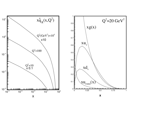
Figure 1: Parton distributions in pion and proton.

In figure (1) the shape of these partons in pion and proton is shown. It is a well known fact that there are soft partons in the hadron which cannot be evaluated in the realms of QCD. In many global fits to data this nonperturbative components are considered in rather ad hoc. basis. In our model it turns out that the results fall a few percent bellow the experimental values. We attribute this shortfall to the presence of soft gluons in proton which binds CQs to form a physical hadron. These soft gluons are parameterized.The soft gluon can fluctuate into a pair of $\bar{q}-q$. After such a pair is created a $\bar{u}$ can couple to a D-type CQ to form an intermediate $\pi^{-}=D\bar{u}$ while the $u$ quark combines with the other two U-type CQs to form a $\Delta^{++}$. Similarly, a $\bar{d}d$ can fluctuate into a $\pi^{+}n$ state. Since $\Delta^{++}$ state is more massive than $n$ state, the probability of $\bar{d}d$ fluctuation will dominate and that leads to an excess of $\bar{d}d$ pairs over $\bar{u}u$. This process is responsible for the $SU(2)$ symmetry and the violation of Gottfried Sum rule  $\!{}^{{\bf?}}$, and Ref.[1]. The result of such a calculation is depicted in Fig. (2) and it is compared with the experimental results from Fermilab E866.

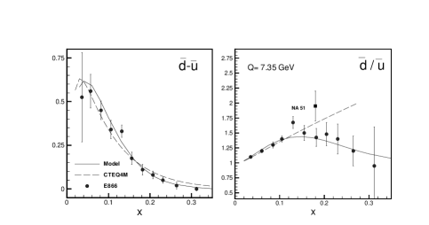
Figure 2: The ratio $\frac{\bar{d}}{\bar{u}}$ and the difference $\bar{d}-\bar{u}$ as a function of $x$. The solid line in the model calculation.

Adding this nonperturbative contribution to the constituent quark contribution will complete the evaluation of proton structure function $F_{2}^{p}$. As it can be seen in Fig. (3) our model calculation agrees rather well with HERA data in a wide range of kinematics both in $x$ and $Q^{2}$.

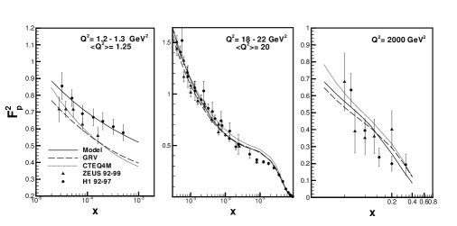
Figure 3: Proton structure function $F_{2}^{p}$ as a function of $x$ calculated using the model and compared with the data.

1 APPENDIX

In this appendix we will give the functional form of parameters of Eqs. (4, 5) in terms of the evolution parameter, $t$. This will completely determines partonic structure of CQ and their evolution. The results are valid for three and four flavors, although the flavor number is not explicitly present but they have entered in through the calculation of moments. As we explained in the text, we have taken the number of flavors to be three for $Q^{2}\leq 5GeV^{2}$ and four for higher $Q^{2}$ values.

I) Valence quark in CQ (Eq. 4):

$a=-0.1512+1.785t-1.145t^{2}+0.2168t^{3}$
$b=1.460-1.137t+0.471t^{2}-0.089t^{3}$
$c=-1.031+1.037t-0.023t^{2}+0.0075t^{3}$

II) Sea quark in CQ (Eq. 5):

$\alpha=0.070-0.213t+0.247t^{2}-0.080t^{3}$
$\beta=0.336-1.703t+1.495t^{2}-0.455t^{3}$
$\gamma=-20.526+57.495t-46.892t^{2}+12.057t^{3}$
$\eta=3.187-9.141t+10.000t^{2}-3.306t^{3}$
$\xi=-7.914+19.177t-18.023t^{2}+5.279t^{3}$

III) Gluon in CQ (Eq. 5)

$\alpha=0.826-1.643t+1.856t^{2}-0.564t^{3}$
$\beta=0.328-1.363t+0.950t^{2}-0.242t^{3}$
$\gamma=-0.482+1.528t-0.223t^{2}-0.023t^{3}$
$\eta=0.480-3.386t+4.616t^{2}-1.441t^{3}$
$\xi=-2.375+6.873t-7.458t^{2}+2.161t^{3}$

References

References

• [1] F. Arash and Ali N. Khorramian, Hep-ph/0003157.
• [2] J.Magnin and H. R. Christinsen,Phys. Rev. D 61, 054006 (2000).