SOGANG-HEP 284/01

Static properties of chiral models

with SU(3) group structure

Soon-Tae Hong^1,2 and Young-Jai Park¹

¹Department of Physics, Sogang University, Seoul 100-611, Korea

²W.K. Kellogg Radiation Laboratory, California Institute of Technology, Pasadena, CA 91125, USA

We investigate the strangeness in the framework of chiral models, such as the Skyrmion, MIT bag, chiral bag and superqualiton models, with SU(3) flavor group structure. We review the recent progresses in both the theoretical paradigm and experimental verification for strange hadron physics, and in particular the SAMPLE experiment results on the proton strange form factor. We study the color flavor locking phase in the color superconducting quark matter at high density, which might exist in the core of neutron stars, in the soliton-like superqualiton description. We explain the difficulties encountered in the application of the standard Dirac quantization to the Skyrmion and superqualiton models and treat the geometrical constraints of these soliton models properly to yield the relevant mass spectrum including the Weyl ordering corrections and the BRST symmetry structures.

PACS: 21.60.Fw, 12.39.Dc, 13.40.Gp, 14.20.-c, 11.10.Ef, 12.20.Ds
Keywords: chiral models, Skyrmions, form factors, Dirac formalism, superqualiton

1 Introduction

Nowadays there has been significant discussion concerning the possibility of sizable strange quark matrix elements in the nucleon. Especially the measurement of the spin structure function of the proton given by the European Muon Collaboration (EMC) experiments on deep inelastic muon scattering [1] has suggested a lingering question touched on by physicists that the effect of strange quarks on nucleon structure is not small. The EMC result has been interpreted as the possibility of a strange quark sea strongly polarized opposite to the proton spin. Similarly such interpretation of the strangeness has been brought to other analyzes of low energy elastic neutrino-proton scattering[2].

Quite recently, the SAMPLE Collaboration[3, 4] reported the experimental data of the proton strange form factor through parity violating electron scattering [5, 6, 7]. To be more precise, they measured the neutral weak form factors at a small momentum transfer $Q_{S}^{2}=0.1~{}{\rm(GeV/c)}^{2}$ to yield the proton strange magnetic form factor [3, 4]

$$G_{M}^{s}(Q_{S}^{2})=+0.14\pm 0.29~{}{\rm(stat)}\pm 0.31~{}{\rm(sys)}.$$

This result is contrary to the negative values of the proton strange form factor which result from most of the model calculations [8, 9, 10, 11, 12, 13, 14, 15, 16, 17, 18, 19, 20, 21, 22] except those of Hong, Park and Min [23, 24, 25] based on the SU(3) chiral bag model (CBM) [26, 27, 28, 29, 30, 31, 32, 33, 34, 35, 36, 37, 38, 39, 40, 41, 42, 43] and the recent predictions of the chiral quark soliton model [44] and the heavy baryon chiral perturbation theory [45, 46]. Recently the anapole moment effects associated with the parity violating electron scattering have been intensively studied to yield the more theoretical predictions [46, 47, 48, 49, 50]. (For details see Ref. [50].)

In fact, if the strange quark content in the nucleon is substantial then kaon condensation can be induced at a matter density lower than that of chiral phase transition [51, 52] affecting the scenarios for relativistic heavy-ion reactions [53], neutron star cooling [54, 55, 56, 57, 58, 59, 60, 61, 62, 63] and so on.

On the other hand, it is well known that baryons can be obtained from topological solutions, known as SU(2) Skyrmions, since the homotopy group $\Pi_{3}(SU(2))=Z$ admits fermions [64, 31, 65, 66, 67]. Using the collective coordinates of the isospin rotation of the Skyrmion, Witten and co-workers [64] have performed semiclassical quantization having the static properties of baryons within 30$\%$ of the corresponding experimental data.

Phenomenologically, the MIT bag model [68, 69] firstly incorporated confinement and asymptotic freedom of QCD. However, this model lacks chiral symmetry so that it cannot be directly applied to the nuclear interaction description. Moreover, in order for the bag to be stable, a bag size should be approximately 1 fm, which is simply too big to naively exploit the MIT bag model in describing nuclear systems. To overcome these difficulties, Brown and Rho proposed a ”little bag” [26, 27] where they implemented the spontaneously broken chiral symmetry and brought in Goldstine pion cloud to yield the pressure enough to squeeze the bag to a smaller size so that the bag can accommodate the nuclear physics of meson exchange interactions. Here how to squeeze the bag without violating the uncertainty principle will be discussed later in accordance with the Cheshire cat principle [70]. On the other hand, the pion cloud was introduced outside the MIT bag to yield a ”chiral bag” [71] by imposing chiral invariant boundary conditions associated with the chiral invariance and confinement.

As shown in the next chapter, based on an analogy to the monopole-isomultiplet system [72], the baryon number was firstly noticed [73] to be fractionalized into the quark and pion phase contributions, and later established [31] for the special case of the ”magic angle” of the pionic hedgehog field and then generalized for arbitrary chiral angle [74]. Here one notes that, in the ”cloud bag” model [75], the hedgehog component of the pion field was ignored so that the baryon number could be lodged entirely inside the bag.

The CBM, which is a hybrid of two different models: the MIT bag model at infinite bag radius on one hand and the SU(3) Skyrmion model at vanishing radius on the other hand, has enjoyed considerable success in predictions of the baryon static properties such as the EMC experiments and the magnetic moments of baryon octet and decuplet, as well as the strange form factors of baryons[23] to confirm the SAMPLE Collaboration experiments. After the discovery of the Cheshire cat principle [70], the CBM has been also regarded as a candidate which unifies the MIT bag and Skyrmion models and gives model independent relations insensitive to the bag radius.

On the other hand, Brown and co-workers [28] calculated the pion cloud contributions to the baryon magnetic moments by using the SU(2) CBM as an effective nonrelativistic quark model (NRQM). The Coleman-Glashow sum rules of the magnetic moments of the baryon octet were investigated in the SU(3) CBM so that the bag was proposed as an effective NRQM with meson cloud inside and outside the bag surface [37]. The possibility of unification of the NRQM and Skyrmion and MIT bag models through the chiral bag, was proposed again for the baryon decuplet [38], as well as the baryon octet [37].

In the Skyrmion model [76, 66], many properties of baryon containing light u- and d-quarks have suggested that they can be described in terms of solitons. Provided the Wess-Zumino term [77] is included in the nonlinear sigma model Lagrangian, the solitons have the correct quantum numbers to be QCD baryons [78] with many predictions of their static properties [64]. Moreover the $N_{c}$ counting suggests that the baryons with a single heavy quark ($m_{q}\gg\Lambda_{QCD}$) can be described as solitons as baryon containing only light quarks.

Meanwhile, there has been considerable progress in understanding the properties of baryons containing a single heavy quarks [79, 80]. Callan and Klebanov (CK) [79] suggested an interpretation of baryons containing heavy quarks as bound states of solitons of the pion chiral Lagrangian with mesons containing heavy quark. In their formalism, the fluctuations in the strangeness direction are treated differently from those in the isospin directions [79, 80]. Jenkins and Manohar [81] recently reconsidered the model in terms of the heavy quark symmetry to conclude that a doublet of mesons containing the heavy quark can take place in the bound state if both the soliton and meson are taken as infinitely heavy. On the other hand, in the scheme of the SU(3) cranking, Yabu and Ando [82] proposed the exact diagonalization of the symmetry breaking terms by introducing the higher irreducible representation (IR) mixing in the baryon wave function, which was later interpreted in terms of the multiquark structure [83, 84] in the baryon wave function.

On the other hand, the Dirac method [85] is a well known formalism to quantize physical systems with constraints. The string theory is known to be restricted to obey the Virasoro conditions, and thus it is quantized [86] by the Dirac method. The Dirac quantization scheme has been also applied to the nuclear phenomenology [87, 88]. In this method, the Poisson brackets in a second-class constraint system are converted into Dirac brackets to attain self-consistency. The Dirac brackets, however, are generically field-dependent, nonlocal and contain problems related to ordering of field operators. These features are unfavorable for finding canonically conjugate pairs. However, if a first-class constraint system can be constructed, one can avoid introducing the Dirac brackets and can instead use Poisson brackets to arrive at the corresponding quantum commutators.

To overcome the above problems, Batalin, Fradkin, and Tyutin (BFT) [89] developed a method which converts the second-class constraints into first-class ones by introducing auxiliary fields. Recently, this BFT formalism has been applied to several models of current interest [90, 91, 92, 93], especially to the Skyrmion to obtain the modified mass spectrum of the baryons by including the Weyl ordering correction [94, 95, 96, 97].

Furthermore, due to asymptotic freedom [98, 99], the stable state of matter at high density will be quark matter [100], which has been shown to exhibit color superconductivity at low temperature [101, 102]. The color superconducting quark matter [103, 104, 105, 106, 107, 108, 109, 110, 111, 112, 113, 114, 115, 116, 117, 118, 119, 120, 121, 122, 123, 124, 125, 126, 127, 128, 129, 130, 131, 132, 133, 134, 135, 136] might exist in the core of neutron stars, since the Cooper-pair gap and the critical temperature turn out to be quite large, of the order of $10\sim 100~{}{\rm MeV}$, compared to the core temperature of the neutron star, which is estimated to be up to $\sim 0.7$ MeV [137]. On the other hand, it is found that, when the density is large enough for strange quark to participate in Cooper-pairing, not only color symmetry but also chiral symmetry are spontaneously broken due to so-called color-flavor locking (CFL) [115]: At low temperature, Cooper pairs of quarks form to lock the color and flavor indices as

$$\left<{\psi_{L}}^{a}_{i\alpha}(\vec{p}){\psi_{L}}^{b}_{j\beta}(-\vec{p})\right>=-\left<{\psi_{R}}^{a}_{i\alpha}(\vec{p}){\psi_{R}}^{b}_{j\beta}(-\vec{p})\right>=\epsilon_{\alpha\beta}\epsilon^{abI}\epsilon_{ijI}\Delta(p_{F}),$$ (1.1)

where $a,b=1,2,3$ and $i,j=1,2,3$ are color and flavor indices, respectively, and we ignore the small color sextet component in the condensate. In this CFL phase, the particle spectrum can be precisely mapped into that of the hadronic phase at low density. Observing this map, Schäfer and Wilczek [109, 108] have further conjectured that two phases are in fact continuously connected to each other. The CFL phase at high density is complementary to the hadronic phase at low density. This conjecture was subsequently supported by showing that quarks in the CFL phase are realized as Skyrmions, called superqualitons, just like baryons are realized as Skyrmions in the hadronic phase [113, 134].

2 Outline of the chiral models

2.1 Chiral symmetry and currents

For a fundamental theory of hadron physics, we will consider in this work the chiral models such as Skyrmion, MIT bag and chiral bag models. Especially, the CBM can be described as a topological extended object with hybrid phase structure: the quark fields surrounded by the meson cloud outside the bag. In the CBM, a surface coupling with the meson fields is introduced to restore the chiral invariance [71] which was broken in the MIT bag [68, 69]. To discuss the symmetries of the CBM and to derive the vector and axial currents, which are crucial ingredients for the physical operators for the magnetic moments and EMC experiments, we introduce the realistic chiral bag Lagrangian

$${\cal L}={\cal L}_{CS}+{\cal L}_{CSB}+{\cal L}_{FSB}$$ (2.1)

with the chiral symmetric (CS) part, chiral symmetry breaking (CSB) mass terms and SU(3) flavor symmetry breaking (FSB) pieces due to the corrections $m_{\pi}\neq m_{K}$ and $f_{\pi}\neq f_{K}$

$${\cal L}_{CS} = \bar{\psi}i\gamma^{\mu}\partial_{\mu}\psi-\frac{1}{2}\bar{\psi}U_{5}\psi\Delta_{B}$$

$$+\left(-\frac{1}{4}f_{\pi}^{2}{\rm tr}(l_{\mu}l^{\mu})+\frac{1}{32e^{2}}{\rm tr}[l_{\mu},l_{\nu}]^{2}+{\cal L}_{WZW}\right)\bar{\Theta}_{B}$$

$${\cal L}_{CSB} = -\bar{\psi}M\psi\Theta_{B}+\frac{1}{4}f_{\pi}^{2}m_{\pi}^{2}{\rm tr}(U+U^{\dagger}-2)\bar{\Theta}_{B}$$

$${\cal L}_{FSB} = \frac{1}{6}(f_{\pi}^{2}m_{K}^{2}-f_{\pi}^{2}m_{\pi}^{2}){\rm tr}((1-\sqrt{3}\lambda_{8})(U+U^{\dagger}-2))\bar{\Theta}_{B}$$ (2.2)

$$-\frac{1}{12}f_{\pi}^{2}(\chi^{2}-1){\rm tr}((1-\sqrt{3}\lambda_{8})(Ul_{\mu}l^{\mu}+l_{\mu}l^{\mu}U^{\dagger}))\bar{\Theta}_{B}.$$

Here the quark field $\psi$ has SU(3) flavor degrees of freedom and the chiral field $U=e^{i\lambda_{a}\pi_{a}/f_{\pi}}\in$ SU(3) is described by the pseudoscalar meson fields $\pi_{a}$ $(a=1,...,8)$ and Gell-Mann matrices $\lambda_{a}$ with $\lambda_{a}\lambda_{b}=\frac{2}{3}\delta_{ab}+(if_{abc}+d_{abc})\lambda_{c}$, and $l_{\mu}=U^{\dagger}\partial_{\mu}U$. In the numerical calculation in the CBM we will use the parameter fixing $e=4.75$, $f_{\pi}=93$ MeV and $f_{K}=114$ MeV.

The interaction term crucial for the chiral symmetry restoration is given by

$$U_{5}=\frac{1+\gamma_{5}}{2}U\frac{1+\gamma_{5}}{2}+\frac{1-\gamma_{5}}{2}U^{\dagger}\frac{1-\gamma_{5}}{2},$$ (2.3)

and $\Delta_{B}=-n^{\mu}\partial_{\mu}\Theta_{B}$ where $\Theta_{B}$ is the bag theta function with vanishing value (normalized to be unity) only inside the bag and $n^{\mu}$ is the outward normal unit four vector and the Skyrmion term is included to stabilize soliton solution of the meson phase Lagrangian in ${\cal L}_{CS}$. The WZW term, which will be discussed in terms of the topology in the next section, is described by the action

$$\Gamma_{WZW}=-\frac{iN_{c}}{240\pi^{2}}\int_{\bar{{\sf M}}}{\rm d}^{5}r\epsilon^{\mu\nu\alpha\beta\gamma}{\rm tr}(l_{\mu}l_{\nu}l_{\alpha}l_{\beta}l_{\gamma}),$$ (2.4)

where $N_{c}$ is the number of colors and the integral is done on the five-dimensional manifold $\bar{{\sf M}}=\bar{V}\times S^{1}\times I$ with the three-space volume $\bar{V}$ outside the bag, the compactified time $S^{1}$ and the unit interval $I$ needed for a local form of WZW term. The chiral symmetry is explicitly broken by the quark mass term with $M={\rm diag}~{}(m_{u},m_{d},m_{s})$ and pion mass term, which is chosen such that it will vanish for $U=1$.

Now we want to construct Noether currents under the SU(3)${}_{L}\times$SU(3)_R local group transformation. Under infinitesimal isospin transformation in the SU(3) flavor channel

$$\psi\rightarrow\psi^{\prime} = (1-i\epsilon_{a}\hat{Q}_{a})\psi,$$

$$U\rightarrow U^{\prime} = (1-i\epsilon_{a}\hat{Q}_{a})U(1+i\epsilon_{a}\hat{Q}_{a}),$$ (2.5)

where $\epsilon_{a}(x)$ the local angle parameters of the group transformation and $\hat{Q}_{a}=\lambda_{a}/2$ are the SU(3) flavor charge operators given by the generators of the symmetry, the Noether theorem yields the flavor octet vector currents (FOVC) from the derivative terms in ${\cal L}_{CS}$ and ${\cal L}_{FSB}$

$$J_{V}^{\mu a} = \bar{\psi}\gamma^{\mu}\hat{Q}_{a}\psi\Theta_{B}+\left(-\frac{i}{2}f_{\pi}^{2}{\rm tr}(\hat{Q}_{a}l^{\mu})+\frac{i}{8e^{2}}{\rm tr}[\hat{Q}_{a},l^{\nu}][l^{\mu},l^{\nu}]+U\leftrightarrow U^{\dagger}\right)\bar{\Theta}_{B}$$ (2.6)

$$-\frac{i}{12}(f_{K}^{2}-f_{\pi}^{2}){\rm tr}((1-\sqrt{3}\lambda_{8})(U\{\hat{Q}_{a},l^{\mu}\}+\{\hat{Q}_{a},l^{\mu}\}U^{\dagger})+U\leftrightarrow U^{\dagger})\bar{\Theta}_{B}$$

$$+\frac{N_{c}}{48\pi^{2}}\epsilon^{\mu\nu\alpha\beta}{\rm tr}(\hat{Q}_{a}l_{\nu}l_{\alpha}l_{\beta}-U\leftrightarrow U^{\dagger})\bar{\Theta}_{B}$$

with $\epsilon^{0123}=1$. Of course the $J_{V}^{\mu a}$ are conserved as expected in the chiral limit, but the mass terms in ${\cal L}_{CSB}$ and ${\cal L}_{FSB}$ give rise to the nontrivial four-divergence

$$\partial_{\mu}J_{V}^{\mu a} = -\frac{i}{6}(f_{K}^{2}m_{K}^{2}-f_{\pi}^{2}m_{\pi}^{2}){\rm tr}((1-\sqrt{3}\lambda_{8})[\hat{Q}_{a},U+U^{\dagger}])\bar{\Theta}_{B}$$ (2.7)

$$+\frac{i}{12}(f_{K}^{2}-f_{\pi}^{2}){\rm tr}((1-\sqrt{3}\lambda_{8})[\hat{Q}_{a},Ul_{\mu}l^{\mu}+l_{\mu}l^{\mu}U^{\dagger}])\bar{\Theta}_{B}$$

$$-i\bar{\psi}[\hat{Q}_{a},M]\psi\Theta_{B}.$$

In addition one can see that the electromagnetic (EM) currents $J_{EM}^{\mu}$ can be easily constructed by replacing the SU(3) flavor charge operators $\hat{Q}_{a}$ with the EM charge operator $\hat{Q}_{EM}=\hat{Q}_{3}+\frac{1}{\sqrt{3}}\hat{Q}_{8}$ in the FOVC (2.6) and that the four divergence (2.7) vanishes to yield the conserved EM currents.

Similarly under infinitesimal chiral transformation in the SU(3) flavor channel

$$\psi\rightarrow\psi^{\prime} = (1-i\epsilon_{a}\gamma_{5}\hat{Q}_{a})\psi,$$

$$U\rightarrow U^{\prime} = (1+i\epsilon_{a}\hat{Q}_{a})U(1+i\epsilon_{a}\hat{Q}_{a}),$$ (2.8)

one obtains the flavor octet axial currents (FOAC)

$$J_{A}^{\mu a} = \bar{\psi}\gamma^{\mu}\gamma_{5}\hat{Q}_{a}\psi\Theta_{B}+\left(-\frac{i}{2}f_{\pi}^{2}{\rm tr}(\hat{Q}_{a}l^{\mu})+\frac{i}{8e^{2}}{\rm tr}[\hat{Q}_{a},l^{\nu}][l^{\mu},l^{\nu}]-U\leftrightarrow U^{\dagger}\right)\bar{\Theta}_{B}$$ (2.9)

$$-\frac{i}{12}(f_{K}^{2}-f_{\pi}^{2}){\rm tr}((1-\sqrt{3}\lambda_{8})(U\{\hat{Q}_{a},l^{\mu}\}+\{\hat{Q}_{a},l^{\mu}\}U^{\dagger})-U\leftrightarrow U^{\dagger})\bar{\Theta}_{B}$$

$$+\frac{N_{c}}{48\pi^{2}}\epsilon^{\mu\nu\alpha\beta}{\rm tr}(\hat{Q}_{a}l_{\nu}l_{\alpha}l_{\beta}+U\leftrightarrow U^{\dagger})\bar{\Theta}_{B}.$$

Here one notes that the FOAC are conserved only in the chiral limit, but one has the nontrivial four-divergence from the mass terms of ${\cal L}_{CSB}$ and ${\cal L}_{FSB}$

$$\partial_{\mu}J_{A}^{\mu a} = \frac{i}{6}(f_{K}^{2}m_{K}^{2}-f_{\pi}^{2}m_{\pi}^{2}){\rm tr}((1-\sqrt{3}\lambda_{8})[\hat{Q}_{a},U-U^{\dagger}])\bar{\Theta}_{B}$$ (2.10)

$$-\frac{i}{12}(f_{K}^{2}-f_{\pi}^{2}){\rm tr}((1-\sqrt{3}\lambda_{8})\{\hat{Q}_{a},Ul_{\mu}l^{\mu}-l_{\mu}l^{\mu}U^{\dagger}\})\bar{\Theta}_{B}$$

$$+i\bar{\psi}\gamma_{5}\{\hat{Q}_{a},M\}\psi\Theta_{B}.$$

In the meson phase currents of (2.6) and (2.9), one should note that the terms with $U\leftrightarrow U^{\dagger}$ in the FOAC have the opposite sign of those in the FOVC. Moreover the mesonic currents from the WZW term and the nontopological terms have also the sign difference in front of the term with $U\leftrightarrow U^{\dagger}$.

On the other hand, one can define the sixteen vector and axial vector charges [138, 139, 140] of SU(3)${}_{L}\times$SU(3)_R

$$\hat{Q}_{a} = \int{\rm d}^{3}xJ_{V}^{0a}$$

$$\hat{Q}_{a}^{5} = \int{\rm d}^{3}xJ_{A}^{0a}$$ (2.11)

where $J_{V}^{\mu a}$ and $J_{A}^{\mu a}$ are the octets of the FOVC and FOAC in (2.6) and (2.9) respectively. In the quantized theory discussed later these generators are the charge operators and satisfy their equal time commutator relations of the Lie algebra of SU(3)${}_{L}\times$SU(3)_R

$$\left[\hat{Q}_{a},\hat{Q}_{b}\right] = if_{abc}\hat{Q}_{c}$$

$$\left[\hat{Q}_{a},\hat{Q}_{b}^{5}\right] = if_{abc}\hat{Q}_{c}^{5}$$

$$\left[\hat{Q}_{a}^{5},\hat{Q}_{b}^{5}\right] = if_{abc}\hat{Q}_{c}$$ (2.12)

and the chiral charges $\hat{Q}_{a}^{R}$ and $\hat{Q}_{a}^{L}$ defined as

$$\hat{Q}_{a}^{R,L}=\frac{1}{2}(\hat{Q}_{a}\pm\hat{Q}_{a}^{5})$$ (2.13)

form a disjoint Lie algebra of SU(3)s

$$\left[\hat{Q}_{a}^{R},\hat{Q}_{b}^{R}\right] = if_{abc}\hat{Q}_{c}^{R}$$

$$\left[\hat{Q}_{a}^{L},\hat{Q}_{b}^{L}\right] = if_{abc}\hat{Q}_{c}^{L}$$

$$\left[\hat{Q}_{a}^{R},\hat{Q}_{b}^{L}\right] = 0$$ (2.14)

from which the Adler-Weisberger sum rules [141, 142] can be obtained in terms of off-mass shell pion-nucleon cross sections.

2.2 WZW action and baryon number

More than thirty years ago Skyrme [76] proposed a picture of the nucleon as a soliton in the otherwise uniform vacuum configuration of the nonlinear sigma model. Quantizing the topologically twisted soliton, he suggested that the topological charge or winding number could be identified with baryon number $B$. His conjecture for the definition of $B$ has been revived [78, 143] in terms of quantum chromodynamics (QCD). In particular Witten [78] has established a unique relation between the topological charge and baryon number with the number of colors $N_{c}$ playing a crucial role.

In the large-$N_{c}$ limit of QCD [144], meson interactions are described by the tree approximation to an effective local field theory of mesons, and baryons behave as if they were solitons [145] so that the identification of the Skyrmion with a baryon can be consistent with QCD.

In this section we will briefly review and summarize the fermionization of the Skyrmion with the WZW action [78] to obtain the baryon number in the CBM.

Now we consider the pure Skyrmion on a space-time manifold compactified to be $S^{4}=S^{3}\times S^{1}$ where $S^{3}$ and $S^{1}$ are compactified Euclidean three-space and time respectively. The chiral field $U$ is then a mapping of $S^{4}$ into the SU(3) group manifold to yield the homotopy group $\pi_{4}($SU(3)$)=0$ so that the four-sphere in SU(3) defined by $U(x)$ is the boundary of a five dimensional manifold ${\sf M}=S^{3}\times S^{1}\times I$ with two dimensional disc $D=S^{1}\times I$ where $I$ is the unit interval. Here one notes that ${\sf M}$ is not unique so that the compactified space-time $S^{4}$ is also the boundary of another five-disc ${\sf M}^{\prime}$ with opposite orientation.

On the SU(3) manifold there is a unique fifth rank antisymmetric tensor $\omega_{\mu\nu\alpha\beta\gamma}$ invariant under SU(3)${}_{L}\times$SU(3)_R, which enables us to define an action

$$\Gamma_{{\sf M},{\sf M}^{\prime}}=\pm\int_{{\sf M},{\sf M}^{\prime}}{\rm d}^{5}x\epsilon^{\mu\nu\alpha\beta\gamma}\omega_{\mu\nu\alpha\beta\gamma},$$ (2.15)

where the signs $\pm$ are due to the orientations of the five-discs ${\sf M}$ and ${\sf M}^{\prime}$ respectively. As in Dirac quantization for the monopole [146, 147], one should demand the uniqueness condition in a Feynman path integral $e^{i\Gamma}{\sf M}=e^{i\Gamma}{\sf M}^{\prime}$ to yield $\Gamma_{\sf M}-\Gamma_{{\sf M}^{\prime}}=\int_{{\sf M}+{\sf M}^{\prime}}\omega=2\pi\times$integer for any five-sphere constructed from ${\sf M}+{\sf M}^{\prime}$ in the SU(3) group manifold. Here one notes that every five-sphere in SU(3) is topologically a multiple of a basic five-sphere $S^{5}$ due to $\pi_{5}$(SU(3))=$Z$. Normalizing $\omega$ on the basic five-sphere $S^{5}$ such that $\int_{S^{5}}\omega=2\pi$ one can use in the quantum field theory the action of the form $n\Gamma$ where $n$ is an arbitrary integer. On the other hand one can obtain the fifth rank antisymmetric tensor $\omega_{\mu\nu\alpha\beta\gamma}$ on the five-disc ${\sf M}$ [78]

$$\omega_{\mu\nu\alpha\beta\gamma}=-\frac{i}{240\pi^{2}}{\rm tr}(l_{\mu}l_{\nu}l_{\alpha}l_{\beta}l_{\gamma}),$$ (2.16)

which leads us to the condition that the $n\Gamma_{\sf M}$ is nothing but the WZW term in the pure Skyrmion model if $n=N_{c}$. Here one notes in the weak field approximation that the right hand side of (2.16) can be reduced into a total divergence so that by Stokes’s theorem $\int_{\sf M}\omega$ can be rewritten as an integral over the boundary of ${\sf M}$, namely compactified space-time $S^{5}$. In the CBM the five-disc ${\sf M}=S^{3}\times S^{1}\times I$ is modified into $\bar{{\sf M}}=\bar{V}\times S^{1}\times I$ where $\bar{V}=S^{3}-V$ with $V$ being the three-space volume inside the bag. On the modified five-manifold one can construct the WZW term (2.4) in the CBM.

Also it is shown [78] that the above action $\Gamma_{\sf M}$ is a homotopy invariant under SU(2) mappings with the homotopy group $\pi_{4}$(SU(2))=$Z_{2}$ and for a $2\pi$ adiabatic rotation of a soliton the action gains the value $\Gamma_{\sf M}=\pi$ corresponding to the nontrivial homotopy class in $\pi_{4}$(SU(2)) so that one can obtain an extra phase $e^{in\pi}=(-1)^{n}$ in the amplitude, with respect to a soliton at rest with $\Gamma_{\sf M}=0$ belonging to the trivial homotopy class. Here the factor $(-1)^{n}$ indicates that the soliton is a fermion (boson) for odd (even) $n$. On the other hand, one remembers that a baryon constructed with $n$ quarks is a fermion (boson) if $n$ is odd (even). With the WZW term with three flavor $N_{c}=3$, one then concludes that the Skyrmion can be fermionized. Here one notes that the nontrivial homotopy class in $\pi_{4}$(SU(2)) can be depicted [78] by the creation and annihilation mechanism of a Skyrmion-anti Skyrmion pair in the vacuum through the channel of $2\pi$ rotation of the Skyrmion and it corresponds to quantization of the Skyrmion as a fermion. Such a mechanism has also been used [148] in the (2+1) dimensional nonlinear sigma model to discuss the Hopf topological invariant and linking number [149].

In fact, since the (2+1) dimensional O(3) nonlinear sigma model (NLSM) was first discussed by Belavin and Polyakov [150], there have been lots of attempts to improve this soliton model associated with the homotopy group $\pi_{2}(S^{2})=Z$. In particular, the configuration space in the O(3) NLSM is infinitely connected to yield the fractional spin statistics, which was first shown by Wilczek and Zee [151, 149] via the additional Hopf term. Moreover the O(3) NLSM with the Hopf term was canonically quantized [152] and the $CP^{1}$ model with the Hopf term [153, 154, 155, 156, 157], which can be related with the O(3) NLSM via the Hopf map projection from $S^{3}$ to $S^{2}$, was also canonically quantized later [154]. In fact, the $CP^{1}$ model has better features than the O(3) NLSM, in the sense that the action of the $CP^{1}$ model with the Hopf invariant has a desirable manifest locality, since the Hopf term has a local integral representation in terms of the physical fields of the $CP^{1}$ model [149]. Furthermore, this manifest locality in time is crucial for a consistent canonical quantization [158]. Recently, the geometrical constraints in the O(3) NLSM and $CP^{1}$ model are systematically analyzed to yield the first class Hamiltonian and the corresponding BRST invariant effective Lagrangian [159, 160, 158]. Meanwhile, the $CP^{N}$ model was studied [161] on the noncommutative geometry [162], which was quite recently analyzed in the framework of the improved Dirac quantization scheme [163].

Now using the Noether theorem as in the previous section one can obtain the conserved flavor singlet vector currents (FSVC) $J_{V}^{\mu}$ which can be practically derived by simple replacement of $\hat{Q}_{a}$ with 1 in the FOVC (2.6). If one defines the baryon number of a quark to be $1/N_{c}$ so that a baryon constructed from $N_{c}$ quarks has baryon number one, then the baryon number current $B^{\mu}$ can be shown to be $(1/N_{c})J_{V}^{\mu}$, namely

$$B^{\mu}=\frac{1}{N_{c}}\bar{\psi}\gamma^{\mu}\psi\Theta_{B}+\frac{1}{24\pi^{2}}\epsilon^{\mu\nu\alpha\beta}{\rm tr}(l_{\nu}l_{\alpha}l_{\beta})\bar{\Theta}_{B},$$ (2.17)

and the baryon number of the chiral bag is given by

$$B=\int{\rm d}^{3}xB^{0}=\int_{B}{\rm d}^{3}x\frac{1}{N_{c}}\psi^{\dagger}\psi+\int_{\bar{V}}{\rm d}^{3}x\frac{1}{24\pi^{2}}\epsilon_{ijk}{\rm tr}(l_{i}l_{j}l_{k}),$$ (2.18)

which will be discussed in terms of the hedgehog solution ansatz in the next section.

2.3 Hedgehog solution

Since the Euler equation for the meson fields in the nonlinear sigma model was analytically investigated [71] to obtain a specific classical solution for the meson fields whose isospin index points radially $\pi_{i}(\vec{r})/f_{\pi}=\hat{r}^{i}\theta(r)$, the so-called hedgehog solution, this spherically symmetric classical solution has been commonly used as a prototype ansatz in the literature of the Skyrmion related hadron physics.

In this section we will consider the classical configuration in the meson and quark phases to review and summarize briefly the baryon number fractionization [31, 74] in the CBM.

Assuming maximal symmetry in the meson phase of the chiral bag, we describe the hedgehog solution $U_{0}$ embedded in the SU(2) isospin subgroup of SU(3)

$$U_{0}=\left(\begin{array}[]{cc}e^{i\vec{\tau}\cdot\hat{r}\theta(r)}&0\\ 0&1\\ \end{array}\right)$$ (2.19)

where $\tau_{i}$ $(i=1,2,3)$ are the Pauli matrices, $\hat{x}=\vec{x}/r$ and $\theta(r)$ is the chiral angle determined by minimizing the static mass $M$ of the chiral bag and constrained by the boundary condition at the bag surface.

In the CBM Lagrangian (2.1), due to the symmetry breaking mass terms, the static mass has an additional pion mass term [65, 66, 164] as below

$$M = \frac{2\pi f_{\pi}}{e}\int_{ef_{\pi}R}^{\infty}{\rm d}z~{}z^{2}\left(\left(\frac{d\theta}{dz}\right)^{2}+\left(2+2\left(\frac{d\theta}{dz}\right)^{2}+\frac{\sin^{2}\theta}{z^{2}}\right)\frac{\sin^{2}\theta}{z^{2}}\right.$$ (2.20)

$$\left.+2\mu_{\pi}^{2}(1-\cos\theta)\right)$$

with the dimensionless quantities $z=ef_{\pi}r$ and $\mu_{\pi}=m_{\pi}/ef_{\pi}$. Minimizing the above static mass $M$, one obtain the equation of motion for the chiral angle $\theta$ outside the bag

$$(z^{2}+2\sin^{2}\theta)\frac{d^{2}\theta}{dz^{2}}+2z\frac{d\theta}{dz}+\left(\left(\frac{d\theta}{dz}\right)^{2}-1-\frac{\sin^{2}\theta}{z^{2}}\right)\sin 2\theta$$

$$-\mu_{\pi}^{2}z^{2}\sin\theta=0$$ (2.21)

which yields the static Skyrmion chiral angle defining a stationary point of the chiral bag action.

Together with the boundary term $-\frac{1}{2}\bar{\psi}U_{5}\psi\Delta_{B}$, the static mass $M$ also yields the boundary condition for the chiral angle at $z=ef_{\pi}R$

$$\left(1+\frac{2\sin^{2}\theta}{z^{2}}\right)\frac{d\theta}{dz}=\frac{1}{2ef_{\pi}^{3}}\bar{\psi}i\gamma_{5}\vec{\tau}\cdot\hat{r}e^{i\gamma_{5}\vec{\tau}\cdot\hat{r}\theta}\psi$$ (2.22)

which allows the flow of currents in the two phase via the bag boundary. Here one notes that the baryon number (2.18) obtained from the topological WZW term and quark fields remains constant [31, 74] regardless of the bag radius through the continuity of the current at the bag boundary, even though one has the additional pion mass term in the static mass $M$.

On the other hand, in the chiral symmetric limit, the conventional variation scheme with respect to the quark fields yields the Dirac equation inside the bag and the boundary condition on the bag surface

$$i\gamma^{\mu}\partial_{\mu}\psi = 0,~{}~{}~{}~{}r<R,$$ (2.23)

$$i\gamma^{\mu}n_{\mu}\psi = U_{5}\psi,~{}~{}r=R$$ (2.24)

where the missing quark masses will be discussed later after the collective coordinate quantization is performed.

Due to the coupling of spin and isospin in the boundary condition (2.24), the u and d quarks can be coalesced [165] into hedgehog (h) quark states, eigenstates of grand spin $\vec{K}=\vec{I}+\vec{J}$, not of the isospin $\vec{I}$ and the spin $\vec{J}=\vec{L}+\vec{S}$ separately, while the s quark is decoupled from the hedgehog quark states. The h quark state is then specified by a set of quantum numbers $(K,m_{K},P,m)$ where $K(K+1)$ and $m_{K}$ are the eigenvalues of the squared operator $\vec{K}^{2}$ and $K_{3}$ the third component of $\vec{K}$, and $P$ and $m$ are the parity and radial excitation quantum numbers, respectively. Similarly the s quark states are labeled by another set $(j,m_{j},P,n)$ with $j(j+1)$, $m_{j}$ and $n$, the eigenvalues of $\vec{J}^{2}$, $J_{3}$ and radial quantum number.

Now the quark field $\psi$ can be expanded in terms of the wave functions of the hedgehog and strange quark states

$$\psi(\vec{r},t) = \sum_{n}\psi_{n}^{h}(\vec{r})e^{-i\varepsilon_{n}t}a_{n}+\psi_{n}^{h*}(\vec{r})e^{i\varepsilon_{n}t}b_{n}^{\dagger}$$ (2.25)

$$+\psi_{n}^{s}(\vec{r})e^{-i\omega_{n}t}c_{n}+\psi_{n}^{s*}(\vec{r})e^{i\omega_{n}t}d_{n}^{\dagger}$$

where the hedgehog quark states are expressed by the spatial wave functions $\psi_{n}^{h}(\vec{r})$ with grand spin quantum numbers, whose explicit forms will be given in the Appendix B, and the annihilation operator $a_{n}$ ($b_{n}^{\dagger}$) for the positive (negative) energy fulfills the usual anticommutator rules and also defines the vacuum $a_{n}|0>=b_{n}|0>=0$, and the strange quark states are analogously described. Here we do not bother to include the color index explicitly since every particle is a color singlet. The energy spectrum of the hedgehog quark states [165] is subordinate to $\theta(R)$, the chiral angle at bag surface, while the strange quark states remain intact regardless of the chiral angle.

Finally in the framework of the previous literatures [31, 74] we reconsider the baryon number (2.18) in the hedgehog ansatz to see that the total baryon number is still an integer in the CBM. Using the hedgehog solution (2.19) in the meson piece in (2.18) one can obtain the fractional baryon number in terms of the chiral angle at the bag surface $\theta=\theta(R)\in[-\pi,0]$ [74]

$$B_{m}=-\frac{1}{2\pi}\chi_{E}(\theta-\sin\theta\cos\theta)$$ (2.26)

where $\chi_{E}$ is the Euler characteristic, which has an inter two in the spherical bag surface.

In general the Euler characteristic of a compact surface is the topological invariant defined by the integer $v-e+f$ [166] with $v$, $e$ and $f$ the numbers of vertices, edges and faces in a decomposition of the surface so that one can easily see $\chi_{E}$(sphere) = 2 and $\chi_{E}$(torus) = 0, for instance. Also it is interesting to see that adding a handle ${\sf H}$, or a torus with the interior of one face removed, to a compact surface ${\sf S}$ reduces its Euler characteristic by two, since to obtain the coalesced surface ${\sf S^{\prime}}$ one needs the surgery of removing the interior of a face of ${\sf S}$ so that ${\sf S^{\prime}}$ has two faces less than ${\sf S}$ and ${\sf H}$ combined. For a coalesced surface with $h$ handles, one has the generalized identity $\chi_{E}({\sf S^{\prime}})=\chi_{E}({\sf S})-2h$ [166].

On the other hand, it has been noted [31] in the CBM that the quark phase spectrum is asymmetric about zero energy to yield the nonvanishing vacuum contribution to the baryon number

$$B_{0}=-\frac{1}{2}\lim_{s\rightarrow 0}\sum_{n}{\rm sgn}(E_{n})e^{-s|E_{n}|}$$ (2.27)

where the sum runs over all positive and negative energy eigenstates and the symmetrized operator $\frac{1}{2}[\psi^{\dagger},\psi]$ is used in the quark part of (2.18). Here one notes that the regularized factor is closely related [74] to the eta invariant of Atiyah et al. [167],

$$\eta(s)=\frac{1}{2}\lim_{s\rightarrow 0}\sum_{n}{\rm sgn}(E_{n})|E_{n}|^{-s}$$ (2.28)

which has been also discussed in connection with the phase factor of the path integral in quantum field theory associated with the Jones polynomial and knot theory [168], and recently has been exploited in investigation of the semiclassical partition functions and the Jacobi fields in the framework of the Morse theory of differential geometry [169].

Except at the magic angle $\theta=-\pi/2$, where the baryon number is shared equally with both quark and meson phases and $B_{0}$ jumps by unity due to the Dirac sea [31], the chiral angle dependence of the quark vacuum baryon number $dB_{0}/d\theta=\frac{1}{2}\lim_{s\rightarrow 0}\sum_{n}s(dE_{n}/d\theta)e^{-s|E_{n}|}$ is given in terms of the integration of the Gaussian curvature $\kappa$ on the bag surface ${\sf S}$ [74]

$$\frac{dB_{0}}{d\theta}=\frac{1}{2\pi^{2}}\sin^{2}\theta\int_{\sf S}{\rm d}^{2}x\kappa$$ (2.29)

where a multiple-reflection expansion of the Euclidean Green’s function, as well as the Dirac equation (2.23) and the boundary condition (2.24), has been used [74].

Using the Gauss-Bonnet theorem [170] one can rewrite (2.29) in terms of the Euler characteristic $dB_{0}/d\theta=(\chi/\pi)\sin^{2}\theta$ to yield the total quark phase baryon number

$$B_{q}=1+\frac{1}{2\pi}\chi_{E}(\theta-\sin\theta\cos\theta)$$ (2.30)

where, in addition to the $\theta$-dependent vacuum contribution $B_{0}$, one has the unity factor contributed by the $N_{c}$ degenerate valence quarks to fill the $K^{P}=0^{+}$ h-quark and $j^{P}=\frac{1}{2}^{+}$ s-quark eigenstates. In the $K^{P}=0^{+}$ level we can define the static hedgehog ground state $|H>_{0}$: $a_{v}^{\dagger}|0>$ ($a_{v}^{\dagger}$ being the valence quark creation operator with the quantum number $K^{P}=0^{+}$) for $-\pi/2\leq\theta\leq 0$ and $|0>$ in $-\pi\leq\theta<-\pi/2$, since the quarks in the positive energy level are the valence quarks while those in the negative energy level can be considered to sink into the vacuum.

Here one notes that in the MIT bag limit at $\theta=0$, where there are no vacuum and meson contributions, only the $N_{c}$ degenerate valence quarks yield the baryon number. Also for $-\pi/2\leq\theta<0$ the valence quarks and $\theta$-dependent vacuum contribute to $B_{q}$ while for $-\pi\leq\theta<-\pi/2$ only the quark vacuum does in the static hedgehog ground state.

2.4 Collective coordinate quantization

Until now we have considered the baryon quantum number in the classical static hedgehog solution in the meson phase of the CBM. As in the Skyrmion model [64], the other quantum numbers such as spin, isospin and hypercharge can be obtained in the CBM by quantizing the zero modes associated with the slow collective rotation

$$U_{0}\rightarrow AU_{0}A^{\dagger},~{}~{}~{}~{}\psi\rightarrow A\psi$$ (2.31)

on the SU(3)_F group manifold where $A(t)\in$ SU(3)_F is the time dependent collective variable restrained by the WZW constraint.

In the $\lambda$ dimensional IR, the baryon is then described by a wave function of the form

$$|B\rangle^{\lambda}=\Phi_{B}^{\lambda}(A)\otimes|{\rm intrinsic}\rangle$$ (2.32)

where $\Phi_{B}^{\lambda}(A)$ is the baryon dependent collective coordinate wave function

$$\Phi_{B}^{\lambda}(A)=\sqrt{{\rm dim}(\lambda)}D_{ab}^{\lambda}(A)$$ (2.33)

with the quantum numbers $a=(Y,I,I_{3})$ ($Y$; hypercharge, $I$; isospin) and $b=(Y_{R};J,J_{3})$ ($Y_{R}$; right hypercharge, $J$; spin) in the Wigner $D$- matrix. In the 8-dimensional adjoint representation the matrix is given by $D_{ab}^{8}(A)=\frac{1}{2}{\rm tr}(A^{\dagger}\lambda_{a}A\lambda_{b})$. On the other hand, the intrinsic state degenerate to all the baryons is described by the classical meson configuration approximated by a rotated hedgehog solution $AU_{0}A^{\dagger}$ and a rotated hedgehog ground state discussed later.

With the introduction of the collective rotation, the Dirac equation (2.23) is modified and the boundary condition (2.24) is rewritten in the hedgehog ansatz as below [33]

$$\left(i\gamma^{\mu}\partial_{\mu}+\frac{1}{2}\dot{q}_{a}\gamma^{0}\lambda_{a}\right)\psi = 0,~{}~{}~{}~{}r<R$$ (2.34)

$$\left(i\hat{r}\cdot\vec{\gamma}+e^{i\gamma_{5}\lambda_{i}\hat{r}_{i}\theta}\right)\psi = 0~{}~{}~{}~{}r=R$$ (2.35)

where we have used the collective coordinates $q_{a}$ defined by $A^{\dagger}\dot{A}=-\frac{i}{2}\lambda_{a}\dot{q}_{a}$. The collective rotation of the chiral bag induces [33] the particle-hole excitations which will be treated perturbatively in this work to yield the correction to the wave functions $\psi_{n}^{h}(\vec{r})$ and $\psi_{n}^{s}(\vec{r})$ in (2.25)

$$\psi_{n}^{h} = \psi_{n}^{0h}(\vec{r})+\frac{1}{2}\dot{q}_{i}\sum_{m\neq n}\frac{{}_{h}\langle m|\lambda_{i}|n\rangle_{h}}{\varepsilon_{m}-\varepsilon_{n}}\psi_{m}^{0h}(\vec{r})$$

$$+\frac{1}{2}\dot{q}_{p}\sum_{m}\frac{{}_{s}\langle m|\lambda_{p}|n\rangle_{h}}{\omega_{m}-\varepsilon_{n}}\psi_{m}^{0s}(\vec{r})$$

$$\psi_{n}^{s} = \psi_{n}^{0s}(\vec{r})+\frac{1}{2}\dot{q}_{p}\sum_{m\neq n}\frac{{}_{h}\langle m|\lambda_{p}|n\rangle_{s}}{\varepsilon_{m}-\omega_{n}}\psi_{m}^{0h}(\vec{r})$$ (2.36)

where the matrix elements with the unperturbed states $\psi_{n}^{0h}(\vec{r})$ and/or $\psi_{n}^{0s}(\vec{r})$ are defined as the following Dirac notations

$${}_{h}\langle m|\lambda_{i}|n\rangle_{h} = \int_{V}{\rm d}^{3}x\psi_{m}^{\dagger 0h}(\vec{r})\lambda_{i}\psi_{n}^{0h}(\vec{r})$$

$${}_{s}\langle m|\lambda_{p}|n\rangle_{h} = \int_{V}{\rm d}^{3}x\psi_{m}^{\dagger 0s}(\vec{r})\lambda_{p}\psi_{n}^{0h}(\vec{r}).$$ (2.37)

Here one notes that since $\lambda_{8}\dot{q}_{8}$ related to the WZW term plays the role of a constraint, it does not appear explicitly in the above quark wave functions.

With the collective rotation, the Fock space should then be modified for $N_{c}$ quarks to fill up the new single states (2.36) with the minimum energy so that the rotated hedgehog ground state has a form analogous to the cranking formula in nuclear physics [171]

$$|H\rangle = \left(1+\frac{1}{2}\sum_{m,n}\left(\dot{q}_{i}\frac{{}_{h}\langle m|\lambda_{i}|n\rangle_{h}}{\varepsilon_{m}-\varepsilon_{n}}a_{m}^{\dagger}b_{n}^{\dagger}+\dot{q}_{p}\frac{{}_{h}\langle m|\lambda_{p}|n\rangle_{s}}{\varepsilon_{m}-\omega_{n}}a_{m}^{\dagger}d_{n}^{\dagger}\right.\right.$$ (2.38)

$$+\left.\left.\dot{q}_{p}\frac{{}_{s}\langle m|\lambda_{p}|n\rangle_{h}}{\omega_{m}-\varepsilon_{n}}c_{m}^{\dagger}b_{n}^{\dagger}\right)\right.$$

$$\left.+\frac{1}{2}\sum_{m}\left(\dot{q}_{i}\frac{{}_{h}\langle m|\lambda_{i}|v\rangle}{\varepsilon_{m}-\varepsilon_{v}}a_{m}^{\dagger}a_{v}+\dot{q}_{p}\frac{{}_{s}\langle m|\lambda_{p}|v\rangle}{\omega_{m}-\varepsilon_{v}}c_{m}^{\dagger}a_{v}\right)\right)|H\rangle_{0}$$

where $|v\rangle$ stands for the valence quark state for $-\pi/2\leq\theta\leq 0$.

To obtain the chiral bag Hamiltonian in the chiral symmetric limit (see Section 2.2 for the symmetry breaking case) we can construct the canonical momenta $\Pi_{a}$ conjugate to the collective variables $q_{a}$

$$\Pi_{a}={\cal I}_{1}\dot{q}_{i}\delta_{ia}+{\cal I}_{2}\dot{q}_{p}\delta_{pa}+\frac{\sqrt{3}}{2}B\delta_{8a}.$$ (2.39)

Here we have used the parameter fixing $N_{c}=3$ and the identity $B_{q}+B_{m}=1$ discussed before where $B_{m}$ comes from the WZW term and $B_{q}$ is calculated from the equation $\langle H|\int_{V}{\rm d}^{3}x\psi^{\dagger}(\lambda_{8}/2)|H\rangle=\frac{\sqrt{3}}{2}B_{q}$.

The moments of inertia ${\cal I}_{1}$ and ${\cal I}_{2}$ are explicitly given by sum of two contributions from the quark and meson phases as below

$${\cal I}_{1} = \frac{3}{2}\sum_{m,n}\frac{|_{h}\langle m|\lambda_{3}|n\rangle_{h}|^{2}}{\varepsilon_{m}-\varepsilon_{n}}+\frac{3}{2}\sum_{m}\frac{|_{h}\langle m|\lambda_{3}|v\rangle|^{2}}{\varepsilon_{m}-\varepsilon_{v}}$$

$$+\frac{8\pi}{3e^{3}f_{\pi}}\int_{ef_{\pi}R}^{\infty}{\rm d}z~{}z^{2}\sin^{2}\theta\left(1+\left(\frac{d\theta}{dz}\right)^{2}+\frac{\sin^{2}\theta}{z^{2}}\right)$$

$${\cal I}_{2} = \frac{3}{2}\sum_{m,n}\left(\frac{|_{h}\langle m|\lambda_{4}|n\rangle_{s}|^{2}}{\varepsilon_{m}-\omega_{n}}+\frac{|_{s}\langle m|\lambda_{4}|n\rangle_{h}|^{2}}{\omega_{m}-\varepsilon_{n}}\right)+\frac{3}{2}\sum_{m}\frac{|_{s}\langle m|\lambda_{4}|v\rangle|^{2}}{\omega_{m}-\varepsilon_{v}}$$ (2.40)

$$+\frac{2\pi}{e^{3}f_{\pi}}\int_{ef_{\pi}R}^{\infty}{\rm d}z~{}z^{2}(1-\cos\theta)\left(1+\left(\frac{d\theta}{dz}\right)^{2}+\frac{2\sin^{2}\theta}{z^{2}}\right)$$

where we have used the symmetry properties of the matrix elements to employ only $\lambda_{3}$ and $\lambda_{4}$.

The chiral bag Hamiltonian is then given by

$$H_{0}=M+\frac{1}{2}\left(\frac{1}{{\cal I}_{1}}-\frac{1}{{\cal I}_{2}}\right)\hat{J}^{2}+\frac{1}{2{\cal I}_{2}}\left(\hat{C}_{2}^{2}-\frac{3}{4}\hat{Y}_{R}^{2}\right)$$ (2.41)

where $M$ is the static mass (2.20) and $\hat{J}^{2}$ and $\hat{C}_{2}^{2}$ are the Casimir operators in the SU(2) and SU(3) groups, respectively, and $\hat{Y}_{R}$ is the right hypercharge operator to yield the WZW constraint $\hat{Y}_{R}|{\rm phys}\rangle=+1|{\rm phys}\rangle$ for any physical state $|{\rm phys}\rangle$.

2.5 Cheshire cat principle

As we have seen in the previous sections the CBM can be considered as a hybrid or combination of two different models: the MIT bag model at infinite bag radius on one hand and Skyrmion model at vanishing radius on the other hand. Of course the meson phase Lagrangian in (2.1) can be generalized by a more complicated version including vector meson fields such as $\rho$ and $\omega$ [172].

In the hybrid model there has been considerable discussion concerning the conjecture that the bag itself has only notational but no physical significance, the so called Cheshire cat principle (CCP) [70, 32, 39, 40, 42]. The jargon Cheshire cat originates from the quotation in the fable ”Alice in Wonderland” [173]: ”Well, I’ve often seen a cat without a grin,” thought Alice, ”but a grin without a cat! It is the most curious thing, I ever saw in my life!” According to the Cheshire cat viewpoint, the bag wall (Cheshire cat) tends to fade away, when examined closely, leaving behind the bag boundary conditions translating the fermionic and bosonic descriptions into one another (the grin of the Cheshire cat) [70].

In (1+1) dimensions where exact bosonization and fermionization relations are known [174], Nadkarni and co-workers proposed the Cheshire cat model where the CCP is exactly obeyed so that physics is invariant under changes in bag shape and/or size [70]. Namely, in a simple model with a free massless fermion inside the bag and the equivalent free massless boson outside the bag, the bag boundary conditions are shown, via bosonization relations, to yield a clue to the CCP: shifting the bag wall has no physical effect.

Now, we briefly recapitulate the CCP in the (1+1) dimensional CBM, by introducing a massless free single-flavored fermionic quark $\psi$ confined to a region of volume $V$ (inside) and a massless free bosonic meson $\phi$ located in a region $\bar{V}$ (outside). Here we assume these two fields are coupled to each other via the surface $\partial V$. Now we consider the following action $S$ which is invariant under global chiral rotations and parity

$$S = S_{V}+S_{\bar{V}}+S_{\partial V},$$ (2.42)

$$S_{V} = \int_{V}{\rm d}^{2}x~{}\bar{\psi}i\gamma^{\mu}\partial_{\mu}\psi+\cdots,$$ (2.43)

$$S_{\bar{V}} = \int_{\bar{V}}{\rm d}^{2}x~{}\frac{1}{2}(\partial_{\mu}\phi)^{2}+\cdots,$$ (2.44)

$$S_{\partial V} = \int_{\partial V}{\rm d}\Sigma^{\mu}\frac{1}{2}n_{\mu}\bar{\psi}e^{i\gamma_{5}\phi/f}\psi,$$ (2.45)

where the ellipsis stands for other terms such as interactions, masses and so on. Here we have assumed that chiral symmetry holds on the boundary even if as in nature it is broken both inside and outside due to mass terms, and that the boundary term does not break the discrete symmetries $P$, $C$ and $T$. In the boundary action (2.45), $f=1/\sqrt{4\pi}$ is the $\phi$ meson decay constant and ${\rm d}\Sigma^{\mu}$ is an area element with the normal vector $n^{\mu}$, namely, $n^{2}=-1$ and picked outward-normal.

From the action (2.42), one can obtain the classical equations of motion

$$i\gamma^{\mu}\partial_{\mu}\psi = 0,$$ (2.46)

$$\partial^{\mu}\partial_{\mu}\phi = 0,$$ (2.47)

and the boundary conditions associated with the MIT confinement condition

$$in^{\mu}\gamma_{\mu}\psi = -e^{i\gamma_{5}\phi/f}\psi,$$ (2.48)

$$n^{\mu}\partial_{\mu}\phi = \frac{1}{2f}\bar{\psi}n^{\mu}\gamma_{\mu}\gamma_{5}\psi.$$ (2.49)

Here one can have the conserved vector current $j_{\mu}=\bar{\psi}\frac{1}{2}\gamma_{\mu}\psi$ with $\partial^{\mu}j_{\mu}=0$ or $\bar{\psi}\frac{1}{2}n^{\mu}\gamma_{\mu}\psi=0$ at the surface from Eq. (2.48), and the conserved axial vector current $j_{\mu}^{5}=\bar{\psi}\frac{1}{2}\gamma_{\mu}\gamma_{5}\psi$ with $\partial^{\mu}j_{\mu}^{5}=0$ from Eq. (2.49). Note that at quantum level the vector current is not conserved due to quantum anomaly, contrast to the usual open space case where anomaly is in the axial current.

For simplicity we assume that the quark is confined to the space $-\infty\leq r\leq R$ with a boundary at $r=R$. The vector current $j_{\mu}$ is then conserved inside the bag

$$\partial^{\mu}j_{\mu}=0,$$ (2.50)

to, after integration, yield the time-rate change of the fermion (quark) number

$$\frac{{\rm d}B}{{\rm d}t}=2\int_{-\infty}^{R}{\rm d}r~{}\partial_{0}j_{0}=2\int_{-\infty}^{R}{\rm d}r~{}\partial_{1}j_{1}=2j_{1}(R),$$ (2.51)

so that one can obtain on the boundary

$$\frac{{\rm d}B}{{\rm d}t}=\bar{\psi}n^{\mu}\gamma_{\mu}\psi,$$ (2.52)

which vanishes classically as mentioned above. However, at quantum level the above quantity is not well-defined locally in time since $\psi^{\dagger}(t)\psi(t+\epsilon)$ is singular as $\epsilon\rightarrow 0$ due to vacuum fluctuation. Now we regulate this bilinear operator by exploiting the following point-splitting ansatz at $r=R$

$$j_{1}=\bar{\psi}(t)\frac{1}{2}\gamma_{1}\psi(t+\epsilon)=-\frac{i}{4f}\epsilon\dot{\phi}(t)\psi^{\dagger}(t)\psi(t+\epsilon)=\frac{1}{4\pi f}\epsilon\dot{\phi}(t)+O(\epsilon),$$ (2.53)

where we have used the boundary condition (2.48), the commutation relation $[\phi(t),\phi(t+\epsilon)]=i~{}{\rm sgn}\epsilon$ and $\psi^{\dagger}(t)\psi(t+\epsilon)=\frac{i}{\pi\epsilon}+{\rm regular~{}terms}$ [39]. The quarks can then flow in or out if the meson fields change in time. In order to understand the leakage of the quarks from the bag, we consider the surface tangent $t^{\mu}=\epsilon^{\mu\nu}n_{\nu}$ to obtain at $r=R$

$$t^{\mu}\partial_{\mu}\phi=-\frac{1}{2f}\bar{\psi}n^{\mu}\gamma_{\mu}\psi=\frac{1}{2f}\bar{\psi}t^{\mu}\gamma_{\mu}\gamma_{5}\psi,$$ (2.54)

where we have used the relation $\bar{\psi}\gamma_{\mu}\gamma_{5}\psi=\epsilon_{\mu\nu}\bar{\psi}\gamma^{\nu}\psi$ valid in (1+1) dimensions. Combination of Eqs. (2.49) and (2.54) yields the bosonization relation at the boundary $r=R$ and time $t$

$$\partial_{\mu}\phi=\frac{1}{2f}\bar{\psi}\gamma_{\mu}\gamma_{5}\psi,$$ (2.55)

which is a unique feature of (1+1) dimensional fields [174]. Moreover, the quark field can be written in terms of the meson field as follows

$$\psi(x)={\rm exp}\left(-\frac{i}{2f}\int_{x_{0}}^{x}{\rm d}z~{}\left[\pi(z)+\gamma_{5}\frac{{\rm d}\phi}{{\rm d}z}\right]\right)\psi(x_{0}),$$ (2.56)

where $\pi(z)$ is the momentum field conjugate to $\phi(z)$. Here one notes that the nonvanishing vector current (2.53) is not conserved due to quantum effects to yield the vector anomaly as shown in Eq. (2.51), and that the amount of fermion number $\Delta t\dot{\phi}/\pi f$ is pushed into the Dirac sea through the bag boundary to yield the following fractional fermion numbers $B_{V}$ inside the bag and $B_{\bar{V}}$ outside the bag, respectively

$$B_{V}=1-\frac{\theta}{\pi},~{}~{}~{}B_{\bar{V}}=\frac{\theta}{\pi}$$ (2.57)

with $\theta=\phi(R)/f$. Note that due to the identity $B_{V}+B_{\bar{V}}=1$, the total fermion number $B$ is invariant under such changes of the bag location and/or size so that one can conclude that the CCP in (1+1) dimensions is realized. Until now we have considered the colorless fermions without introducing a gauge field $A^{\mu}$. If one includes the additional gauge degrees of freedom inside the bag, one can have another type of anomaly, so-called color anomaly [175, 176], which also appears in the realistic (3+1) dimensional CBM. (For more details see Ref. [39].)

Now, we would like to briefly comment on the case of the CCP in (3+1) dimensions. One remembers in (2.26) and (2.30) that the fractional baryon numbers $B_{m}$ and $B_{q}$ are described in terms of the Euler characteristic and chiral angle, which depend on the bag shape and size, respectively, so that one can enjoy the freedom to fix the fractional baryon numbers in both phases by adjusting these bag parameters. Moreover, due to the identity $B_{m}+B_{q}=1$, the total baryon number $B$ is invariant under such changes of the bag shape and/or size so that one can conclude that the CCP in the CBM is realized at least in the physical quantity $B$ in (3+1) dimensions as in the above case of (1+1) dimensions. This fact supports the CCP in the (3+1) dimensional CBM even though there is still no rigorous verification for this principle in other physical quantities evaluated in the CBM. For instance, one can see the approximate CCP in the flavor singlet axial current evaluated in the (3+1) dimensional CBM, as shown in Figure 1. (For more details see Ref. [41].) In the following sections, we will see that the CBM can be regarded as a candidate unifying the MIT bag and Skyrmion models since the other physical quantities are also insensitive enough to suggest the CCP.

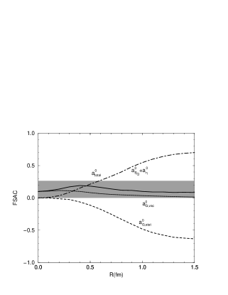
Figure 1: The flavor singlet axial current of the proton as a function of bag radius: (a) the quark and $\eta$ meson contribution $a_{B_{Q}}^{0}+a_{\eta}^{0}$, (b) the gluon contributions $a_{G,static}^{0}$ and $a_{G,vac}^{0}$ from static gluon due to quark source and gluon vacuum, respectively, (c) the total contribution $a_{total}^{0}$. The shaded area stands for the range admitted by experiments.

3 Baryon octet magnetic moments

3.1 Coleman-Glashow sum rules

Since Coleman and Glashow [177] predicted the magnetic moments of the baryon octet about forty years ago, there has been a lot of progress in both the theoretical paradigm and experimental verification for the baryon magnetic moments.

In this section, we will investigate the explicit Coleman-Glashow sum rules and spin symmetries of the magnetic moments of the baryon octet in the adjoint representation of the SU(3) flavor group by assuming that the chiral bag has the SU(3) flavor symmetry with $m_{u}=m_{d}=m_{s}$, $m_{\pi}=m_{K}$ and $f_{\pi}=f_{K}$. Even though the quark and pion masses in ${\cal L}_{CSB}$ in (2.2) break both the SU(3)${}_{L}\times$SU(3)_R and the diagonal SU(3) symmetry so that chiral symmetry cannot be conserved, these terms without derivatives yield no explicit contribution to the EM currents $J_{EM}^{\mu}$ obtainable from (2.6), and at least in the adjoint representation of the SU(3) group the EM currents are conserved and of the same form as the chiral limit result $J_{EM,CS}^{\mu}$ to preserve the U-spin symmetry.

The higher representation mixing in the baryon wave functions, induced by the different pseudoscalar meson masses and decay constants outside and different quark masses inside the bag, will be discussed in the next section in terms of the multiquark structure scheme where the chiral bag has additional meson contribution from the $\bar{\rm q}$q content inside the bag.

In the collective quantization scheme of the CBM which was discussed in the previous section, the EM currents yield the magnetic moment operators of the same form as the chiral symmetric limit consequence $\hat{\mu}_{CS}^{i}=\hat{\mu}_{CS}^{i(3)}+\frac{1}{\sqrt{3}}\hat{\mu}_{CS}^{i(8)}$ where

$$\hat{\mu}_{CS}^{i(a)}=-{\cal N}D_{ai}^{8}-{\cal N}^{\prime}d_{ipq}D_{ap}^{8}\hat{T}_{q}^{R}+\frac{N_{c}}{2\sqrt{3}}{\cal M}D_{a8}^{8}\hat{J}_{i}.$$ (3.1)

Here $\hat{J}_{i}=-\hat{T}_{i}^{R}$ are the SU(2) spin operators, and $\hat{T}_{i}^{R}$ and $\hat{T}_{p}^{R}$ are the right SU(3) isospin operators along the isospin and strangeness directions respectively, and the inertia parameters are of complicated forms given by

$${\cal N} = \frac{3}{2}\sum_{m}{\rm sgn}(\varepsilon_{m}){}_{h}\langle m|\mu_{3}^{(3)}|m\rangle_{h}-3\langle v|\mu_{3}^{(3)}|v\rangle$$

$$+\frac{4\pi}{3e^{3}f_{\pi}}\int_{ef_{\pi}R}^{\infty}{\rm d}zz^{2}\sin^{2}\theta\left[1+(\frac{d\theta}{dz})^{2}+\frac{\sin^{2}\theta}{z^{2}}\right]$$

$${\cal N}^{\prime} = -\frac{1}{{\cal I}_{2}}\frac{3}{2}\sum_{m,n}\left[\frac{{}_{h}\langle m|\lambda_{4}|n\rangle_{s}{}_{s}\langle n|\mu_{3}^{(4)}|m\rangle_{h}}{\varepsilon_{m}-\omega_{n}}+\frac{{}_{s}\langle m|\lambda_{4}|n\rangle_{h}{}_{h}\langle n|\mu_{3}^{(4)}|m\rangle_{s}}{\omega_{m}-\varepsilon_{n}}\right]$$

$$-\frac{1}{{\cal I}_{2}}\frac{3}{2}\sum_{m}\frac{\langle v|\lambda_{4}|m\rangle_{s}{}_{s}\langle m|\mu_{3}^{(4)}|v\rangle}{\omega_{m}-\varepsilon_{v}}+\frac{1}{3\pi e^{2}f_{\pi}^{2}}\int_{ef_{\pi}R}^{\infty}{\rm d}z~{}z^{2}\sin^{2}\theta\frac{d\theta}{dz}$$

$${\cal M} = -\frac{1}{{\cal I}_{1}}\frac{3}{2}\sum_{m,n}\frac{{}_{h}\langle m|\lambda_{3}|n\rangle_{h}{}_{h}\langle n|\mu_{3}^{(0)}|m\rangle_{h}}{\varepsilon_{m}-\varepsilon_{n}}-\frac{1}{{\cal I}_{1}}\frac{3}{2}\sum_{m}\frac{\langle v|\lambda_{3}|m\rangle_{h}{}_{h}\langle m|\mu_{3}^{(0)}|v\rangle}{\varepsilon_{m}-\varepsilon_{v}}$$ (3.2)

$$+\frac{1}{{\cal I}_{1}}\frac{1}{3\pi e^{2}f_{\pi}^{2}}\int_{ef_{\pi}R}^{\infty}{\rm d}z~{}z^{2}\sin^{2}\theta\frac{d\theta}{dz}$$

with $\mu_{3}^{(3)}=\frac{1}{4}\cdot\frac{1}{3}\vec{\lambda}\cdot\vec{V}$, $\mu_{3}^{(4)}=\frac{1}{4}V_{3}$ and $\mu_{3}^{(0)}=\frac{1}{4}\frac{2}{3}V_{3}$ where $V_{i}=\epsilon_{ijk}x_{j}\gamma^{0}\gamma^{k}$ and the hermitian conjugate matrix elements are understood in the quark phase parts of ${\cal N}^{\prime}$ and ${\cal M}$. The numerical values [35, 25] of these inertia parameters are summarized in Table 1 and their quark phase inertia parameters are discussed in Ref. [35] and Appendix B. Here one notes that ${\cal M}$ and ${\cal N}^{\prime}$ originate from the topological WZW term along the isospin and strangeness directions, respectively.

Table 1: The inertia parameters as a function of the bag radius $R$ with $f_{\pi}=93MeV$, $f_{K}=114MeV$ and $e=4.75$.

$R$	${\cal M}$	${\cal N}$	${\cal N}^{\prime}$	${\cal P}$	${\cal Q}$	$\omega$
0.00	0.671	5.028	0.908	0.762	0.986	5.372
0.10	0.671	5.088	0.835	0.772	1.000	6.008
0.20	0.669	5.371	0.791	0.822	1.062	7.144
0.30	0.660	5.660	0.752	0.886	1.125	8.290
0.40	0.647	5.697	0.699	0.944	1.159	8.991
0.50	0.643	5.834	0.615	1.022	1.205	10.133
0.60	0.656	6.000	0.519	1.112	1.265	11.875
0.70	0.693	6.128	0.424	1.184	1.305	14.022
0.80	0.768	6.167	0.335	1.212	1.302	16.550
0.90	0.886	6.130	0.266	1.185	1.249	19.280
1.00	1.042	6.056	0.222	1.114	1.156	21.987

With respect to the octet baryon wave function $\Phi_{B}^{\lambda}$ discussed in (2.33), the spectrum of the magnetic moment operator $\hat{\mu}^{i}$ in the adjoint representation of the SU(3) flavor symmetric limit has the following U-spin symmetric Coleman-Glashow sum rules [177, 178, 179] due to the degenerate d- and s-flavor charges in the SU(3) EM charge operator $\hat{Q}_{EM}$ in the EM currents

$$\mu_{\Sigma^{+}} = \mu_{p}=\frac{1}{10}{\cal M}+\frac{4}{15}({\cal N}+\frac{1}{2}{\cal N}^{\prime})$$

$$\mu_{\Xi^{0}} = \mu_{n}=\frac{1}{20}{\cal M}-\frac{1}{5}({\cal N}+\frac{1}{2}{\cal N}^{\prime})$$

$$\mu_{\Xi^{-}} = \mu_{\Sigma^{-}}=-\frac{3}{20}{\cal M}-\frac{1}{15}({\cal N}+\frac{1}{2}{\cal N}^{\prime})$$

$$\mu_{\Sigma^{0}} = -\mu_{\Lambda}=-\frac{1}{40}{\cal M}+\frac{1}{10}({\cal N}+\frac{1}{2}{\cal N}^{\prime}).$$ (3.3)

Here one should note that the U-spin symmetry originates from the SU(3) group theoretical fact that the matrix elements of the magnetic moment operators in (3.1) in the adjoint representation, such as $\langle 8|D_{38}^{8}+\frac{1}{\sqrt{3}}D_{88}^{8}|8\rangle$, have degenerate values for the U-spin multiplets ($p$, $\Sigma^{+}$), ($n$, $\Xi^{0}$) and ($\Xi^{-}$, $\Sigma^{-}$) with the same electric charges.

In (3.3) one can easily see that $\mu_{\Sigma}(I_{3})=\mu_{\Sigma^{0}}+I_{3}\Delta_{\mu_{\Sigma}}$ where $\Delta_{\mu_{\Sigma}}=\frac{1}{8}{\cal M}+\frac{1}{6}({\cal N}+\frac{1}{2}{\cal N}^{\prime})$ so that the summation $\mu_{\Sigma^{+}}+\mu_{\Sigma^{-}}$ is independent of the third component of the isospin $I_{3}$ so that one can obtain the other Coleman-Glashow sum rules [177, 178, 179, 180]

$$\mu_{\Sigma^{0}}=\frac{1}{2}(\mu_{\Sigma^{+}}+\mu_{\Sigma^{-}}).$$ (3.4)

Since there is no SU(3) singlet contribution to the magnetic moment, the summation of the magnetic moments over the octet baryon vanishes to yield the identity [179]

$$\sum_{B\in{\rm octet}}\mu_{B}=0.$$ (3.5)

Introducing in the meson pieces of the CBM Lagrangian (2.1) the minimal photon coupling to the derivative terms, $\partial_{\mu}U\rightarrow\nabla_{\mu}U=\partial_{\mu}U+ieA_{\mu}[\hat{Q}_{EM},U]$ with the SU(3) EM charge operator $\hat{Q}_{EM}$ one obtains the $\Lambda\Sigma^{0}$ transition matrix element for the decay $\Sigma^{0}\rightarrow\Lambda+\gamma$

$$\frac{1}{\sqrt{3}}\mu_{\Lambda\Sigma^{0}}=-\frac{1}{40}{\cal M}+\frac{1}{10}({\cal M}+\frac{1}{2}{\cal N}^{\prime})$$ (3.6)

which, in incorporating an SU(3) singlet contribution of the photon, satisfies the modified Coleman-Glashow sum rules [180, 181]

$$\frac{1}{\sqrt{3}}\mu_{\Lambda\Sigma^{0}} = \mu_{\Lambda}-\mu_{n}$$

$$\frac{6}{\sqrt{3}}\mu_{\Lambda\Sigma^{0}} = \mu_{\Sigma^{0}}-2\mu_{\Xi^{0}}+3\mu_{\Lambda}-2\mu_{n}.$$ (3.7)

It is also interesting to note that the hyperon and transition magnetic moments in the SU(3) flavor symmetric limit can be expressed in terms of the nucleon magnetic moments only [177, 178, 182]

$$\mu_{\Lambda}=\frac{1}{2}\mu_{n}$$

$$\mu_{\Xi^{-}}=-(\mu_{p}+\mu_{n})$$

$$\mu_{\Sigma^{+}}-\mu_{\Sigma^{-}}+\mu_{\Xi^{0}}-\mu_{\Xi^{-}}=3(\mu_{p}+\mu_{n})$$

$$\frac{1}{\sqrt{3}}\mu_{\Lambda\Sigma^{0}}=-\frac{1}{2}\mu_{n}.$$ (3.8)

Here one should note that the transition magnetic moment possesses an arbitrary global phase factor in itself, while the other octet magnetic moments have a definite overall sign. In (3.8) we have used the phase convention of Ref. [183], which is consistent with de Swart convention [184] of the SU(3) isoscalar factors used in the CBM.

3.2 Strangeness in Yabu-Ando scheme

In the previous section we have considered the CBM in the adjoint representation with the SU(3) flavor symmetry, where the U-spin symmetry is conserved even though we have the chiral symmetry breaking mass terms. Now we include the SU(3) flavor symmetry breaking terms ${\cal L}_{FSB}$ in (2.2) to yield the magnetic moment operators $\hat{\mu}_{FSB}^{i(a)}$ of (3.9) induced by the symmetry breaking kinetic terms. However, the symmetry is also broken nonperturbatively by the mass terms via the higher dimensional IR channels where the CBM can be treated in the Yabu-Ando scheme [82] to yield the multiquark structure with the meson cloud ${\it inside}$ the bag. The quantum mechanical perturbative scheme to the symmetry breaking effects in the multiquark structure will be discussed in terms of the V-spin symmetry in the next section.

Assuming that the CBM includes the kinetic term in ${\cal L}_{FSB}$ in the collective quantization, the Noether scheme gives rise to the U-spin symmetry breaking conserved EM currents $J_{EM,FSB}^{\mu}$ so that $J_{EM}^{\mu}=J_{EM,CS}^{\mu}+J_{EM,FSB}^{\mu}$. With the spinning CBM ansatz the EM currents yield the magnetic moment operators $\hat{\mu}^{i}=\hat{\mu}^{i(3)}+\frac{1}{\sqrt{3}}\hat{\mu}^{i(8)}$ where $\hat{\mu}^{i(a)}=\hat{\mu}_{CS}^{i(a)}+\hat{\mu}_{FSB}^{i(a)}$. Here $\hat{\mu}_{CS}^{i(a)}$ is given in (3.1) and $\hat{\mu}_{FSB}^{i(a)}$ is described as below

$$\hat{\mu}^{i(a)}_{FSB}=-{\cal P}D_{ai}^{8}(1-D_{88}^{8})+\frac{\sqrt{3}}{2}{\cal Q}d_{ipq}D_{ap}^{8}D_{8q}^{8}$$ (3.9)

where ${\cal P}$ and ${\cal Q}$ are the inertia parameters along the isospin and strangeness directions obtained from the mesonic Lagrangian ${\cal L}_{FSB}$

$${\cal P} = \frac{8\pi}{9e^{3}f_{\pi}^{3}}(f_{K}^{2}-f_{\pi}^{2})\int_{ef_{\pi}R}^{\infty}{\rm d}zz^{2}\sin^{2}\theta\cos\theta$$

$${\cal Q} = \frac{8\pi}{9e^{3}f_{\pi}^{3}}(f_{K}^{2}-f_{\pi}^{2})\int_{ef_{\pi}R}^{\infty}{\rm d}zz^{2}\sin^{2}\theta$$

$$m{\cal I}_{2} = \frac{8\pi}{3e^{3}f_{\pi}^{3}}(f_{K}^{2}m_{K}^{2}-f_{\pi}^{2}m_{\pi}^{2})\int_{ef_{\pi}R}^{\infty}{\rm d}zz^{2}(1-\cos\theta)$$ (3.10)

$$+\frac{4\pi}{3ef_{\pi}}(f_{K}^{2}-f_{\pi}^{2})\int_{ef_{\pi}R}^{\infty}{\rm d}zz^{2}\left(\left(\frac{{\rm d}\theta}{{\rm d}z}\right)^{2}+\frac{2\sin^{2}\theta}{z^{2}}\right)\cos\theta$$

$$+\frac{1}{3}m_{s}N_{c}\sum_{n}{}_{h}\langle n|\gamma^{0}|n\rangle_{h}$$

whose numerical values are shown in Table 1.

Breaking up the tensor product of the Wigner $D$ functions into a sum of the single $D$ functions [184],

$$D_{a_{1}b_{1}}^{8}D_{a_{2}b_{2}}^{8}=\sum_{a,b,\lambda,\gamma}\left(\begin{array}[]{ccc}8&8&\lambda_{\gamma}\\ a_{1}&a_{2}&a\end{array}\right)\left(\begin{array}[]{ccc}8&8&\lambda_{\gamma}\\ b_{1}&b_{2}&b\end{array}\right)D_{ab}^{\lambda},$$ (3.11)

one can rewrite the isovector and isoscalar parts of the operator $\hat{\mu}_{FSB}^{i(a)}$ as

$$\hat{\mu}^{i(3)}_{FSB} = {\cal P}(-\frac{4}{5}D_{3i}^{8}+\frac{1}{4}(D_{3i}^{10}+D_{3i}^{\bar{10}})+\frac{3}{10}D_{3i}^{27})+{\cal Q}(\frac{3}{10}D_{3i}^{8}-\frac{3}{10}D_{3i}^{27})$$

$$\hat{\mu}^{i(8)}_{FSB} = {\cal P}(-\frac{6}{5}D_{8i}^{8}+\frac{9}{20}D_{8i}^{27})+{\cal Q}(-\frac{3}{10}D_{8i}^{8}-\frac{9}{20}D_{8i}^{27}).$$ (3.12)

Here the ${\bf 10}$ and $\bar{\bf 10}$ IRs, which are absent in the isoscalar channel due to their nonvanishing hypercharge, come out together to conserve the hermitian property of the operator in the isovector channel, while the singlet operator constructed in the singlet IR ${\bf 1}$ cannot allow the quantum number ($Y_{R}$;$J$,-$J_{3}$)=(0;1,0) [179] so that the operator does not occur in either channel.

Using the octet baryon wave function (2.33) for the matrix elements of the full magnetic moment operator $\hat{\mu}^{i}$, one can obtain the hyperfine structure in the adjoint representation

$$\mu_{p} = \frac{1}{10}{\cal M}+\frac{4}{15}({\cal N}+\frac{1}{2}{\cal N}^{\prime})+\frac{8}{45}{\cal P}-\frac{2}{45}{\cal Q}$$

$$\mu_{n} = \frac{1}{20}{\cal M}-\frac{1}{5}({\cal N}+\frac{1}{2}{\cal N}^{\prime})-\frac{1}{9}{\cal P}+\frac{7}{90}{\cal Q}$$

$$\mu_{\Lambda} = \frac{1}{40}{\cal M}-\frac{1}{10}({\cal N}+\frac{1}{2}{\cal N}^{\prime})-\frac{1}{10}{\cal P}-\frac{1}{20}{\cal Q}$$

$$\mu_{\Xi^{0}} = \frac{1}{20}{\cal M}-\frac{1}{5}({\cal N}+\frac{1}{2}{\cal N}^{\prime})-\frac{11}{45}{\cal P}-\frac{1}{45}{\cal Q}$$

$$\mu_{\Xi^{-}} = -\frac{3}{20}{\cal M}-\frac{1}{15}({\cal N}+\frac{1}{2}{\cal N}^{\prime})-\frac{4}{45}{\cal P}-\frac{2}{45}{\cal Q}$$

$$\mu_{\Sigma^{+}} = \frac{1}{10}{\cal M}+\frac{4}{15}({\cal N}+\frac{1}{2}{\cal N}^{\prime})+\frac{13}{45}{\cal P}-\frac{1}{45}{\cal Q}$$

$$\mu_{\Sigma^{0}} = -\frac{1}{40}{\cal M}+\frac{1}{10}({\cal N}+\frac{1}{2}{\cal N}^{\prime})+\frac{11}{90}{\cal P}+\frac{1}{36}{\cal Q}$$

$$\mu_{\Sigma^{-}} = -\frac{3}{20}{\cal M}-\frac{1}{15}({\cal N}+\frac{1}{2}{\cal N}^{\prime})-\frac{2}{45}{\cal P}+\frac{7}{90}{\cal Q}.$$ (3.13)

Here one notes that the Coleman-Glashow sum rules (3.4) and (3.5) are still valid while the other relations (3.3) and(3.8) are no longer retained due to the SU(3) flavor symmetry breaking effects of $m_{u}=m_{d}\neq m_{s}$, $m_{\pi}\neq m_{K}$ and $f_{\pi}\neq f_{K}$ through the inertia parameters ${\cal P}$ and ${\cal Q}$.

By substituting the EM charge operator $\hat{Q}_{EM}$ with the q-flavor EM charge operator $\hat{Q}_{q}$, one can obtain the q-flavor currents $J_{EM}^{\mu(q)}=J_{EM,CS}^{\mu(q)}+J_{EM,FSB}^{\mu(q)}$ in the SU(3) flavor symmetry broken case to yield the EM currents with three flavor pieces $J_{EM}^{\mu}=J_{EM}^{\mu(u)}+J_{EM}^{\mu(d)}+J_{EM}^{\mu(s)}$. Here one notes that by defining the flavor projection operators

$$\hat{P}_{u} = \frac{1}{3}+\frac{1}{2}\lambda_{3}+\frac{1}{2\sqrt{3}}\lambda_{8},$$

$$\hat{P}_{d} = \frac{1}{3}-\frac{1}{2}\lambda_{3}+\frac{1}{2\sqrt{3}}\lambda_{8},$$

$$\hat{P}_{s} = \frac{1}{3}-\frac{1}{2\sqrt{3}}\lambda_{8},$$ (3.14)

satisfying $\hat{P}_{q}^{2}=\hat{P}_{q}$ and $\sum_{q}\hat{P}_{q}=1$, one can easily construct the q-flavor EM charge operators $\hat{Q}_{q}=\hat{Q}_{EM}\hat{P}_{q}=Q_{q}\hat{P}_{q}$.

As in the previous section, one can then find the magnetic moment operator in the u-flavor channel

$$\hat{\mu}^{i(u)} = {\cal M}\frac{2N_{c}}{9}(1+\frac{\sqrt{3}}{2}D_{38}^{8}+\frac{1}{2}D_{88}^{8})\hat{J}_{i}-{\cal N}\frac{2}{3}(D_{3i}^{8}+\frac{1}{\sqrt{3}}D_{8i}^{8})$$ (3.15)

$$-{\cal N}^{\prime}\frac{2}{3}d_{ipq}(D_{3p}^{8}+\frac{1}{\sqrt{3}}D_{8p}^{8})\hat{T}_{q}^{R}-{\cal P}\frac{2}{3}(D_{3i}^{8}+\frac{1}{\sqrt{3}}D_{8i}^{8})(1-D_{88}^{8})$$

$$+{\cal Q}\frac{1}{\sqrt{3}}d_{ipq}(D_{3p}^{8}+\frac{1}{\sqrt{3}}D_{8p}^{8})D_{8q}^{8}$$

to yield the u-components of the baryon octet magnetic moments in the adjoint representation

$$\mu_{p}^{(u)} = \frac{2}{510}{\cal M}+\frac{8}{45}({\cal N}+\frac{1}{2}{\cal N}^{\prime})+\frac{16}{135}{\cal P}-\frac{4}{135}{\cal Q}$$

$$\mu_{n}^{(u)} = \frac{11}{30}{\cal M}-\frac{2}{15}({\cal N}+\frac{1}{2}{\cal N}^{\prime})-\frac{2}{27}{\cal P}+\frac{7}{135}{\cal Q}$$

$$\mu_{\Lambda}^{(u)} = \frac{7}{20}{\cal M}-\frac{1}{15}({\cal N}+\frac{1}{2}{\cal N}^{\prime})-\frac{1}{15}{\cal P}-\frac{1}{30}{\cal Q}$$

$$\mu_{\Xi^{0}}^{(u)} = \frac{11}{30}{\cal M}-\frac{2}{15}({\cal N}+\frac{1}{2}{\cal N}^{\prime})-\frac{22}{135}{\cal P}-\frac{2}{135}{\cal Q}$$

$$\mu_{\Xi^{-}}^{(u)} = \frac{7}{30}{\cal M}-\frac{1}{45}({\cal N}+\frac{1}{2}{\cal N}^{\prime})-\frac{8}{135}{\cal P}-\frac{4}{135}{\cal Q}$$

$$\mu_{\Sigma^{+}}^{(u)} = \frac{2}{5}{\cal M}+\frac{8}{45}({\cal N}+\frac{1}{2}{\cal N}^{\prime})+\frac{26}{135}{\cal P}-\frac{2}{135}{\cal Q}$$

$$\mu_{\Sigma^{0}}^{(u)} = \frac{19}{60}{\cal M}+\frac{1}{15}({\cal N}+\frac{1}{2}{\cal N}^{\prime})+\frac{11}{135}{\cal P}+\frac{1}{54}{\cal Q}$$

$$\mu_{\Sigma^{-}}^{(u)} = \frac{7}{30}{\cal M}-\frac{2}{45}({\cal N}+\frac{1}{2}{\cal N}^{\prime})-\frac{4}{135}{\cal P}+\frac{7}{135}{\cal Q}.$$ (3.16)

Similarly one can construct the s-flavor magnetic moment operator

$$\hat{\mu}^{i(s)} = -{\cal M}\frac{N_{c}}{9}(1-D_{88}^{8})\hat{J}_{i}-{\cal N}\frac{2}{3\sqrt{3}}D_{8i}^{8}-{\cal N}^{\prime}\frac{2}{3\sqrt{3}}d_{ipq}D_{8p}^{8}\hat{T}_{q}^{R}$$ (3.17)

$$-{\cal P}\frac{2}{3\sqrt{3}}D_{8i}^{8}(1-D_{88}^{8})+{\cal Q}\frac{1}{3}d_{ipq}D_{8p}^{8}D_{8q}^{8}$$

to obtain the baryon octet magnetic moments in the s-flavor channel

$$\mu_{N}^{(s)} = -\frac{7}{60}{\cal M}+\frac{1}{45}({\cal N}+\frac{1}{2}{\cal N}^{\prime})+\frac{1}{45}{\cal P}+\frac{1}{90}{\cal Q}$$

$$\mu_{\Lambda}^{(s)} = -\frac{3}{20}{\cal M}-\frac{1}{15}({\cal N}+\frac{1}{2}{\cal N}^{\prime})-\frac{1}{15}{\cal P}-\frac{1}{30}{\cal Q}$$

$$\mu_{\Xi}^{(s)} = -\frac{11}{530}{\cal M}-\frac{42}{415}({\cal N}+\frac{1}{2}{\cal N}^{\prime})-\frac{122}{9135}{\cal P}-\frac{12}{4135}{\cal Q}$$

$$\mu_{\Sigma}^{(s)} = -\frac{11}{60}{\cal M}+\frac{1}{15}({\cal N}+\frac{1}{2}{\cal N}^{\prime})+\frac{11}{135}{\cal P}+\frac{1}{54}{\cal Q}.$$ (3.18)

Here one notes that all the baryon magnetic moments satisfy the model-independent relations in the u- and d-channels and the I-spin symmetry in the s-flavor channel where the isomultiplets have the same strangeness number

$$\mu_{B}^{(d)} = \frac{Q^{d}}{Q^{u}}\mu_{B}^{(u)}$$ (3.19)

$$\mu_{B}^{(s)} = \mu_{\bar{B}}^{(s)}.$$ (3.20)

Here $\bar{B}$ is the isospin conjugate baryon in the isomultiplets of the baryon.

For the $\Lambda\Sigma^{0}$ transition, one can obtain the u- and d-flavor components given by the different pattern

$$\frac{1}{\sqrt{3}}\mu_{\Lambda\Sigma^{0}}^{(u)}=\frac{2}{\sqrt{3}}\mu_{\Lambda\Sigma^{0}}^{(d)}=-\frac{1}{60}{\cal M}+\frac{1}{15}({\cal N}+\frac{1}{2}{\cal N}^{\prime})+\frac{8}{135}{\cal P}-\frac{7}{270}{\cal Q},$$ (3.21)

and the vanishing s-flavor component.

Until now we have considered the explicit SU(3) flavor symmetry breaking effects in the magnetic moment operators $\hat{\mu}^{i}$ of the CBM in the adjoint representation, where the mass terms in ${\cal L}_{CSB}$ and ${\cal L}_{FSB}$ cannot contribute to $\hat{\mu}^{i}$ due to the absence of the derivative term. Treating the mass terms as the representation dependent fraction in the Hamiltonian approach, one can see that the term with $D_{88}^{8}$ induces the representation mixing effects in the baryon wave functions. In order to investigate explicitly the mixing effects in the Yabu-Ando scheme, we quantize the collective variables $A(t)$ so that we can obtain the Hamiltonian of the form

$$H=M+\frac{1}{2}\left(\frac{1}{{\cal I}_{1}}-\frac{1}{{\cal I}_{2}}\right)\hat{J}^{2}+\frac{1}{2{\cal I}_{2}}\left(h_{SB}-\frac{3}{4}\hat{Y}_{R}^{2}\right)$$ (3.22)

where ${\cal I}_{1}$ and ${\cal I}_{2}$ are the moments of inertia of the CBM along the isospin and the strangeness directions respectively and their explicit expressions are given in (2.40).

Here one remembers that the static mass $M$ obtainable from (2.20) satisfies the equation of motion for the chiral angle (2.21). The pion mass in (2.21) also yields deviation from the chiral limit chiral angle for a fixed bag radius so that the numerical results in the massive CBM can be worsened when one uses the experimental decay constant.

In order to obtain the numerical results in Table 1, we use the massless chiral angle and the experimental data $f_{\pi}=93$ MeV, $f_{K}=114$ MeV and $e=4.75$ since $(m_{u}+m_{d})/m_{s}\approx m_{\pi}^{2}/m_{K}^{2}\approx 0.1$, so that we can neglect the light quark and pion masses. This approximation would not be contradictory to our main purpose to investigate the massive kaon contributions to the baryon magnetic moments.

On the other hand, the chiral and SU(3) flavor symmetry breaking induces the representation dependent part

$$h_{SB}=\hat{C}_{2}^{2}+\frac{2}{3}\omega(1-D_{88}^{8}),$$ (3.23)

where $\hat{C}_{2}^{2}$ is the Casimir operator in the SU(3)_L group and the symmetry breaking strength is given by

$$\omega = \frac{8\pi}{e^{3}f_{\pi}^{3}}{\cal I}_{2}(f_{K}^{2}m_{K}^{2}-f_{\pi}^{2}m_{\pi}^{2})\int_{ef_{\pi}R}^{\infty}{\rm d}zz^{2}(1-\cos\theta)+{\cal I}_{2}m_{s}N_{c}\sum_{n}\langle n|\gamma^{0}|n\rangle_{h}$$ (3.24)

$$+\frac{4\pi}{ef_{\pi}}{\cal I}_{2}(f_{K}^{2}-f_{\pi}^{2})\int_{ef_{\pi}R}^{\infty}{\rm d}zz^{2}\left(\left(\frac{d\theta}{dz}\right)^{2}+\frac{2\sin^{2}\theta}{z^{2}}\right)\cos\theta$$

with the numerical values in Table 1. Of course one can easily see that, in the vanishing $\omega$ limit, the Hamiltonian (3.22) approaches to the previous one $H_{0}$ in (2.41) with the SU(3) flavor symmetry.

Now one can directly diagonalize the Hamiltonian $h_{SB}$ in the eigenvalue equation $h_{SB}|B\rangle=\varepsilon_{SB}|B\rangle$ of the Yabu-Ando scheme [82] with the eigenstate denoted by $|B\rangle=\sum_{\lambda}C_{\lambda}^{B}|B\rangle^{\lambda}$ where $C_{\lambda}^{B}$ is the representation mixing coefficient and $|B\rangle$ are octet baryon wave function in the $\lambda$ dimensional IR discussed in (2.32).

Table 2: The baryon octet magnetic moments in the U-spin symmetry broken case in the Yabu-Ando scheme of the CBM, compared with the SU(2) CBM and naive NRQM predictions and the experimental data

R	$\mu_{p}$	$\mu_{n}$	$\mu_{\Lambda}$	$\mu_{\Xi^{0}}$	$\mu_{\Xi^{-}}$	$\mu_{\Sigma^{+}}$	$\mu_{\Sigma^{0}}$	$\mu_{\Sigma^{-}}$	$\mu_{\Lambda\Sigma^{0}}$
0.00	1.69	$-1.28$	$-0.56$	$-1.22$	$-0.47$	1.73	0.69	$-0.36$	1.19
0.10	1.71	$-1.30$	$-0.56$	$-1.22$	$-0.46$	1.73	0.69	$-0.36$	1.20
0.20	1.80	$-1.39$	$-0.56$	$-1.27$	$-0.45$	1.80	0.72	$-0.36$	1.28
0.30	1.89	$-1.48$	$-0.58$	$-1.32$	$-0.45$	1.86	0.75	$-0.36$	1.36
0.40	1.91	$-1.50$	$-0.57$	$-1.33$	$-0.44$	1.87	0.76	$-0.35$	1.38
0.50	1.96	$-1.54$	$-0.57$	$-1.36$	$-0.42$	1.89	0.77	$-0.35$	1.43
0.60	2.02	$-1.59$	$-0.57$	$-1.38$	$-0.40$	1.90	0.78	$-0.34$	1.48
0.70	2.07	$-1.62$	$-0.55$	$-1.39$	$-0.37$	1.89	0.78	$-0.34$	1.52
0.80	2.10	$-1.62$	$-0.53$	$-1.37$	$-0.34$	1.85	0.76	$-0.34$	1.51
0.90	2.10	$-1.59$	$-0.49$	$-1.33$	$-0.31$	1.79	0.73	$-0.34$	1.48
1.00	2.10	$-1.55$	$-0.45$	$-1.26$	$-0.28$	1.73	0.69	$-0.35$	1.26
${\rm SU(2)}$	2.27	$-1.35$	$-0.61$	$-1.33$	$-0.60$	2.28	0.82	$-0.64$	1.26
${\rm naive}$	2.79	$-1.86$	$-0.61$	$-1.43$	$-0.50$	2.68	0.82	$-1.04$	1.61
${\rm exp}$	2.79	$-1.91$	$-0.61$	$-1.25$	$-0.65$	2.46	$-$	$-1.16$	1.61

The possible SU(3) representations of the minimal multiquark Fock space qqq+qqq$\bar{\rm q}$q are restricted by the Clebsch-Gordan series ${\bf 8}\oplus\bar{\bf 10}\oplus{\bf 27}$ in the baryon octet with $Y_{R}=1$ and $J=\frac{1}{2}$, so that the representation mixing coefficients can be evaluated by solving the eigenvalue equation of the 3$\times$3 Hamiltonian matrix in (3.22).

Since in the multiquark scheme of the CBM the baryon wave functions act nonperturbatively on the magnetic moment operators with the quark and meson phase contributions in their inertia parameters, one could have the meson cloud content $\bar{\rm q}$q inside the bag via the channel of qqq$\bar{\rm q}$q multiquark Fock space. Here in order to construct the pseudoscalar mesons inside the bag, the $\bar{\rm q}$q contents refer to all the appropriate flavor combinations.

In the SU(3) flavor sector of the CBM, the mechanism explaining the meson cloud inside the bag surface seems [37] closely related to the pseudoscalar composite operators $\bar{\psi}i\gamma_{5}\lambda_{a}\psi\sim\pi_{a}$ ($a=1,...,8$) since the pseudoscalar quark bilinears transform like $({\bf 3},\bar{\bf 3})\oplus(\bar{\bf 3},{\bf 3})$, while in the U(1) flavor sector the mechanism is supposed [37] to be described with the anomalous gluon effect in the quark-antiquark annihilation channel [185]. In the SU(3) CBM with the minimal multiquark Fock space, the meson cloud content $\bar{\rm q}$q inside the bag surface can be then phenomenologically illustrated [37] by sum of two topologically different Feynman diagrams. One notes here that, in the multiquark scheme of the SU(3) CBM, the baryon magnetic moments have two-body operator effect as well as one-body self interaction in the sense of quasi-particle model in the many body problem. The gluons are supposed to mediate the pseudoscalar $\eta_{0}$ meson cloud via the $\bar{\rm q}$q pair creation and annihilation process.

As shown in Table 2, the U-spin symmetry breaking effect, through the explicit operator $\hat{\mu}_{FSB}^{i(a)}$ and the Yabu-Ando scheme in the multiquark structure, improves the fit to most of the baryon octet magnetic moments. However if the experimental data [186] is correct, the fit to the $\mu_{\Sigma^{-}}$ seems a little bit worsened. Here one should note that $\mu_{\Lambda}$ seems to be well predicted in the CBM as in the naive NRQM since $\mu_{\Lambda}$ could be mainly determined from the strange quark and kaon whose masses are kept in our massless profile approximation. From the numerical values in Table 2, one can see that the SU(3) CBM could be regarded to be a good candidate of the unification of the bag and Skyrmion models with predictions almost independent of the bag radius. For the $\Sigma^{0}\rightarrow\Lambda+\gamma$ transition matrix element, we obtain the numerical prediction of the CBM $\mu_{\Lambda\Sigma^{0}}=1.19-1.53$ comparable to the experimental data $\mu_{\Lambda\Sigma^{0}}^{exp}=1.61$ [186].

In the q-flavor channels, the I-spin symmetry and model-independent relations (3.20) hold in the multiquark scheme since the Hamiltonian $h_{SB}$ has the eigenstates degenerate with the isomultiplets in our approximation, where the I-spin symmetry breaking light quark masses are neglected.

4 Baryon decuplet magnetic moments

4.1 Model-independent sum rules

In the previous section we have calculated the magnetic moments of baryon octet in the SU(3) flavor case [37], where the Coleman-Glashow sum rules [174] including the U-spin symmetry hold up to the SU(3) flavor symmetric limit of the adjoint representation to suggest the possibility of a unification of the SU(3) CBM and the naive NRQM. The measurements of the magnetic moments of the decuplet baryons were reported for $\mu_{\Delta^{++}}$ [187] and $\mu_{\Omega^{-}}$ [188] to yield a new avenue for understanding hadronic structure.

In this section we will calculate the magnetic moments of the baryon decuplet [38] to compare with the known experimental data, to make new predictions in the CBM for the unknown experiments and to derive the model-independent sum rules which will be used later to generalize the CBM conjecture [37] for the baryon decuplet.

In order to estimate the magnetic moments of the decuplet baryons in the U-spin broken symmetry case, we have at first derived the explicit magnetic moment operators $\hat{\mu}_{FSB}^{i(a)}$ from the flavor symmetry breaking Lagrangian ${\cal L}_{FSB}$ in the adjoint representation where $\hat{\mu}_{CSB}^{i(a)}$ vanishes. In the SU(3) cranking scheme described in the previous sections, the magnetic moment operators $\hat{\mu}^{i}$ are then given by (3.1) and (3.9) and the tensor product of the Wigner $D$ functions in $\hat{\mu}_{FSB}^{i(a)}$ can be decomposed into a sum of the single $D$ functions to yield the isovector and isoscalar parts as below

$$\hat{\mu}^{i(3)}_{FSB} = {\cal P}(-\frac{4}{5}D_{3i}^{8}+\frac{3}{10}D_{3i}^{27})+{\cal Q}(\frac{3}{10}D_{3i}^{8}-\frac{3}{10}D_{3i}^{27})$$

$$\hat{\mu}^{i(8)}_{FSB} = {\cal P}(-\frac{6}{5}D_{8i}^{8}+\frac{9}{20}D_{8i}^{27})+{\cal Q}(-\frac{3}{10}D_{8i}^{8}-\frac{9}{20}D_{8i}^{27}).$$ (4.1)

Here one notes that, to conserve the hermitian property of the magnetic moment operator, ${\bf 10}$ and $\bar{\bf 10}$ IRs appear together in the isovector channel of the baryon octet as discussed in the previous section while the ${\bf 1}$, ${\bf 10}$ and $\bar{{\bf 10}}$ IRs do not take place in the decuplet baryons.

With respect to the decuplet baryon wave function $\Phi_{B}^{\lambda}$ in (2.33) the magnetic moment operator $\hat{\mu}^{i}$ has the spectrum for the decuplet in the adjoint representation

$$\mu_{\Delta^{++}} = \frac{1}{8}{\cal M}+\frac{1}{2}({\cal N}-\frac{1}{2\sqrt{3}}{\cal N}^{\prime})+\frac{3}{7}{\cal P}-\frac{3}{56}{\cal Q}$$

$$\mu_{\Delta^{+}} = \frac{1}{16}{\cal M}+\frac{1}{4}({\cal N}-\frac{1}{2\sqrt{3}}{\cal N}^{\prime})+\frac{5}{21}{\cal P}+\frac{1}{84}{\cal Q}$$

$$\mu_{\Delta^{0}} = \frac{1}{21}{\cal P}+\frac{13}{168}{\cal Q}$$

$$\mu_{\Delta^{-}} = -\frac{1}{16}{\cal M}-\frac{1}{4}({\cal N}-\frac{1}{2\sqrt{3}}{\cal N}^{\prime})-\frac{1}{7}{\cal P}+\frac{1}{7}{\cal Q}$$

$$\mu_{\Sigma^{*+}} = \frac{1}{16}{\cal M}+\frac{1}{4}({\cal N}-\frac{1}{2\sqrt{3}}{\cal N}^{\prime})+\frac{19}{84}{\cal P}-\frac{17}{168}{\cal Q}$$

$$\mu_{\Sigma^{*0}} = \frac{1}{84}{\cal P}-\frac{1}{84}{\cal Q}$$

$$\mu_{\Sigma^{*-}} = -\frac{1}{16}{\cal M}-\frac{1}{4}({\cal N}-\frac{1}{2\sqrt{3}}{\cal N}^{\prime})-\frac{17}{84}{\cal P}+\frac{13}{168}{\cal Q}$$

$$\mu_{\Xi^{*0}} = -\frac{1}{42}{\cal P}-\frac{17}{168}{\cal Q}$$

$$\mu_{\Xi^{*-}} = -\frac{1}{16}{\cal M}-\frac{1}{4}({\cal N}-\frac{1}{2\sqrt{3}}{\cal N}^{\prime})-\frac{11}{42}{\cal P}+\frac{1}{84}{\cal Q}$$

$$\mu_{\Omega^{-}} = -\frac{1}{16}{\cal M}-\frac{1}{4}({\cal N}-\frac{1}{2\sqrt{3}}{\cal N}^{\prime})-\frac{9}{28}{\cal P}-\frac{3}{56}{\cal Q}.$$ (4.2)

In the SU(3) flavor symmetric limit with the chiral symmetry breaking masses $m_{u}=m_{d}=m_{s}$, $m_{K}=m_{\pi}$ and decay constants $f_{K}=f_{\pi}$, the magnetic moments of the decuplet baryons are simply given by [189]

$$\mu_{B}=Q_{EM}(\frac{1}{16}{\cal M}+\frac{1}{4}({\cal N}-\frac{1}{2\sqrt{3}}{\cal N}^{\prime}))$$ (4.3)

where $Q_{EM}$ is the EM charge. Here one remembers that for the case of the CBM in the adjoint representation, the prediction of the baryon magnetic moments with the chiral symmetry is the same as that with the SU(3) flavor symmetry since the mass-dependent term in ${\cal L}_{CSB}$ and ${\cal L}_{FSB}$ do not yield any contribution to $J^{\mu}_{FSB}$ so that there is no terms with ${\cal P}$ and ${\cal Q}$ in (4.2).

Due to the degenerate d- and s-flavor charges in the SU(3) EM charge operator $\hat{Q}_{EM}$, the CBM possesses the generalized U-spin symmetry relations in the baryon decuplet magnetic moments, similar to those in the octet baryons (3.3),

$$\mu_{\Delta^{-}} = \mu_{\Sigma^{*-}}=\mu_{\Xi^{*-}}=\mu_{\Omega^{-}}$$

$$\mu_{\Delta^{0}} = \mu_{\Sigma^{*0}}=\mu_{\Xi^{*0}}$$

$$\mu_{\Delta^{+}} = \mu_{\Sigma^{*+}}$$ (4.4)

which will be shown to be shared with the naive NRQM, to support the effective NRQM conjecture of the CBM.

Since the SU(3) FSB quark masses do not affect the magnetic moments of the baryon decuplet in the ${\it adjoint}$ representation of the CBM, in the more general SU(3) flavor symmetry broken case with $m_{u}=m_{d}\neq m_{s}$, $m_{\pi}\neq m_{K}$ and $f_{\pi}\neq f_{K}$, the decuplet baryon magnetic moments with ${\cal P}$ and ${\cal Q}$ satisfy the other sum rules [38]

$$\mu_{\Sigma^{*0}} = \frac{1}{2}(\mu_{\Sigma^{*+}}+\mu_{\Sigma^{*-}})$$ (4.5)

$$\mu_{\Delta^{-}}+\mu_{\Delta^{++}} = \mu_{\Delta^{0}}+\mu_{\Delta^{+}}$$ (4.6)

$$\sum_{B\in{\rm decuplet}}\mu_{B} = 0.$$ (4.7)

Here one notes that the $\Sigma^{*}$ hyperons satisfy the identity $\mu_{\Sigma^{*}}(I_{3})=\mu_{\Sigma^{*0}}+I_{3}\Delta\mu_{\Sigma^{*}}$, where $\Delta\mu_{\Sigma^{*}}=\frac{1}{16}{\cal M}+\frac{1}{4}({\cal N}-\frac{1}{2\sqrt{3}}{\cal N}^{\prime})+\frac{3}{14}{\cal P}-\frac{5}{56}{\cal Q}$, such that $\mu_{\Sigma^{*+}}+\mu_{\Sigma^{*-}}$ is independent of $I_{3}$ as in (4.5). For the $\Delta$ baryons one can formulate the relation $\mu_{\Delta}(I_{3})=\mu_{\Delta}^{0}+I_{3}\Delta\mu_{\Delta}$ with $\mu_{\Delta}^{0}=\frac{1}{32}{\cal M}+\frac{1}{8}({\cal N}-\frac{1}{2\sqrt{3}}{\cal N}^{\prime})+\frac{1}{7}{\cal P}+\frac{5}{112}{\cal Q}$ and $\Delta\mu_{\Delta}=\frac{1}{16}{\cal M}+\frac{1}{4}({\cal N}-\frac{1}{2\sqrt{3}}{\cal N}^{\prime})+\frac{4}{21}{\cal P}-\frac{11}{168}{\cal Q}$, so that $\Delta$ baryons can be easily seen to fulfill the sum rule (4.6). Also the summation of the magnetic moments over all the decuplet baryons vanish to yield the model independent relation (4.7). Also the summation of the magnetic moments over all the decuplet baryons vanishes to yield the model independent relation, namely the third sum rule in (4.7), since there is no SU(3) singlet contribution to the magnetic moments as in the baryon octet magnetic moments.

In the SU(3) flavor symmetry broken case, by using the projection operators in (3.14) we can decompose the EM currents into three flavor pieces to obtain the baryon decuplet magnetic moments in the u-flavor channels of the adjoint representation

$$\mu_{\Delta^{++}}^{(u)} = \frac{5}{12}{\cal M}+\frac{1}{3}({\cal N}-\frac{1}{2\sqrt{3}}{\cal N}^{\prime})+\frac{2}{7}{\cal P}-\frac{1}{28}{\cal Q}$$

$$\mu_{\Delta^{+}}^{(u)} = \frac{3}{8}{\cal M}+\frac{1}{6}({\cal N}-\frac{1}{2\sqrt{3}}{\cal N}^{\prime})+\frac{10}{63}{\cal P}+\frac{1}{126}{\cal Q}$$

$$\mu_{\Delta^{0}}^{(u)} = \frac{1}{3}{\cal M}+\frac{2}{63}{\cal P}+\frac{13}{252}{\cal Q}$$

$$\mu_{\Delta^{-}}^{(u)} = \frac{7}{24}{\cal M}-\frac{1}{6}({\cal N}-\frac{1}{2\sqrt{3}}{\cal N}^{\prime})-\frac{2}{21}{\cal P}+\frac{2}{21}{\cal Q}$$

$$\mu_{\Sigma^{*+}}^{(u)} = \frac{3}{8}{\cal M}+\frac{1}{6}({\cal N}-\frac{1}{2\sqrt{3}}{\cal N}^{\prime})+\frac{19}{126}{\cal P}-\frac{17}{252}{\cal Q}$$

$$\mu_{\Sigma^{*0}}^{(u)} = \frac{1}{3}{\cal M}+\frac{1}{126}{\cal P}-\frac{1}{126}{\cal Q}$$

$$\mu_{\Sigma^{*-}}^{(u)} = \frac{7}{24}{\cal M}-\frac{1}{6}({\cal N}-\frac{1}{2\sqrt{3}}{\cal N}^{\prime})-\frac{17}{126}{\cal P}+\frac{13}{252}{\cal Q}$$

$$\mu_{\Xi^{*0}}^{(u)} = \frac{1}{3}{\cal M}-\frac{1}{63}{\cal P}-\frac{17}{252}{\cal Q}$$

$$\mu_{\Xi^{*-}}^{(u)} = \frac{7}{24}{\cal M}-\frac{1}{6}({\cal N}-\frac{1}{2\sqrt{3}}{\cal N}^{\prime})-\frac{11}{63}{\cal P}+\frac{1}{126}{\cal Q}$$

$$\mu_{\Omega^{-}}^{(u)} = \frac{7}{24}{\cal M}-\frac{1}{6}({\cal N}-\frac{1}{2\sqrt{3}}{\cal N}^{\prime})-\frac{3}{14}{\cal P}-\frac{1}{28}{\cal Q}.$$ (4.8)

Similarly the baryon decuplet magnetic moments in the s-flavor channels are given as follows

$$\mu_{\Delta}^{(s)} = -\frac{7}{48}{\cal M}+\frac{1}{12}({\cal N}-\frac{1}{2\sqrt{3}}{\cal N}^{\prime})+\frac{2}{21}{\cal P}+\frac{5}{168}{\cal Q}$$

$$\mu_{\Sigma^{*}}^{(s)} = -\frac{1}{6}{\cal M}+\frac{1}{126}{\cal P}-\frac{1}{126}{\cal Q}$$

$$\mu_{\Xi^{*}}^{(s)} = -\frac{3}{16}{\cal M}-\frac{1}{12}({\cal N}-\frac{1}{2\sqrt{3}}{\cal N}^{\prime})-\frac{2}{21}{\cal P}-\frac{5}{84}{\cal Q}$$

$$\mu_{\Omega}^{(s)} = -\frac{5}{24}{\cal M}-\frac{1}{6}({\cal N}-\frac{1}{2\sqrt{3}}{\cal N}^{\prime})-\frac{3}{14}{\cal P}-\frac{1}{28}{\cal Q}.$$ (4.9)

In general all the baryon magnetic moments in the CBM also satisfy the model-independent relations in the u- and d-flavor components and the I-spin symmetry in the s-flavor channel of (3.20), as shown in (4.8) and (4.9). Moreover one notes that the relations (3.20) are satisfied even in the multiquark decay constants $f_{\pi}\neq f_{K}$ do not affect the relations (3.20) in the u- and d-flavor channel without any strangeness and in the s-flavor channel with the same strangeness.

4.2 Multiquark structure

Until now we have considered the CBM in the adjoint representation where the U-spin symmetry is broken only through the magnetic moment operators $\hat{\mu}^{i(a)}_{FSB}$ induced by the symmetry breaking derivative term. To take into account the missing chiral symmetry breaking mass effect from ${\cal L}_{CSB}$ and ${\cal L}_{FSB}$, in this section we will treat nonperturbatively the symmetry breaking mass terms via the higher dimensional IR channels where the CBM can be handled in the Yabu-Ando scheme [82] with the higher IR mixing in the baryon wave function to yield the minimal multiquark structure with meson cloud inside the bag.

Table 3: The baryon decuplet magnetic moments of the CBM in the U-spin symmetry broken case [38] compared with the naive NRQM and the experimental data $*$

R	$\mu_{\Delta^{++}}$	$\mu_{\Delta^{+}}$	$\mu_{\Delta^{0}}$	$\mu_{\Delta^{-}}$	$\mu_{\Sigma^{*+}}$	$\mu_{\Sigma^{*0}}$	$\mu_{\Sigma^{*-}}$	$\mu_{\Xi^{*0}}$	$\mu_{\Xi^{*-}}$	$\mu_{\Omega^{-}}$
0.00	2.81	1.22	$-0.38$	$-1.97$	1.64	$-0.17$	$-1.88$	0.14	$-1.72$	$-1.45$
0.10	2.87	1.23	$-0.40$	$-2.03$	1.70	$-0.18$	$-1.94$	0.17	$-1.77$	$-1.47$
0.20	3.05	1.30	$-0.45$	$-2.20$	1.87	$-0.20$	$-2.10$	0.22	$-1.90$	$-1.54$
0.30	3.24	1.38	$-0.49$	$-2.36$	2.04	$-0.21$	$-2.26$	0.28	$-2.04$	$-1.61$
0.40	3.30	1.40	$-0.50$	$-2.40$	2.11	$-0.21$	$-2.31$	0.30	$-2.09$	$-1.62$
0.50	3.43	1.46	$-0.52$	$-2.49$	2.23	$-0.21$	$-2.40$	0.34	$-2.17$	$-1.66$
0.60	3.58	1.52	$-0.53$	$-2.59$	2.39	$-0.21$	$-2.50$	0.40	$-2.27$	$-1.70$
0.70	3.71	1.59	$-0.54$	$-2.67$	2.55	$-0.19$	$-2.58$	0.46	$-2.34$	$-1.72$
0.80	3.79	1.63	$-0.53$	$-2.69$	2.67	$-0.17$	$-2.60$	0.51	$-2.36$	$-1.70$
0.90	3.81	1.65	$-0.52$	$-2.68$	2.74	$-0.14$	$-2.58$	0.56	$-2.33$	$-1.65$
1.00	3.78	1.65	$-0.49$	$-2.63$	2.78	$-0.11$	$-2.52$	0.60	$-2.26$	$-1.57$
${\rm naive}$	5.58	2.79	0.00	$-2.79$	3.11	0.32	$-2.47$	0.64	$-2.15$	$-1.83$

^∗ For the experimental data $\mu_{\Delta^{++}}^{exp}=4.52\pm 0.50$ and $\mu_{\Omega^{-}}^{exp}=-1.94\pm 0.17\pm 0.14$ we have referred to the Ref. [187] and Ref. [188], respectively.

The possible SU(3) representations of the minimal multiquark Fock space are restricted by the Clebsch-Gordan series ${\bf 10}\oplus{\bf 27}\oplus{\bf 35}$ for the baryon decuplet with $Y_{R}=1$ and $J=\frac{3}{2}$ through the decomposition of the tensor product of the two IRs in the qqq$\bar{\rm q}$q so that the representation mixing coefficients in the eigenstate $|B\rangle=\sum_{\lambda}C_{\lambda}^{B}|B\rangle^{\lambda}$ can be determined by diagonalizing the 3$\times$3 Hamiltonian matrix $h_{SB}$ given by (3.23).

Here one should note that in the Yabu-Ando approach the meson cloud, or $\bar{\rm q}$q content with all the possible flavor combinations to construct the pseudoscalar mesons inside the bag through the channel of qqq$\bar{\rm q}$q multiquark Fock space, contributes to the baryon decuplet magnetic moments since the baryon wave functions in the multiquark scheme of the CBM act nonperturbatively on the magnetic moment operators with both the quark and meson phase pieces in their inertia parameters.

The U-spin symmetry breaking effect shown in Figure 2 through the explicit operator $\hat{\mu}_{FSB}^{i(a)}$ and the multiquark structure yields meson cloud contributions to the baryon decuplet magnetic moments, comparable to those in the naive NRQM. The vertical lines show that even though nature does not preserve the perfect Cheshire catness [70, 40, 42] at least in the SU(3) CBM, the model could be considered to be a good candidate which unifies the MIT bag and Skyrmion models with predictions almost independent of the bag radius. One can also easily see in Figure 2 that the full symmetry breaking effects induce the magnetic moments of the baryon decuplet to pull the U-spin symmetric predictions back to the experimental data. In Table 3, the SU(3) CBM predictions in the SU(3) symmetry breaking case in the multiquark structure are explicitly listed to be compared with the naive NRQM and the experimental data. For the known experimental data we obtain $\nu_{\Delta^{++}}^{cbm}=(1.01-1.37)\mu_{p}$ to be compared with the experimental value $\mu_{\Delta^{++}}^{exp}=(1.62\pm 0.18)\mu_{p}$ [187] and the naive NRQM prediction $\mu_{\Delta^{++}}^{naive}=2\mu_{p}$. Since the $\mu_{\Omega^{-}}$ could be dominantly achieved from the strange quark and kaon whose masses are kept in our massless chiral angle approximation, the prediction $\mu_{\Omega^{-}}=-(1.45-1.72)$ n.m. in the CBM seems to be fairly well consistent with the experimental data $\mu_{\Omega^{-}}^{exp}=-(1.94\pm 0.17\pm 0.14)$ n.m. [188] and the naive NRQM prediction $\mu_{\Omega^{-}}^{naive}=-1.83$ n.m..

Figure 2: Baryon decuplet magnetic moments. The effective NRQM results with bag radius $0.0$ fm $\leq R\leq 1.0$ fm in the $U$-spin symmetric (thin vertical lines) and symmetry broken (thick vertical lines) cases are compared with the naive NRQM (thick lines) and the experimental data (thin vertical lines with a cross).

Table 4: The strange flavor baryon decuplet magnetic moments in the naive and CBM [38]

R	$\mu_{\Delta}^{(s)}$	$\mu_{\Sigma^{*}}^{(s)}$	$\mu_{\Xi^{*}}^{(s)}$	$\mu_{\Omega}^{(s)}$
0.00	0.31	$-0.21$	$-0.64$	$-1.08$
0.10	0.31	$-0.22$	$-0.65$	$-1.09$
0.20	0.33	$-0.22$	$-0.67$	$-1.14$
0.30	0.34	$-0.22$	$-0.70$	$-1.18$
0.40	0.35	$-0.22$	$-0.70$	$-1.19$
0.50	0.37	$-0.21$	$-0.72$	$-1.22$
0.60	0.39	$-0.21$	$-0.73$	$-1.25$
0.70	0.41	$-0.20$	$-0.74$	$-1.26$
0.80	0.44	$-0.19$	$-0.74$	$-1.26$
0.90	0.46	$-0.18$	$-0.74$	$-1.25$
1.00	0.48	$-0.18$	$-0.73$	$-1.22$
${\rm naive}$	0.00	$-0.61$	$-1.22$	$-1.83$

Since the Hamiltonian $h_{SB}$ has eigenstates degenerate with the isomultiplets in our approximation, where the I-spin symmetry breaking light quark masses are neglected so that the relations (3.20) are derived in the same strangeness sector, the multiquark structure in the q-flavor channels conserves the I-spin symmetry and model-independent relations (3.20). The s-flavor magnetic moments $\mu_{B}^{(s)}$ in Table 4, reveal the stronger Cheshire catness than in $\mu_{B}$ and the pretty good consistency with the naive NRQM.

In Figure 2 and Table 3, the meson cloud contributions to the magnetic moments in the SU(3) effective NRQM are obtained with respect to the naive NRQM and experimental values. With the help of the naive NRQM data, one could also easily see the meson cloud contributions, which are originated from the $\bar{\rm q}$q content and strange quarks inside the bag, as well as the massive kaons outside the bag.

5 SAMPLE experiment and baryon strange form factors

5.1 SAMPLE experiment and proton strange form factor

In this section, we consider the SAMPLE experiment and the corresponding theoretical paradigms in the chiral models to connect the chiral model predictions with the recent experimental data for the proton strange form factor. As discussed in Introduction, there have been lots of theoretical predictions with varied values for the SAMPLE experimental results associated with the proton strange form factor through parity violating electron scattering. Especially the positive value of the proton strange form factor predicted in the framework of the CBM is quite comparable to the recent SAMPLE experimental data.

The SAMPLE experiment was performed at the MIT/Bates Linear Accelerator Center using a 200 MeV polarized electron beam incident on a liquid hydrogen target. The scattered electrons were detected in a large solid angle ($\sim 1.5$ sr) air Čerenkov detector at backward angles $130^{\circ}<\theta<170^{\circ}$. The parity-violating asymmetry $A$ was determined from the asymmetries in ratios of integrated detector signal to beam intensity for left- and right-handed beam pulses. (For details of the SAMPLE experiment see Refs. [190, 191].)

On the other hand, there have been considerable discussions concerning the strangeness in hadron physics. Beginning with Kaplan and Nelson’s work [51] on the charged kaon condensation the theory of condensation in dense matter has become one of the central issues in nuclear physics and astrophysics together with the supernova collapse. The $K^{-}$ condensation at a few times nuclear matter density was later interpreted [192] in terms of cleaning of $\bar{\rm q}$q condensates from the quantum chromodynamics (QCD) vacuum by a dense nuclear matter and also was further theoretically investigated [52] in chiral phase transition.

Now, the internal structure of the nucleon is still a subject of great interest to experimentalists as well as theorists. In 1933, Frisch and Stern [193] performed the first measurement of the magnetic moment of the proton and obtained the earliest experimental evidence for the internal structure of the nucleon. However, it wasn’t until 40 years later that the quark structure of the nucleon was directly observed in deep inelastic electron scattering experiments. The development of QCD followed soon thereafter, and is now the accepted theory of the strong interactions governing the behavior of quarks and gluons associated with hadronic structure. Nevertheless, we still lack a quantitative theoretical understanding of these properties (including the magnetic moments) and additional experimental information is crucial in our effort to understand the internal structure of the nucleons. For example, a satisfactory quantitative understanding of the magnetic moment of the proton has still not been achieved, now more than 60 years after the first measurement was performed.

Quite recently, the SAMPLE experiment[3, 4] reported the proton’s neutral weak magnetic form factor, which has been suggested by the neutral weak magnetic moment measurement through parity violating electron scattering[5, 6]. Moreover, McKeown[194] has shown that the strange form factor of proton should be positive by using the conjecture that the up-quark effects are generally dominant in the flavor dependence of the nucleon properties. In fact, at a small momentum transfer $Q^{2}=0.1~{}{\rm(GeV/c)}^{2}$, the SAMPLE Collaboration obtained the positive experimental data for the proton strange magnetic form factor [3, 4]

$$G_{M}^{s}(Q^{2}=0.1{\rm(GeV/c)}^{2})=+0.14\pm 0.29~{}{\rm(stat)}\pm 0.31~{}{\rm(sys)}.$$ (5.1)

This positive experimental value is contrary to the negative values of the proton strange form factor which result from most of the model calculations [8, 9, 10, 11, 12, 13, 14, 15, 16, 17, 18, 19, 20, 21, 22] except those of Hong, Park and Min [23, 25] based on the SU(3) chiral bag model (CBM) [26, 27, 30, 32] and the recent predictions of the chiral quark soliton model [44] and the heavy baryon chiral perturbation theory [45, 46]. Recently the anapole moment effects associated with the parity violating electron scattering have been intensively studied to yield more theoretical predictions [46, 47, 48, 49, 50]. (For details of the anapole effects for instance see Ref. [50].) Through further investigations including gluon effects, one can also obtain somehow realistic predictions for the proton strange form factor.

On the other hand, a number of parity-violating electron scattering experiments such as the SAMPLE experiment associated with a second deuterium measurement [195], the HAPPEX experiment [196], the PVA4 experiment [197], the G0 experiment [198] and other recently approved parity violating measurements [199, 200] at the Jefferson Laboratory, are planned for the near future. (For details of the future experiments, see Ref [50].)

Table 5: Electroweak quark couplings

		Z
Flavor	$\gamma$	Vector	Axial Vector
u	$\ {2\over 3}$	$\ {1\over 4}-{2\over 3}\sin^{2}\theta_{W}$	$-{1\over 4}$
d	$-{1\over 3}$	$-{1\over 4}+{1\over 3}\sin^{2}\theta_{W}$	$\ {1\over 4}$
s	$-{1\over 3}$	$-{1\over 4}+{1\over 3}\sin^{2}\theta_{W}$	$\ {1\over 4}$

Now we consider the form factors of the baryon octet with internal structure. If a particle is point-like, with no internal structure due to interactions other than EM, the photon couples to the EM current

$$\hat{V}_{\gamma}^{\mu}=\frac{2}{3}\bar{u}\gamma^{\mu}u-\frac{1}{3}\bar{d}\gamma^{\mu}d-\frac{1}{3}\bar{s}\gamma^{\mu}s$$ (5.2)

and according to the Feynman rules the matrix element of $\hat{V}_{\gamma}^{\mu}$ for the particle with transition from momentum state $p$ to momentum state $p+q$ is given by

$$\langle p+q|\hat{V}_{\gamma}^{\mu}|p\rangle=\bar{u}(p+q)\gamma^{\mu}u(p)$$ (5.3)

where $u(p)$ is the spinor for the particle states. However if the particle has the internal structure caused by other interaction not given by QED, the Feynman rules cannot yield the explicit coupling of the particle to an external or internal photon line. The standard electroweak model couplings to the up, down and strange quarks are listed in Table 5. The baryons are definitely extended objects with internal structure, for which the coupling constant can be described in terms of form factors which are real Lorentz scalar functions associated with the internal structure and fixed by the properties of the EM currents such as current conservation, covariance under Lorentz transformations and hermiticity. The above matrix element is then generalized to have covariant decomposition

$$\langle p+q|\hat{V}_{\gamma}^{\mu}|p\rangle=\bar{u}(p+q)\left[F_{1}^{\gamma}(q^{2})\gamma^{\mu}+\frac{i}{2M_{B}}F_{2}^{\gamma}(q^{2})\sigma^{\mu\nu}q_{\nu}\right]u(p)$$ (5.4)

where $q$ is the momentum transfer and $\sigma^{\mu\nu}=\frac{i}{2}(\gamma^{\mu}\gamma^{\nu}-\gamma^{\nu}\gamma^{\mu})$ and $M_{B}$ is the baryon mass and $F_{1}^{\gamma}$ and $F_{2}^{\gamma}$ are the Dirac and Pauli EM form factors, which are Lorentz scalars and $p^{2}=(p+q)^{2}=M_{B}^{2}$ on shell so that they depend only on the Lorentz scalar variable $q^{2}$.

With these form factors, the differential cross section in the laboratory system for electron scattering on the baryon is given as

$$\frac{d\sigma}{d\Omega} = \left(\frac{\alpha}{2E}\right)^{2}\frac{\cos^{2}(\theta/2)}{\sin^{4}(\theta/2)}\frac{1}{1+2(E/m_{B})\sin^{2}(\theta/2)}$$ (5.5)

$$\cdot\left(F_{1}^{2}(t)-\frac{t}{4m_{B}^{2}}F_{2}^{2}(t)-\frac{t}{2m_{B}^{2}}(F_{1}(t)+F_{2}(t))^{2}\tan^{2}(\theta/2)\right)$$

where $\alpha$ is the fine structure constant and $E$ and $\theta$ are the energy and scattering angle of the electron and $t=q^{2}$ is the Mandelstam variable. In order to see the physical interpretation of these EM form factors, it is convenient to consider the matrix element (5.4) in the reference frame with $\vec{p}+(\vec{p}+\vec{q})=0$ where one can have the rest frame in the vanishing $q^{2}$ limit. In this rest frame of the baryon , we can associate the EM form factors at zero momentum transfer, $F_{1}(0)$ and $F_{2}(0)$, with the static properties of the baryon such as electric charge, magnetic moment and charge radius.

Next, we will also use the Sachs form factors, which are linear combinations of the Dirac and Pauli form factors

$$G_{E} = F_{1}-\tau F_{2}$$

$$G_{M} = F_{1}+F_{2}$$ (5.6)

where $\tau=-\frac{q^{2}}{4M_{B}^{2}}>0$.

The quark flavor structure of the form factors can be revealed by writing the matrix elements of individual quark currents in terms of form factors

$$\langle p+q|\bar{q}^{f}\gamma^{\mu}q^{f}|p\rangle\,\equiv\,\bar{u}(p+q)\left[F_{1}^{f}(q^{2})\gamma^{\mu}+{i\over{2M_{N}}}F_{2}^{f}(q^{2})\sigma^{\mu\nu}q_{\nu}\right]u(p)~{};\ (f=u,d,s)$$ (5.7)

which defines the form factors $F_{1}^{f}$ and $F_{2}^{f}$. Then using definitions analogous to Eq. (5.6), we can write

$$G_{E}^{\gamma}={2\over 3}G_{E}^{u}-{1\over 3}G_{E}^{d}-{1\over 3}G_{E}^{s}$$ (5.8)

with a similar expression for $G_{M}^{\gamma}$.

The neutral weak current operator is given by an expression analogous to Eq. (5.2) but with different coefficients:

$$\hat{V}^{\mu}_{Z}=({1\over 4}-{2\over 3}\sin^{2}\theta_{W})\bar{u}\gamma^{\mu}u+(-{1\over 4}+{1\over 3}\sin^{2}\theta_{W})\bar{d}\gamma^{\mu}d+(-{1\over 4}+{1\over 3}\sin^{2}\theta_{W})\bar{s}\gamma^{\mu}s\>.$$ (5.9)

Here the coefficients depend on the weak mixing angle, which has recently been determined [186] with high precision: $\sin^{2}\theta_{W}=0.2315\pm 0.0004\>.$ In direct analogy to Eq. (5.8), we have expressions for the neutral weak form factors $G_{E}^{Z}$ and $G_{M}^{Z}$ in terms of the different quark flavor components

$$G_{E,M}^{Z}=({1\over 4}-{2\over 3}\sin^{2}\theta_{W})G_{E,M}^{u}+(-{1\over 4}+{1\over 3}\sin^{2}\theta_{W})G_{E,M}^{d}+(-{1\over 4}+{1\over 3}\sin^{2}\theta_{W})G_{E,M}^{s}\>.$$ (5.10)

An important point is that the form factors $G_{E,M}^{f}$ $(f=u$, $d$, $s)$ appearing in this expression are exactly the same as those in the EM form factors, as in Eq. (5.8).

Utilizing isospin symmetry, one then can eliminate the up and down quark contributions to the neutral weak form factors by using the proton and neutron EM form factors and obtain the expressions

$$G_{E,M}^{Z,p}=({1\over 4}-\sin^{2}\theta_{W})G_{E,M}^{\gamma,p}-{1\over 4}G_{E,M}^{\gamma,n}-{1\over 4}G_{E,M}^{s}\>.$$ (5.11)

This result shows how the neutral weak form factors are related to the EM form factors plus a contribution from the strange (electric or magnetic) form factor. Thus measurement of the neutral weak form factor will allow (after combination with the EM form factors) determination of the strange form factor of interest. It should be mentioned that there are electroweak radiative corrections to the coefficients in Eq. (5.10) due to processes such as those shown in Figure 3. These are generally small corrections, of order 1-2%, and can be reliably calculated [201, 202].

Figure 3: Examples of amplitudes contributing to electroweak radiative corrections to the coefficients in Eq. (5.10).

The EM form factors present in Eq. (5.11) are very accurately known (1-2 %) for the proton in the momentum transfer region $Q^{2}<1$ (GeV/c)². The neutron form factors are not known as accurately as the proton form factors (the electric form factor $G_{E}^{n}$ is at present rather poorly constrained by experiment), although considerable work to improve our knowledge of these quantities is in progress. Thus, the present lack of knowledge of the neutron form factors will not significantly hinder the interpretation of the neutral weak form factors.

The properties of the Sachs form factors $G_{E}$ and $G_{M}$ near $Q^{2}=0$ are of particular interest in that they represent static physical properties of the baryon. Namely, at zero momentum transfer, one can have the relations between the EM form factors and the static physical quantities of the baryon octet, namely $G_{E}(0)=Q$ and $G_{M}(0)=\mu$ where $Q$ and $\mu$ are nothing but the electric charge and magnetic moment operators of the baryon. The $F_{2}(0)$ is thus interpreted as the anomalous magnetic moments of the baryon octet $\mu^{an}=\mu-Q$.

In the strange flavor sector, the fractional EM charge $Q^{s}$ of the baryon can be obtained from the strange flavor fractional EM charges in the baryon to yield $Q^{s}_{N}=0$, $Q_{\Lambda}^{s}=Q_{\Sigma}^{s}=-\frac{1}{3}$ and $Q_{\Xi}^{s}=-\frac{2}{3}$. The strange flavor anomalous magnetic moments degenerate in isomultiplets can then be easily given by $\mu^{an(s)}=\mu^{(s)}-Q^{s}$ so that the strange form factors at zero momentum transfer defined as $F_{2}^{(s)}=-3\mu^{an(s)}$ can be calculated to yield

$$F_{2B}^{s}(0)=G_{M}^{s}(0)-G_{E}^{s}(0)$$ (5.12)

Since the nucleon has no net strangeness, we find $G_{E}^{s}(0)=0$. However, one can express the slope of $G_{E}^{s}$ at $Q^{2}=0$ in the usual fashion in terms of a “strangeness radius” $r_{s}$

$$r^{2}_{s}\equiv-6\left[dG_{E}^{s}/dQ^{2}\right]_{Q^{2}=0}.$$ (5.13)

Now we consider the parity-violating asymmetry for elastic scattering of right- vs. left-handed electrons from nucleons at backward scattering angles, which is quite sensitive to $G_{M}^{Z}$ as discussed in Ref. [5, 203, 204]. The SAMPLE experiment measured the parity-violating asymmetry in the elastic scattering of 200 MeV polarized electrons at backward angles with an average $Q^{2}\simeq 0.1$(GeV/c)². For $G_{M}^{s}=0$, the expected asymmetry in the SAMPLE experiment is about $-7\times 10^{-6}$ or $-7$ ppm, and the asymmetry depends linearly on $G_{M}^{s}$. The neutral weak axial form factor $G_{A}^{Z}$ contributes about 20% to the asymmetry in the SAMPLE experiment. In parity-violating electron scattering $G_{A}^{Z}$ is modified by a substantial electroweak radiative correction. The corrections were estimated in [201, 202], but there is considerable uncertainty in the calculations. The uncertainty in these radiative corrections substantially limits the ability to determine $G_{M}^{s}$, as will be discussed below.

The elastic scattering asymmetry for the proton is measured to yield

$$A=-4.92\pm 0.61\pm 0.73\>{\rm ppm}$$ (5.14)

where the first uncertainty is statistical and the second is the estimated systematic error. This value is in good agreement with the previous reported measurement [191].

On the other hand, the quantities $G_{E,M}^{Z}$ for the proton can be determined via elastic parity-violating electron scattering [5, 6]. The difference in cross sections for right and left handed incident electrons arises from interference of the EM and neutral weak amplitudes, and so contains products of EM and neutral weak form factors. At the mean kinematics of the experiment ($Q^{2}=0.1$ (GeV/c)² and $\theta=146.1^{\circ}$), the theoretical asymmetry for elastic scattering from the proton is given by

$$A=(-5.72+3.49~{}G_{M}^{s}+1.55~{}G_{A}^{e}(T=1))~{}{\rm ppm},$$ (5.15)

where

$$G_{A}^{e}=G_{A}^{Z}+\eta F_{A}+R^{e},$$ (5.16)

where $G_{A}^{Z}$ is the contribution from a single Z-exchange, as would be measured in neutrino-proton elastic scattering, given as

$$G_{A}^{Z}=-(1+R_{A}^{1})G_{A}+R_{A}^{0}+G_{A}^{s},$$ (5.17)

and $\eta=\frac{8\pi\sqrt{2}\alpha}{1-4\sin^{2}\theta_{W}}=3.45$ with the fine-structure constant $\alpha$, and $F_{A}$ is the nucleon anapole moment [205] and $R^{e}$ is a radiative correction. Here $G_{A}$ is the charged current nucleon form factor: we use $G_{A}=G_{A}(0)/(1+{Q^{2}\over M_{A}^{2}})^{2}$, with $G_{A}(0)=-(g_{A}/g_{V})=1.267\pm 0.035$ [186] and $M_{A}=1.061\pm 0.026$ (GeV/c) [206]. $G_{A}^{s}(Q^{2}=0)=\Delta s=-0.12\pm 0.03$ [207], and $R_{A}^{0,1}$ are the isoscalar and isovector axial radiative corrections. The radiative corrections were estimated by Ref. [201] to be $R_{A}^{1}=-0.34$ and $R_{A}^{0}=-0.12$, but with nearly 100% uncertainty.

For the case of a deuterium target, a separate measurement was performed with the same apparatus, where both elastic and quasi-elastic scattering from the deuteron were measured due to the large energy acceptance of the detector. Based on the appropriate fractions of the yield, the elastic scattering and threshold electrodisintegration contributions were estimated to change the measured asymmetry by only about 1%. The asymmetry for the deuterium is measured to yield

$$A=-6.79\pm 0.64\pm 0.51~{}{\rm ppm}.$$ (5.18)

On the other hand, the theoretical asymmetry for the deuterium is given by

$$A=(-7.27+0.75~{}G_{M}^{s}+1.78~{}G_{A}^{e}(T=1))~{}{\rm ppm}.$$ (5.19)

Note that in this case the expected asymmetry is $-8.8{\rm ppm}$ again assuming zero strange quark contribution and the axial corrections of Ref. [208].

Combining this measurement with the previously reported hydrogen asymmetry [4] and with the expressions in Eqs. (5.15) and (5.19) leads to the two sets of diagonal bans in Figure 4. The inner portion of each band corresponds to the statistical error, and the outer portion corresponds to statistical and systematic errors combined in quadrature. The best experimental value for the strange magnetic form factor is given by (5.1).

As noted in recent papers [209, 210] most model calculations tend to produce negative values of $G_{M}^{s}(0)$, typically about $-0.3$. A recent calculation using lattice QCD techniques (in the quenched approximation) reports a result $G_{M}^{s}(0)=-0.36\pm 0.20$ [210]. A recent study using a constrained Skyrme-model Hamiltonian that fits the baryon magnetic moments yields a positive value of $G_{M}^{s}(0)=+0.37$ [23].

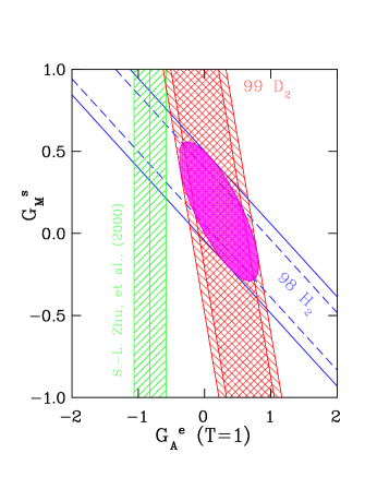
Figure 4: A result of a combined analysis of the data from the two SAMPLE measurements. The two error bands from the hydrogen experiment [4] and the deuterium experiment are indicated. The inner hatched region includes the statistical error and the outer represents the systematic uncertainty added in quadrature. The ellipse represents the allowed region for both form factors at the $1\sigma$ level. Also plotted is the estimate of the isovector axial $e-N$ form factor $G_{A}^{e}~{}(T=1)$, obtained by using the anapole form factor and radiative corrections of Zhu et al. [208].

5.2 Strange form factors of baryons in chiral models

In this section we will revisit the symmetry breaking mass effects to investigate the V-spin symmetric Coleman-Glashow sum rules [25] in the framework of the perturbative scheme, where the representation mixing coefficients can be obtained in the quantum mechanical perturbation theory, differently from the Yabu-Ando approach discussed in the previous section with the direct diagonalization.

In the perturbative method, the Hamiltonian is split up into $H=H_{0}+H_{SB}$ where $H_{0}$ is the SU(3) flavor symmetric part given by (2.41) and the symmetry breaking part is described by

$$H_{SB}=m(1-D^{8}_{88})$$ (5.20)

with $m$ the inertia parameter corresponding to $\omega$ of (3.24) in the Yabu-Ando method where the Hamiltonian has been divided into the representation independent and dependent parts.

Provided one includes the representation mixing as in the previous section, the baryon wave function is described in terms of the higher representation

$$|B\rangle=|B\rangle^{8}-C_{\bar{10}}^{B}|B\rangle^{\bar{10}}-C_{27}^{B}|B\rangle^{27}$$ (5.21)

where the representation mixing coefficients are explicitly calculated as

$$C_{\lambda}^{B}=\frac{{}_{\lambda}\langle B|H_{SB}|B\rangle_{8}}{E_{\lambda}-E_{8}}$$ (5.22)

with the eigenvalues $E_{\lambda}$ and eigenfunctions $|B\rangle^{\lambda}=\Phi_{B}^{\lambda}\otimes|{\rm intrinsic}\rangle$ of the equation $H_{0}|B\rangle^{\lambda}=E_{\lambda}|B\rangle^{\lambda}$. Here $\Phi_{B}^{\lambda}$ is the collective wavefunction discussed above and the intrinsic state degenerate to all the baryons is described by a Fock state of the quark operator and the classical meson configuration.

Using the octet wavefunctions with the higher representation mixing coefficients (5.22), the additional hyperfine structure of the magnetic moment spectrum in the quantum mechanical perturbative scheme is given by

$$\delta\mu_{B}^{i}=-2\sum_{\lambda=\bar{10},27}\frac{{}_{8}\langle B|\hat{\mu}^{i}|B\rangle_{\lambda}{}_{\lambda}\langle B|H_{SB}|B\rangle_{8}}{E_{\lambda}-E_{8}}$$ (5.23)

up to the first order of $m$, the strength of the symmetry breaking in (5.20). It is interesting here to note that one has the off-diagonal matrix elements of the magnetic moment operators $\hat{\mu}^{i}$ with higher representations $\bar{\bf 10}$ and ${\bf 27}$, differently from the diagonal matrix elements of the chiral symmetric magnetic moments in the section 3.1. This fact is presumably related to the existence of exotic states [211] belonging to $\bar{\bf 10}$ and ${\bf 27}$, which decay to the initial states in ${\bf 8}$ through the channel of the operator $D_{88}^{8}$ related to the symmetry breaking mass effects.

One can then obtain the V-spin symmetry relations in the perturbative corrections of the octet magnetic moments

$$\delta\mu_{p} = \delta\mu_{\Xi^{-}}=m{\cal I}_{2}(\frac{2}{125}{\cal M}+\frac{8}{1125}({\cal N}-2{\cal N}^{\prime}))$$

$$\delta\mu_{n} = \delta\mu_{\Sigma^{-}}=m{\cal I}_{2}(\frac{31}{750}{\cal M}-\frac{46}{1125}({\cal N}-\frac{21}{23}{\cal N}^{\prime}))$$

$$\delta\mu_{\Sigma^{+}} = \delta\mu_{\Xi^{0}}=m{\cal I}_{2}(\frac{1}{125}{\cal M}+\frac{4}{1125}({\cal N}-2{\cal N}^{\prime}))$$

$$\delta\mu_{\Lambda} = m{\cal I}_{2}(\frac{9}{500}{\cal M}+\frac{1}{125}({\cal N}-2{\cal N}^{\prime}))$$

$$\delta\mu_{\Sigma^{0}} = m{\cal I}_{2}(\frac{37}{1500}{\cal M}-\frac{7}{375}({\cal N}-\frac{17}{21}{\cal N}^{\prime}))$$ (5.24)

where the operator $\hat{\mu}^{i}_{FSB}$ is neglected due to its small contributions.

Here one notes that the above V-spin symmetric relations come from the SU(3) group theoretical fact that the matrix elements of the operators in (5.23), such as $\langle 8|D_{38}^{8}+\frac{1}{\sqrt{3}}D_{88}^{8}|\lambda\rangle\langle\lambda|D_{88}^{8}|8\rangle$, have degeneracy for the V-spin multiplets $(p$, $\Xi^{-})$, $(n$, $\Sigma^{-}$) and ($\Xi^{0}$, $\Sigma^{+}$) as in the U-spin symmetry of the section 3.1. Also as in the Yabu-Ando approach since the baryon wavefunctions in the multiquark structure of the CBM act on the magnetic moment operators with the quark and meson phase contributions in their inertia parameters, one could have the meson cloud content in the qqq$\bar{\rm q}$q multiquark Fock subspace of the chiral bag.

Now we consider the form factors of the baryon octet with internal structure in the framework of the CBM. The baryons in the CBM are definitely extended objects with internal structure characterized by the bag radius and dressed by the meson cloud. As discussed before, the $F_{2}(0)$ is interpreted as the anomalous magnetic moments of the baryon octet $\mu^{an}=\mu-Q$ whose numerical values can be easily obtained from Table 6 by subtracting the corresponding electric charges. Here one should note that the EM currents $J_{EM}^{\mu}$ obtainable from (2.6) are conserved as mentioned before and the charge density operator is a constant of motion so that the EM charge operator can be quantized in a conventional way even though the EM charge density is modified due to the derivative dependent symmetry breaking terms.

In the strange flavor sector, the strange form factors [8] at zero momentum transfer can be calculated from Eqs. (3.18) and (5.12) to yield

$$\begin{array}[]{ll}F^{(s)}_{2N}(0)=-3\mu^{(s)}_{N},&F^{(s)}_{2\Lambda}(0)=-3\mu^{(s)}_{\Lambda}-1,\\ F^{(s)}_{2\Sigma}(0)=-3\mu^{(s)}_{\Sigma}-1,&F^{(s)}_{2\Xi}(0)=-3\mu^{(s)}_{\Xi}-2.\end{array}$$ (5.25)

Note that the I-spin symmetric relation in Eq. (3.19) can be expressed in a simpler form as

$$F^{(u)}_{2B}(0)=F^{(d)}_{2,\bar{B}}(0).$$ (5.26)

Now the baryon octet strange form factors in Eq. (5.25) can be explicitly splitted into three pieces as follows

$$F_{2B}^{(s)}=F_{2B}^{(s),0}({\cal M},{\cal N},{\cal N}^{\prime})+F_{2B}^{(s),1}({\cal P},{\cal Q})+\delta F_{2B}^{(s),2}(m{\cal I}_{2}).$$ (5.27)

Table 6: The strange form factors of baryon octet

	$F^{(s),0}_{2N}$	$\delta F^{(s),1}_{2N}$	$\delta F^{(s),2}_{2N}$	$F^{(s)}_{2N}$	$F^{(s)}_{2\Lambda}$	$F^{(s)}_{2\Xi}$	$F^{(s)}_{2\Sigma}$	$F^{0}_{2}$
Fit	0.16	0.28	$-0.07$	0.37	1.37	1.22	$-0.99$	0.26
CBM	$-0.19$	$-0.12$	0.61	0.30	0.49	0.25	$-1.54$	$-0.67$
SM	$-0.13$	$-0.09$	0.20	$-0.02$	0.51	0.09	$-1.74$	$-0.67$

In the adjoint representation, one can obtain the CS and explicit current FSB contributions to the strange form factors

$$F_{2N}^{(s),0} = \frac{7}{20}{\cal M}-\frac{1}{15}({\cal N}+\frac{1}{2}{\cal N}^{\prime})$$

$$F_{2\Lambda}^{(s),0} = \frac{9}{20}{\cal M}+\frac{1}{5}({\cal N}+\frac{1}{2}{\cal N}^{\prime})-1$$

$$F_{2\Xi}^{(s),0} = \frac{3}{5}{\cal M}+\frac{4}{15}({\cal N}+\frac{1}{2}{\cal N}^{\prime})-2$$

$$F_{2\Sigma}^{(s),0} = \frac{11}{20}{\cal M}-\frac{1}{5}({\cal N}+\frac{1}{2}{\cal N}^{\prime})-1$$ (5.28)

and

$$\begin{array}[]{ll}F_{2N}^{(s),1}=-\frac{1}{15}{\cal P}-\frac{1}{30}{\cal Q},&F_{2\Lambda}^{(s),1}=\frac{1}{5}{\cal P}+\frac{1}{10}{\cal Q}\\ F_{2\Xi}^{(s),1}=\frac{1}{3}{\cal P}+\frac{1}{15}{\cal Q},&F_{2\Sigma}^{(s),1}=-\frac{11}{45}{\cal P}-\frac{1}{18}{\cal Q}.\\ \end{array}$$ (5.29)

Treated in the quantum mechanical perturbative scheme of the previous section, the representation mixing coefficients from the multiquark structure can be explicitly given as

$$\delta F_{2N}^{(s),2} = m{\cal I}_{2}(-\frac{43}{750}{\cal M}+\frac{38}{1125}{\cal N}-\frac{26}{1125}{\cal N}^{\prime})$$

$$\delta F_{2\Lambda}^{(s),2} = m{\cal I}_{2}(-\frac{9}{250}{\cal M}-\frac{2}{125}{\cal N}+\frac{4}{125}{\cal N}^{\prime})$$

$$\delta F_{2\Xi}^{(s),2} = m{\cal I}_{2}(-\frac{3}{125}{\cal M}-\frac{4}{375}{\cal N}+\frac{8}{375}{\cal N}^{\prime})$$

$$\delta F_{2\Sigma}^{(s),2} = m{\cal I}_{2}(-\frac{37}{750}{\cal M}+\frac{14}{375}{\cal N}-\frac{34}{1125}{\cal N}^{\prime}).$$ (5.30)

Next using the flavor singlet vector currents $J_{V}^{\mu 0}$, which can be constructed by replacing $\hat{Q}_{a}$ by $1$ in (2.6), instead of the EM currents in the matrix element (5.4) we can also obtain the flavor singlet form factors [8, 35, 6]

$$F_{2}^{0}=\frac{1}{2}{\cal M}-1$$ (5.31)

which are degenerate with all the baryon octet even in the multiquark structure regardless of whether one uses the Yabu-Ando or perturbative methods.

In Table 6 one can acquire the numerical values for the strange form factors and flavor singlet form factors.

6 Unification of chiral bag model with other models

6.1 Connection to naive nonrelativistic quark model

Until now we have considered the static properties such as the magnetic moments and form factors of the baryon octet in the CBM which unifies the MIT bag and Skyrmion models with the bag radius parameter. In this section we will relate the CBM with the naive NRQM by investigating the model-independent sum rules in the magnetic moments, which have been already derived in the CBM in the previous sections for the baryon octet and decuplet to have a clue for the unification of the naive NRQM into the CBM.

In the naive NRQM, the wave function of a baryon consists of several degrees of freedom [212]

$$\psi({\rm baryon})=\psi({\rm space})\psi({\rm spin})\psi({\rm flavor})\psi({\rm color})$$ (6.1)

where the spatial wave function is symmetric in the ground state, and the spin state can either be completely symmetric ($J=\frac{3}{2}$) or of mixed symmetry ($J=\frac{1}{2}$), and there are $3^{3}$ flavor combinations which can be reshuffled into irreducible representations of SU(3), and the color wave function is antisymmetric and degenerate to all the baryons since every naturally occurring baryon is a color singlet, and the full baryon wave function is antisymmetric under the interchange of any two quarks.

The baryon octet wave function is then constructed by the nontrivial spin/flavor wave function of the form

$$\psi({\rm baryon~{}octet})=\frac{\sqrt{2}}{3}(\psi_{12}({\rm spin})\psi_{12}({\rm flavor})+{\rm two~{}other~{}terms})$$ (6.2)

where $\psi_{ij}({\rm spin})$ and $\psi_{ij}({\rm flavor})$ are the states with mixed symmetry such that their product is completely symmetric in quarks $i$ and $j$. Since each quark has the intrinsic spin in itself the baryon magnetic moments in the naive NRQM are obtained by linearly adding the magnetic angular momentum quantum number of the wave function. The baryon octet magnetic moments and the $\Lambda\Sigma^{0}$ transition matrix element can then be constructed in terms of linear vector sum of the three constituent quark magnetic moments $\mu_{q}$ (q=u,d,s) [213]

$$\mu_{p} = \frac{1}{3}(4\mu_{u}-\mu_{d}),~{}~{}~{}~{}\mu_{n}=\frac{1}{3}(-\mu_{u}+4\mu_{d})$$

$$\mu_{\Sigma^{-}} = \frac{1}{3}(4\mu_{d}-\mu_{s}),~{}~{}~{}~{}\mu_{\Sigma^{0}}=\frac{1}{3}(2\mu_{u}+2\mu_{d}-\mu_{s}),$$

$$\mu_{\Sigma^{+}} = \frac{1}{3}(4\mu_{u}-\mu_{s}),~{}~{}~{}~{}\mu_{\Xi^{-}}=\frac{1}{3}(-\mu_{d}+4\mu_{s}),$$

$$\mu_{\Xi^{0}} = \frac{1}{3}(-\mu_{u}+4\mu_{s}),~{}~{}~{}~{}\mu_{\Lambda}=\mu_{s}$$

$$\frac{1}{\sqrt{3}}\mu_{\Lambda\Sigma^{0}} = \frac{1}{3}(-4\mu_{u}-\mu_{d}),$$ (6.3)

where $\mu_{q}=Q_{q}(m_{N}/m_{q})$ in unit of nuclear magnetons (=$e\hbar/2m_{N}c$) with $m_{q}$ the q-flavor quark mass and $m_{N}$ the nucleon mass. Here one notes that due to $\mu_{u}/\mu_{d}=-2$ one has the ratio $\mu_{n}/\mu_{p}=-\frac{2}{3}$ comparable to the experimental value $-0.69$ and the CBM prediction $-\frac{3}{4}$ in the leading order of $N_{c}$.

Since the d- and s-flavor charges are degenerate in the SU(3) EM charge operator $\hat{Q}_{EM}$, the baryon magnetic moments in the SU(3) flavor symmetric limit with the chiral symmetry breaking masses $m_{u}=m_{d}=m_{s}$ satisfy the U-spin symmetric Coleman-Glashow sum rules in the naive NRQM, the analogy of the U-spin symmetry relations (3.3) in the CBM

$$\mu_{\Sigma^{+}} = \mu_{p}=\frac{m_{N}}{m_{u}}$$

$$\mu_{\Xi^{0}} = \mu_{n}=-\frac{2}{3}\frac{m_{N}}{m_{u}}$$

$$\mu_{\Xi^{-}} = \mu_{\Sigma^{-}}=-\frac{1}{3}\frac{m_{N}}{m_{u}}$$

$$\mu_{\Sigma^{0}} = -\mu_{\Lambda}=\frac{1}{3}\frac{m_{N}}{m_{u}}$$ (6.4)

and the other Coleman-Glashow sum rule (3.5) for the summation of the magnetic moments over all the octet baryons. The naive NRQM also predicts the other sum rules (3.7) and the relations of the hyperon and transition magnetic moments in terms of the nucleon magnetic moments (3.8) in the CBM.

Using the projection operators (3.14) one can easily see that the nucleon magnetic moments in the u-flavor channel of the naive NRQM are given by $\mu_{p}^{(u)}=\frac{4}{3}Q_{u}(m_{N}/m_{u})$ and $\mu_{n}^{(u)}=-\frac{1}{3}Q_{u}(m_{N}/m_{u})$, and the d-flavor components of nucleon magnetic moments are given by (3.20) as in the CBM, but $\mu_{N}^{(s)}=0$ due to the absence of the strange quarks in the nucleon of the naive NRQM. In general, one can easily see that the SU(3) flavor components of hyperon magnetic moments also satisfy the identities (3.20) in the naive NRQM.

In the more general SU(3) flavor symmetry breaking case with $m_{u}=m_{d}\neq\mu_{s}$ one can easily see that the baryon octet magnetic moments fulfill the Coleman-Glashow sum rule (3.4), since $\mu_{\Sigma^{+}}+\mu_{\Sigma^{-}}$ is independent of the third component of the isospin, and the last model-independent relation in (3.8) and the identities in (3.20) hold since they are the relations derived in the same strangeness sector.

Together with the above model-independent Coleman-Glashow sum rules shared by two models, the CBM predictions propose the unification of the naive NRQM and the CBM which has the meson cloud, around the quarks of the naive NRQM, located both in the quark and meson phases. In other words, the CBM can be phenomenologically proposed as an effective NRQM in the adjoint representation and model-independent relations and Cheshire cat properties are shown to support the effective NRQM conjecture with meson cloud.

In Table 2 the SU(2) CBM predictions [28] are explicitly listed to be compared with the naive NRQM and SU(3) CBM so that the pure kaon contributions to the baryon magnetic moments can be explicitly calculated with respect to the naive NRQM.

Next starting with the symmetric spin configuration in the ground state with symmetric $\psi({\rm space})$ one can have the spin-$\frac{3}{2}$ baryon decuplet wave function in the naive NRQM with the symmetric flavor state to yield

$$\psi({\rm baryon~{}decuplet})=\psi_{s}({\rm spin})\psi_{s}({\rm flavor}).$$ (6.5)

In the naive NRQM the baryon magnetic moments are then obtained as the linear sum of the three constituent quark magnetic moments, similarly to (6.3)

$$\mu_{\Delta^{-}} = 3\mu_{d},~{}~{}~{}~{}\mu_{\Delta^{0}}=\mu_{u}+2\mu_{d}$$

$$\mu_{\Delta^{+}} = 2\mu_{d}+\mu_{d},~{}~{}~{}~{}\mu_{\Delta^{++}}=3\mu_{u},$$

$$\mu_{\Sigma^{*-}} = 2\mu_{u}+\mu_{s},~{}~{}~{}~{}\mu_{\Sigma^{*0}}=\mu_{u}+\mu_{d}+\mu_{s},$$

$$\mu_{\Sigma^{*+}} = 2\mu_{u}+\mu_{s},~{}~{}~{}~{}\mu_{\Xi^{*-}}=\mu_{d}+2\mu_{s}$$

$$\mu_{\Xi^{*0}} = \mu_{u}+2\mu_{s},~{}~{}~{}~{}\mu_{\Omega^{-}}=3\mu_{s}.$$ (6.6)

In the SU(3) flavor symmetric limit with the chiral symmetry breaking masses $m_{u}=m_{d}=m_{s}$, the decuplet baryons with the EM charge $Q_{EM}$ are described by [189]

$$\mu_{B}=Q_{EM}\frac{m_{N}}{m_{u}}$$ (6.7)

and satisfy the U-spin symmetry relations (4.4) and (4.7).

On the other hand the $\Delta$ magnetic moments in the u- and s-flavor channels are given by

$$\mu_{\Delta}^{(u)}=(Q+1)\frac{2}{3}\frac{m_{N}}{m_{u}},~{}~{}~{}~{}\mu_{\Delta}^{(s)}=0,$$ (6.8)

and in general all the baryon decuplet magnetic moments fulfill the model-independent relations (3.20) in the u- and d-flavor components and the I-spin symmetry in the s-flavor channel where the isomultiplets have the degenerate strangeness number.

Finally one should note that the other sum rules (4.5) and (4.6) and the identities in (3.20) hold even in the SU(3) flavor symmetry breaking case ($m_{u}=m_{d}\neq m_{s}$) since they are the relations derived in the same strangeness sector.

The above model-independent sum rules in the baryon decuplet satisfied by the naive NRQM and the CBM support the effective NRQM conjecture as in the baryon octet. The effective NRQM conjecture discussed in the baryon octet and decuplet support the possibility of the unification of the CBM with the naive NRQM while the Cheshire catness suggests another clue to the unification of the CBM with the Skyrmion model. In the next section we will proceed to consider the other plausible unification of the CBM with the NJL model, chiral perturbation theory, CK model and chiral quark soliton model.

6.2 Connection to other models

So far the chiral soliton model such as the Skyrmion model have been constructed mainly on the basis of the low-energy meson phenomenology since the effective meson Lagrangian underlying QCD is not known. There has been some progress in deriving effective meson Lagrangian either directly from QCD [214] or from the quark flavor dynamics [215] of the NJL model [216]. Especially it has been claimed that the Skyrmion model can be derived [217, 218] from the NJL model in the limit of large vector and axial-vector meson masses. Consequently one may claim that there can be plausibility in the unification of the CBM with the NJL model.

Next in the strong chiral symmetry breaking limit the Yabu-Ando approach to the Skyrmion model has suggested [82] the mass formula similar to the one derived in the bound state scheme in CK model so that one may conclude that the perturbation and bound state schemes are two extreme limits of the Yabu-Ando approach. Similarly, in the large limit of the symmetry breaking strength $\omega$ of (3.24), the CBM results are comparable to those of Refs. [219, 220] estimated in the bound state scheme of CK model.

Finally, in the chiral quark soliton model [221], the baryon decuplet magnetic moments satisfy the model independent sum rules (4.4) and (4.7) as in the naive NRQM. Moreover one can easily see that the CBM shares with the naive NRQM and chiral quark soliton model the following sum rules

$$-4\mu_{\Delta^{++}}+6\mu_{\Delta^{+}}+3\mu_{\Sigma^{*+}}-6\mu_{\Sigma^{*0}}+\mu_{\Omega^{-}} = 0$$ (6.9)

$$-2\mu_{\Delta^{++}}+3\mu_{\Delta^{+}}+2\mu_{\Sigma^{*+}}-4\mu_{\Sigma^{*0}}+\mu_{\Xi^{*-}} = 0$$ (6.10)

$$-\mu_{\Delta^{++}}+2\mu_{\Delta^{+}}-2\mu_{\Sigma^{*0}}+\mu_{\Xi^{*0}} = 0$$ (6.11)

$$\mu_{\Delta^{++}}-2\mu_{\Delta^{+}}+\mu_{\Delta^{0}} = 0$$ (6.12)

and

$$\mu_{\Delta^{0}}-\mu_{\Sigma^{*-}}=\mu_{\Sigma^{*+}}-\mu_{\Xi^{*0}}=\frac{1}{2}(\mu_{\Delta^{+}}-\mu_{\Xi^{*-}})=\frac{1}{3}(\mu_{\Delta^{++}}-\mu_{\Omega^{-}}).$$ (6.13)

These sum rules also suggest the possibility of unification of the CBM with the naive NRQM and chiral quark soliton model.

7 Improved Dirac quantization of Skyrmion model

7.1 Modified mass spectrum in SU(2) Skyrmion

In this section, we will apply the Batalin-Fradkin-Tyutin (BFT) method to the Skyrmion to obtain the modified mass spectrum of the baryons by including the Weyl ordering correction. We will next canonically quantize the SU(2) Skyrme model by using the Dirac quantization method, which will be shown to be consistent with the BFT one after the adjustable parameters are introduced to define the generalized momenta without any loss of generality [94].

Now we start with the SU(2) Skyrmion Lagrangian of the form

$$L_{SM}=\int{\rm d}r^{3}\left[-\frac{1}{4}f_{\pi}^{2}{\rm tr}(l_{\mu}l^{\mu})+\frac{1}{32e^{2}}{\rm tr}[l_{\mu},l_{\nu}]^{2}\right]$$ (7.1)

where $l_{\mu}=U^{\dagger}\partial_{\mu}U$ and $U$ is an SU(2) matrix satisfying the boundary condition $\lim_{r\rightarrow\infty}U=I$ so that the pion field vanishes as $r$ goes to infinity.

On the other hand, in the Skyrmion model, since the hedgehog ansatz has maximal or spherical symmetry, it is easily seen that spin plus isospin equals zero, so that isospin transformations and spatial rotations are related to each other. Furthermore spin and isospin states can be treated by collective coordinates $a^{\mu}=(a^{0},\vec{a})$ $(\mu=0,1,2,3)$ corresponding to the spin and isospin rotations

$$A(t)=a^{0}+i\vec{a}\cdot\vec{\tau},$$ (7.2)

which is the time dependent collective variable defined on the SU(2)_F group manifold and is related with the zero modes associated with the collective rotation (2.31) in the SU(3) CBM. With the hedgehog ansatz described in section 1.4 and the collective rotation $A(t)\in$ SU(2), the chiral field can be given by $U(\vec{x},t)=A(t)U_{0}(\vec{x})A^{\dagger}(t)=e^{i\tau_{a}R_{ab}\hat{x}_{b}f(r)}$ where $R_{ab}=\frac{1}{2}{\rm tr}(\tau_{a}A\tau_{b}A^{\dagger})$ and the Skyrmion Lagrangian can be written as

$$L_{SM}=-M_{0}+2{\cal I}_{10}\dot{a}^{\mu}\dot{a}^{\mu}$$ (7.3)

where $M_{0}$ and ${\cal I}_{10}$ are the static mass and the moment of inertia given as

$$M_{0} = \frac{2\pi f_{\pi}}{e}\int_{0}^{\infty}{\rm d}z~{}z^{2}\left(\left(\frac{d\theta}{dz}\right)^{2}+\left(2+2\left(\frac{d\theta}{dz}\right)^{2}+\frac{\sin^{2}\theta}{z^{2}}\right)\frac{\sin^{2}\theta}{z^{2}}\right)$$ (7.4)

$${\cal I}_{10} = \frac{8\pi}{3e^{3}f_{\pi}}\int_{0}^{\infty}{\rm d}z~{}z^{2}\sin^{2}\theta\left(1+\left(\frac{d\theta}{dz}\right)^{2}+\frac{\sin^{2}\theta}{z^{2}}\right)$$ (7.5)

with the dimensionless quantity $z=ef_{\pi}r$.

Introducing the canonical momenta $\pi^{\mu}=4{\cal I}_{10}\dot{a}^{\mu}$ conjugate to the collective coordinates $a^{\mu}$ one can then obtain the canonical Hamiltonian

$$H=M_{0}+\frac{1}{8{\cal I}_{10}}\pi^{\mu}\pi^{\mu}.$$ (7.6)

and the spin and isospin operators

$$J^{i} = \frac{1}{2}(a^{0}\pi^{i}-a^{i}\pi^{0}-\epsilon_{ijk}a^{j}\pi^{k}),$$

$$I^{i} = \frac{1}{2}(a^{i}\pi^{0}-a^{0}\pi^{i}-\epsilon_{ijk}a^{j}\pi^{k}).$$ (7.7)

On the other hand our system has the second class constraints

$$\Omega_{1}=a^{\mu}a^{\mu}-1\approx 0,~{}~{}~{}\Omega_{2}=a^{\mu}\pi^{\mu}\approx 0,$$ (7.8)

to yield the Poisson algebra with $\epsilon^{12}=-\epsilon^{21}=1$

$$\Delta_{kk^{\prime}}=\{\Omega_{k},\Omega_{k^{\prime}}\}=2\epsilon^{kk^{\prime}}a^{\mu}a^{\mu}.$$ (7.9)

We now recapitulate the construction of the first class SU(2) Hamiltonian. Following the BFT formalism [89, 94, 222] we introduce two auxiliary fields $(\theta,\pi_{\theta})$ with the Poisson brackets

$$\{\theta,\pi_{\theta}\}=1.$$ (7.10)

One can then obtain the first class constraints

$$\tilde{\Omega}_{1}=\Omega_{1}+2\theta,~{}~{}~{}\tilde{\Omega}_{2}=\Omega_{2}-a^{\mu}a^{\mu}\pi_{\theta},$$ (7.11)

satisfying the first class constraint Lie algebra $\{\tilde{\Omega}_{i},\tilde{\Omega}_{j}\}=0$. Demanding that they are strongly involutive in the extended phase space, i.e., $\{\tilde{\Omega}_{i},\tilde{{\cal F}}\}=0$, one can construct the first class BFT physical fields $\tilde{{\cal F}}=(\tilde{a}^{\mu},\tilde{\pi}^{\mu})$ corresponding to the original fields ${\cal F}=(a^{\mu},\pi^{\mu})$, as a power series of the auxiliary fields $(\theta,\pi_{\theta})$

$$\tilde{a}^{\mu} = a^{\mu}\left(\frac{a^{\mu}a^{\mu}+2\theta}{a^{\mu}a^{\mu}}\right)^{1/2}$$

$$\tilde{\pi}^{\mu} = (\pi^{\mu}-a^{\mu}\pi_{\theta})\left(\frac{a^{\mu}a^{\mu}}{a^{\mu}a^{\mu}+2\theta}\right)^{1/2}.$$ (7.12)

As discussed in Ref. [92], any functional ${\cal K}(\tilde{{\cal F}})$ of the first class fields $\tilde{{\cal F}}$ is also first class, namely, $\tilde{{\cal K}}({\cal F};\Phi)={\cal K}(\tilde{{\cal F}})$. Using the property, we construct a first-class Hamiltonian in terms of the above BFT physical variables. The result is

$$\tilde{H}=M_{0}+\frac{1}{8{\cal I}_{10}}\tilde{\pi}^{\mu}\tilde{\pi}^{\mu}.$$ (7.13)

We then directly rewrite this Hamiltonian in terms of the original as well as auxiliary fields [95]

$$\tilde{H}=M_{0}+\frac{1}{8{\cal I}_{10}}(\pi^{\mu}-a^{\mu}\pi_{\theta})(\pi^{\mu}-a^{\mu}\pi_{\theta})\frac{a^{\nu}a^{\nu}}{a^{\nu}a^{\nu}+2\theta},$$ (7.14)

which is also strongly involutive with the first class constraints $\{\tilde{\Omega}_{i},\tilde{H}\}=0$. However, with the first class Hamiltonian (7.14), one cannot naturally generate the first class Gauss’ law constraint from the time evolution of the primary constraint $\tilde{\Omega}_{1}$. Now, by introducing an additional term proportional to the first class constraints $\tilde{\Omega}_{2}$ into $\tilde{H}$, we obtain an equivalent first class Hamiltonian

$$\tilde{H}^{\prime}=\tilde{H}+\frac{1}{4{\cal I}_{10}}\pi_{\theta}\tilde{\Omega}_{2},$$ (7.15)

which naturally generates the Gauss’ law constraint

$$\{\tilde{\Omega}_{1},\tilde{H}^{\prime}\}=\frac{1}{2{\cal I}_{10}}\tilde{\Omega}_{2},~{}~{}~{}\{\tilde{\Omega}_{2},\tilde{H}^{\prime}\}=0.$$ (7.16)

Here one notes that $\tilde{H}$ and $\tilde{H}^{\prime}$ act on physical states in the same way since such states are annihilated by the first class constraints.

Table 7: The static properties of baryons in the standard and Weyl ordering corrected (WOC) Skyrmions compared with experimental data. The quantities used as input parameters are indicated by $*$.

Quantity	Standard	WOC	Experiment
$M_{N}$	939 MeV∗	939 MeV∗	939 MeV
$M_{\Delta}$	1232 MeV∗	1232 MeV∗	1232 MeV
$f_{\pi}$	64.5 MeV	63.2 MeV	93.0 MeV
e	5.44	5.48	$-$
$\langle r^{2}\rangle^{1/2}_{M,I=0}$	0.92 fm	0.94 fm	0.81 fm
$\langle r^{2}\rangle^{1/2}_{M,I=1}$	$\infty$	$\infty$	0.80 fm
$\langle r^{2}\rangle^{1/2}_{I=0}$	0.59 fm	0.60 fm	0.72 fm
$\langle r^{2}\rangle^{1/2}_{I=1}$	$\infty$	$\infty$	0.88 fm
$\mu_{p}$	1.87	1.89	2.79
$\mu_{n}$	$-1.31$	$-1.32$	$-1.91$
$\mu_{\Delta^{++}}$	3.72	3.75	4.7$-$6.7
$\mu_{N\Delta}$	2.27	2.27	3.29
$\mu_{p}-\mu_{n}$	3.18	3.21	4.70

Using the first class constraints in this Hamiltonian (7.15), one can obtain the Hamiltonian of the form

$$\tilde{H}^{\prime}=M_{0}+\frac{1}{8{\cal I}_{10}}(a^{\mu}a^{\mu}\pi^{\nu}\pi^{\nu}-a^{\mu}\pi^{\mu}a^{\nu}\pi^{\nu}).$$ (7.17)

Following the symmetrization procedure, the first class Hamiltonian yields the slightly modified energy spectrum with the Weyl ordering correction [223, 94, 222, 95]

$$\langle\tilde{H}^{\prime}\rangle=M_{0}+\frac{1}{2{\cal I}_{10}}\left[I(I+1)+\frac{1}{4}\right]$$ (7.18)

where $I$ is the isospin quantum number of baryons.

Next, using the Weyl ordering corrected energy spectrum (7.18), we easily obtain the hyperfine structure of the nucleon and delta hyperon masses to yield the static mass and the moment of inertia

$$M_{0}=\frac{1}{3}(4M_{N}-M_{\Delta}),~{}~{}~{}{\cal I}_{10}=\frac{3}{2}(M_{\Delta}-M_{N})^{-1}.$$ (7.19)

Substituting the experimental values $M_{N}=939$ MeV and $N_{\Delta}=1232$ MeV into Eq. (7.19) and using the expressions (7.5), one can predict the pion decay constant $f_{\pi}$ and the Skyrmion parameter $e$ as follows

$$f_{\pi}=63.2~{}{\rm MeV},~{}~{}~{}e=5.48.$$

With these fixed values of $f_{\pi}$ and $e$, one can then proceed to yield the predictions for the other static properties of the baryons. The isoscalar and isovector mean square (magnetic) charge radii and the baryon and transition magnetic moments are contained in Table 7, together with the experimental data and the standard Skyrmion predictions [64, 66, 224]. It is remarkable that the effects of Weyl ordering correction in the baryon energy spectrum are propagated through the model parameters $f_{\pi}$ and $e$ to modify the predictions of the baryon static properties.

Moreover, one can show that, by fixing a free adjustable parameter $c$ introduced to define generalized momenta, the baryon energy eigenvalues obtained by the standard Dirac method are consistent with the above BFT result. To be more specific, we can obtain the modified quantum energy spectrum of the baryons [94]

$$\langle H_{N}\rangle=M_{0}+\frac{1}{8{\cal I}_{10}}[l(l+2)+\frac{9}{4}-c^{2}]$$ (7.20)

which is consistent with the BFT result (7.18) if the adjustable parameter $c$ is fixed with the values $c=\pm\frac{\sqrt{5}}{2}$. Here one notes that these values for the parameter $c$ relate the Dirac bracket scheme with the BFT one to yield the desired quantization in the SU(2) Skyrmion model so that one can achieve the unification of these two different formalisms. (For details see Ref. [94].)

On the other hand, we can obtain the BRST invariant Lagrangian in the framework of the BFV formalism [226, 227, 228] which is applicable to theories with the first class constraints by introducing two canonical sets of ghosts and anti-ghosts together with auxiliary fields. Following the procedure in Appendix C.1, one can arrive at the BRST invariant Lagrangian [95]

$$L_{eff} = -M_{0}+\frac{2{\cal I}_{10}}{1-2\theta}\dot{a}^{\mu}\dot{a}^{\mu}-\frac{2{\cal I}_{10}}{(1-2\theta)^{2}}\dot{\theta}^{2}-2{\cal I}_{10}(1-2\theta)^{2}(B+2\bar{{\cal C}}{\cal C})^{2}$$ (7.21)

$$-\frac{\dot{\theta}\dot{B}}{1-2\theta}+\dot{\bar{{\cal C}}}\dot{{\cal C}},$$

which is invariant under the BRST transformation

$$\delta_{B}a^{\mu} = \lambda a^{\mu}{\cal C},~{}~{}~{}\delta_{B}\theta=-\lambda(1-2\theta){\cal C},$$

$$\delta_{B}\bar{{\cal C}} = -\lambda B,~{}~{}~{}\delta_{B}{\cal C}=\delta_{B}B=0.$$ (7.22)

Here ${\cal C}$ ($\bar{{\cal C}}$) and $B$ are the (anti-)ghosts and the corresponding auxiliary fields. (For details see Appendix C.1.)

7.2 Phenomenology in SU(3) Skyrmion

Now let us consider the hyperfine splittings for the SU(3) Skyrmion [78, 229, 211] which has been studied in two main schemes as discussed in the previous chapters. Firstly, the SU(3) cranking method exploits rigid rotation of the Skyrmion in the collective space of SU(3) Euler angles with full diagonalization of the flavor symmetry breaking (FSB) terms [25, 37, 38]. Especially, Yabu and Ando [82] proposed the exact diagonalization of the symmetry breaking terms by introducing higher irreducible representation mixing in the baryon wave function, which was later interpreted in terms of the multiquark structure [83, 84] in the baryon wave function. Secondly, Callan and Klebanov [79] suggested an interpretation of baryons containing a heavy quark as bound states of solitons of the pion chiral Lagrangian with mesons. In their formalism, the fluctuations in the strangeness direction are treated differently from those in the isospin directions [79, 80].

In order to generalize the standard flavor symmetric (FS) SU(3) Skyrmion rigid rotator approach [230, 231] to the SU(3) Skyrmion case with the pion mass and FSB terms, we will now investigate the chiral breaking pion mass and FSB effects on $c$ the ratio of the strange-light to light-light interaction strengths and $\bar{c}$ that of the strange-strange to light-light.

Now we start with the SU(3) Skyrmion Lagrangian of the form

$${\cal L} = -\frac{1}{4}f_{\pi}^{2}{\rm tr}(l_{\mu}l^{\mu})+\frac{1}{32e^{2}}{\rm tr}[l_{\mu},l_{\nu}]^{2}+{\cal L}_{WZW}$$

$$+\frac{1}{4}f_{\pi}^{2}{\rm tr}M(U+U^{{\dagger}}-2)+{\cal L}_{FSB},$$

$${\cal L}_{FSB} = \frac{1}{6}(f_{K}^{2}m_{K}^{2}-f_{\pi}^{2}m_{\pi}^{2}){\rm tr}((1-\sqrt{3}\lambda_{8})(U+U^{{\dagger}}-2))$$ (7.23)

$$-\frac{1}{12}(f_{K}^{2}-f_{\pi}^{2}){\rm tr}((1-\sqrt{3}\lambda_{8})(Ul_{\mu}l^{\mu}+l_{\mu}l^{\mu}U^{{\dagger}})),$$

where $f_{\pi}$ ($f_{K}$) and $e$ are the pion (kaon) decay constants and the dimensionless Skyrme parameter as before. Here $l_{\mu}=U^{{\dagger}}\partial_{\mu}U$ with an SU(3) matrix $U$ and $M$ is proportional to the quark mass matrix given by

$$M={\rm diag}~{}(m_{\pi}^{2},~{}m_{\pi}^{2},~{}2m_{K}^{2}-m_{\pi}^{2}),$$

where $m_{\pi}=138$ MeV and $m_{K}=495$ MeV. Note that ${\cal L}_{FSB}$ is the FSB correction term due to the relations $m_{\pi}\neq m_{K}$ and $f_{\pi}\neq f_{K}$ [232, 25] and the Wess-Zumino-Witten (WZW) term [78] is described by the action

$$\Gamma_{WZW}=-\frac{iN_{c}}{240\pi^{2}}\int_{{\sf M}}{\rm d}^{5}r\epsilon^{\mu\nu\alpha\beta\gamma}{\rm tr}(l_{\mu}l_{\nu}l_{\alpha}l_{\beta}l_{\gamma}),$$ (7.24)

where $N_{c}$ is the number of colors and the integral is done on the five-dimensional manifold ${\sf M}=V\times S^{1}\times I$ with the three-space volume $V$, the compactified time $S^{1}$ and the unit interval $I$ needed for a local form of WZW term. Here note that we have used the three-space volume $V$ instead of $\bar{V}$ of the CBM case.

Using Eq. (C.20) in Appendix C.2 and following the Klebanov and Westerberg’s quantization scheme [230] for the strangeness flavor direction in the BFT formalism, one can obtain the Hamiltonian of the form

$$H = M_{0}+\frac{1}{2}\Gamma_{0}m_{\pi}^{2}+\frac{1}{2{\cal I}_{10}}(\vec{I}^{2}+\frac{1}{4})+\frac{N_{c}}{8{\cal I}_{20}^{\prime}}(\mu_{K}-1)a^{{\dagger}}a$$ (7.25)

$$+\left[\frac{1}{2{\cal I}_{10}}-\frac{1}{4{\cal I}_{20}^{\prime}\mu_{K}}\left(1+\frac{\Gamma_{2}}{{\cal I}_{10}}\right)(\mu_{K}-1)\right]a^{{\dagger}}\vec{I}\cdot\vec{\tau}a$$

$$+\left[\frac{1}{8{\cal I}_{10}}-\frac{1}{8{\cal I}_{20}^{\prime}\mu_{K}^{2}}\left(1+\frac{\Gamma_{2}}{{\cal I}_{10}}\mu_{K}\right.\right.$$

$$\left.\left.-\frac{\Gamma_{2}^{2}+2{\cal I}_{10}(\Gamma_{1}-\Gamma_{2})}{4{\cal I}_{10}{\cal I}_{20}^{\prime}}(\mu_{K}-1)\right)(\mu_{K}-1)\right](a^{{\dagger}}a)^{2},$$

where

$$\mu_{K}=\left(1+\frac{\chi^{2}m_{K}^{2}-m_{\pi}^{2}+\Gamma_{3}/\Gamma_{0}}{m_{0}^{2}}\right)^{1/2},~{}~{}~{}m_{0}=\frac{N_{c}}{4(\Gamma_{0}{\cal I}_{20}^{\prime})^{1/2}}$$

and $a^{{\dagger}}$ is creation operator for constituent strange quarks and we have ignored the irrelevant creation operator $b^{{\dagger}}$ for strange antiquarks [230]. Then, introducing the angular momentum of the strange quarks $\vec{J}_{s}=\frac{1}{2}a^{{\dagger}}\vec{\tau}a$, one can rewrite the Hamiltonian (7.25) as

$$H=M_{0}+\frac{1}{2}\Gamma_{0}m_{\pi}^{2}+\omega a^{{\dagger}}a+\frac{1}{2{\cal I}_{10}}\left(\vec{I}^{2}+2c\vec{I}\cdot\vec{J}_{s}+\bar{c}\vec{J}_{s}^{2}+\frac{1}{4}\right)$$ (7.26)

where

$$\omega = \frac{N_{c}}{8{\cal I}_{20}^{\prime}}(\mu_{K}-1),$$

$$c = 1-\frac{{\cal I}_{10}}{2{\cal I}_{20}^{\prime}\mu_{K}}\left(1+\frac{\Gamma_{2}}{{\cal I}_{10}}\right)(\mu_{K}-1),$$

$$\bar{c} = 1-\frac{{\cal I}_{10}}{{\cal I}_{20}^{\prime}\mu_{K}^{2}}\left(1+\frac{\Gamma_{2}}{{\cal I}_{10}}\mu_{K}-\frac{\Gamma_{2}^{2}+2{\cal I}_{10}(\Gamma_{1}-\Gamma_{2})}{4{\cal I}_{10}{\cal I}_{20}^{\prime}}(\mu_{K}-1)\right)(\mu_{K}-1).$$

Here note that the FSB effects are included in $c$ and $\bar{c}$, through $\Gamma_{1}$, $\Gamma_{2}$, ${\cal I}_{20}^{\prime}$ and $\chi$ and $\Gamma_{3}$ in $\mu_{K}$.

Table 8: The values of $c$ and $\bar{c}$ in the massless pion and massive pion rigid rotator approaches to the SU(3) Skyrmions compared with experimental data. For the rigid rotator approaches, both the predictions in the flavor symmetric (FS) case and flavor symmetry breaking (FSB) one are listed.

Source	$c$	$\bar{c}$
Rigid rotator, massless and FS	0.92	0.86
Rigid rotator, massless and FSB	0.82	0.69
Rigid rotator, massive and FS	0.79	0.66
Rigid rotator, massive and FSB	0.67	0.56
Experiment	0.67	0.27

The Hamiltonian (7.26) then yields the structure of the hyperfine splittings as follows

$$\delta M = \frac{1}{2{\cal I}_{10}}\left[cJ(J+1)+(1-c)\left(I(I+1)-\frac{Y^{2}-1}{4}\right)\right.$$ (7.27)

$$\left.+(1+\bar{c}-2c)\frac{Y^{2}-1}{4}+\frac{1}{4}(1+\bar{c}-c)\right],$$

where $\vec{J}=\vec{I}+\vec{J}_{s}$ is the total angular momentum of the quarks, and $c$ and $\bar{c}$ are the modified quantities due to the existence of the FSB effect as shown above.

Now using the experimental values of the pion and kaon decay constants $f_{\pi}=93$ MeV and $f_{K}=114$ MeV, we fix the value of the Skyrmion parameter $e$ to fit the experimental data of $c_{exp}=0.67$ to yield the predictions for the values of $c$ and $\bar{c}$

$$c=0.67,~{}~{}~{}\bar{c}=0.56$$ (7.28)

which are contained in Table 8, together with the experimental data and the SU(3) rigid rotator predictions without pion mass. For the massless and massive rigid rotator approaches we have used the above values for the decay constants $f_{\pi}$ and $f_{K}$ to obtain both the predictions in the FS and FSB cases. As a result, we have explicitly shown that the more realistic physics considerations via the pion mass and the FSB terms improve both the $c$ and $\bar{c}$ values, as shown in Table 8 [97].

7.3 Berry phase and Casimir energy in SU(3) Skyrmion

Now we investigate the relations between the Hamiltonian (7.26) and the Berry phases [233]. In the Berry phase approach to the SU(3) Skyrmion, the Hamiltonian takes the simple form [39]

$$H^{*}=\epsilon_{K}+\frac{1}{8{\cal I}_{1}}(\vec{R}^{2}-2g_{K}\vec{R}\cdot\vec{T}_{K}+g_{K}^{2}\vec{T}_{K}^{2})$$ (7.29)

where $\epsilon_{K}$ is the eigenenergy in the $K$ state, $g_{K}$ is the Berry charge, $\vec{R}$ ($\vec{L}$) is the right (left) generators of the group $SO(4)\approx SU(2)\times SU(2)$ and $\vec{T}_{K}$ is the angular momentum of the ”slow” rotation. We recall that $\vec{I}=\frac{\vec{L}}{2}=-\frac{\vec{R}}{2}$ and $\vec{L}^{2}=\vec{R}^{2}$ on $S^{3}$. Applying the BFT scheme to the Hamiltonian (7.29) we can obtain the Hamiltonian of the form

$$\tilde{H}^{*}=\epsilon_{K}+\frac{1}{2{\cal I}_{1}}(\vec{I}^{2}+g_{K}\vec{I}\cdot\vec{T}_{K}+(\frac{g_{K}}{2})^{2}\vec{T}_{K}^{2}+\frac{1}{4}).$$ (7.30)

In the case with the relation $\bar{c}=c^{2}$, the Hamiltonian (7.26) is equivalent to $\tilde{H}^{*}$ in the Berry phase approach where the corresponding physical quantities can be read off as follows

$$\epsilon_{K}=M_{0}+\frac{1}{2}\Gamma_{0}m_{\pi}^{2}+\omega a^{{\dagger}}a,~{}~{}\vec{T}_{K}=\vec{J}_{s},~{}~{}g_{K}=2c.$$ (7.31)

The same case with the Hamiltonian (7.30) follows from the quark model and the bound state approach with the quartic terms in the kaon field neglected. In fact, the strange-strange interactions in the Hamiltonian (7.26) break these relations to yield the numerical values of $\bar{c}$ in Table 8.

Next, the baryon mass spectrum in the chiral models can be described in powers of $N_{c}$ as follows,

$$H=E_{1}N_{c}+E_{0}N_{c}^{0}+E_{-1}N_{c}^{-1}+\cdots$$ (7.32)

where the ellipsis stands for the contributions from the higher order terms of $N_{c}^{-1}$. Note that, for instance in Eq. (7.26), $E_{1}$ and $E_{-1}$ correspond to $M_{0}+\frac{1}{2}\Gamma_{0}m_{\pi}^{2}+\omega a^{{\dagger}}a$ and the terms from the rotational degrees of freedom associated with the moment of inertia $1/{\cal I}_{10}$, respectively. Moreover, in fitting the values of the pion and kaon decay constants $f_{\pi}$ and $f_{K}$ and the value of the Skyrmion parameter $e$ as in the numerical evaluations of Table 7 and Table 8 for instance, we have missed the Casimir effect contributions, with which one can improve the predictions to obtain more realistic phenomenology.

Now, in order to take into account the missing order $N_{c}^{0}$ effects, we consider the Casimir energy contributions to the Hamiltonian (7.26). The Casimir energy originated from the meson fluctuation can be given by the phase shift formula [234, 235]

$$E_{0} = \frac{1}{2\pi}\sum_{i=\pi,K}\left(\int_{0}^{\infty}{\rm d}p\left[-\frac{p}{\sqrt{p^{2}+m_{i}^{2}}}(\delta(p)-\bar{a}_{0}p^{3}-\bar{a}_{1}p)+\frac{\bar{a}_{2}}{\sqrt{p^{2}+\mu^{2}}}\right]\right.$$

$$\left.-\frac{3}{8}\bar{a}_{0}m_{i}^{4}\left(\frac{3}{4}+\frac{1}{2}\ln\frac{\mu^{2}}{m_{i}^{2}}\right)+\frac{1}{4}\bar{a}_{1}m_{i}^{2}\left(1+\ln\frac{\mu^{2}}{m_{i}^{2}}\right)-m_{i}\delta(0)\right)+\cdots$$

where the ellipsis denotes the contributions from the counter terms and the bound states (if any). Here $\mu$ is the energy scale and $\delta(p)$ is the phase shift with the momentum $p$ and the coefficients $\bar{a}_{i}$ $(i=0,1,2)$ are defined by the asymptotic expansion of $\delta^{\prime}(p)$, namely, $\delta^{\prime}(p)=3\bar{a}_{0}p^{2}+\bar{a}_{1}-\frac{\bar{a}_{2}}{p^{2}}+\cdots$. Even though the Casimir energy correction does not contribute to the ratios $c$ and $\bar{c}$ since these ratios are associated with the order $1/N_{c}$ piece of the Hamiltonian (7.26), these effects are significant in the baryon mass itself [234, 235] given in Eqs. (3.22) and (7.26), and also seems to be significant in other physical quantities such as the H dibaryon mass [231].

Now, we would like to briefly comment on numerical estimation of the Casimir energy. Even though it is difficult to determine the magnitude of the Casimir energy due to the ambiguity in using the derivative expansion in the chiral soliton models, the magnitude is known to depend on the dynamical details of the Lagrangian and loop corrections and its sign is estimated to be negative. The preliminary calculations produce the Casimir energy with range $-(200-1000)$ MeV [236] and later the more reliable estimations yield $-(500-600)$ MeV [237].

8 Superqualiton model

8.1 Color-flavor-locking phase and Q-matter

So far we have studied the phenomenology of hadron physics without introducing matter density degrees of freedom. In this section, we consider the possibilities of the applications of the chiral models such as superqualiton model to the dense matter physics. Here note that one can have somewhat intriguing similarity between the hadron-quark continuity [109] and the CCP. In other words, Schäfer and Wilczek proposed that the three-flavor color-flavor locking (CFL) operative at asymptotic density continues upto the chiral transition density, in which case there will be hadron-quark continuity since there will be a one-to-one mapping between hadrons and quark/gluons.

Now, we consider quark matter with a finite baryon number described by QCD with a chemical potential, which is to restrict the system to have a fixed baryon number,

$${\cal L}={\cal L}_{\rm QCD}-\mu\bar{\psi}_{i}\gamma^{0}\psi_{i},$$ (8.1)

where $\bar{\psi}_{i}\gamma^{0}\psi_{i}$ is the quark number density and equal chemical potentials are assumed for different flavors, for simplicity. The ground state in the CFL phase is nothing but the Fermi sea where all quarks are gaped by Cooper-pairing; the octet has a gap $\Delta$ while the singlet has $2\Delta$. Equivalently, this system can be described in terms of bosonic degrees of freedom, which are small fluctuations of Cooper pairs. Following Ref. [113], we introduce bosonic variables, defined as

$${U_{L}}_{ai}(x)\equiv\lim_{y\to x}{\left|x-y\right|^{\gamma_{m}}\over\Delta(p_{F})}\,\epsilon_{abc}\epsilon_{ijk}\psi^{bj}_{L}(-\vec{v}_{F},x)\psi^{ck}_{L}(\vec{v}_{F},y),$$ (8.2)

where $\gamma_{m}$ ($\sim\alpha_{s}$) is the anomalous dimension of the diquark field and $\psi(\vec{v}_{F},x)$ denotes a quark field with momentum close to a Fermi momentum $\mu\vec{v}_{F}$ [118]. Similarly, we define $U_{R}$ in terms of right-handed quarks to describe the small fluctuations of the condensate of right-handed quarks. Since the bosonic fields, $U_{L,R}$, are colored, they will interact with gluons. In fact, the colored massless excitations will constitute the longitudinal components of gluons through Higgs mechanism. Thus, the low-energy effective Lagrangian density for the bosonic fields in the CFL phase can be written as

$${\cal L}_{\rm eff} = \left[\frac{1}{4}{F}^{2}{\rm tr}(\partial_{\mu}U_{L}^{{\dagger}}\partial^{\mu}U_{L})+n_{L}{\cal L}_{WZW}+(L\leftrightarrow R)\right]+{\cal L}_{m}$$ (8.3)

$$-\frac{1}{4}F_{\mu\nu}^{A}F^{\mu\nu A}+g_{s}G_{\mu}^{A}J^{\mu A}+\cdots,$$

where ${\cal L}_{m}$ is the meson mass term and the ellipsis denotes the higher order terms in the derivative expansion, including mixing terms between $U_{L}$ and $U_{R}$. The gluons couple to the bosonic fields through a minimal coupling with a conserved current, given as

$$J^{A\mu} = {i\over 2}F^{2}{\rm tr}~{}U_{L}^{-1}T^{A}\partial^{\mu}U_{L}+{1\over 24\pi^{2}}\epsilon^{\mu\nu\rho\sigma}{\rm tr}~{}T^{A}U_{L}^{-1}\partial_{\nu}U_{L}U_{L}^{-1}\partial_{\rho}U_{L}U_{L}^{-1}\partial_{\sigma}U_{L}$$ (8.4)

$$+(L\leftrightarrow R)+\cdots,$$

where the ellipsis denotes the currents from the higher order derivative terms in Eq. (8.3). $F$ is a quantity analogous to the pion decay constant, calculated to be $F\sim\mu$ in the CFL color superconductor [125]. The Wess-Zumino-Witten (WZW) term [78] is described by the action (7.24) in the previous chapter. The coefficients of the WZW term in the effective Lagrangian, (8.3), have been shown to be $n_{L,R}=1$ by matching the flavor anomalies [113], which is later confirmed by an explicit calculation [127].

Among the small fluctuations of condensates, the colorless excitations correspond to genuine Nambu-Goldstone (NG) bosons, which can be described by a color singlet combination of $U_{L,R}$ [122, 112], given as

$$\Sigma_{i}^{j}\equiv U_{Lai}U_{R}^{*aj}.$$ (8.5)

The NG bosons transform under the $SU(3)_{L}\times SU(3)_{R}$ chiral symmetry as

$$\Sigma\mapsto g_{L}\Sigma g_{R}^{\dagger},\quad{\rm with}\quad g_{L,R}\in SU(3)_{L,R}.$$ (8.6)

Since the chiral symmetry is explicitly broken by current quark mass, the instanton effects, and the electromagnetic interaction, the NG bosons will get mass, which has been calculated by various groups [125, 122, 119]. Here we focus on the meson mass due to the current strange quark mass ($m_{s})$, since it will be dominant for the intermediate density. Then, the meson mass term is simplified as

$${\cal L}_{m}=C\,{\rm tr}(M^{T}\Sigma)\cdot{\rm tr}(M^{*}\Sigma^{\dagger})+O(M^{4}),$$ (8.7)

where $M={\rm diag}(0,0,m_{s})$ and $C\sim\Delta^{4}/\mu^{2}\,\cdot\ln(\mu^{2}/\Delta^{2})$. (Note that in general there will be two more mass terms quadratic in $M$. But, they all vanish if we neglect the current mass of up and down quarks and also the small color-sextet component of the Cooper pair [122].)

Now, let us try to describe the CFL color superconductor in terms of the bosonic variables. We start with the effective Lagrangian described above, which is good at low energy, without putting in the quark fields. As in the Skyrmion model of baryons, we anticipate the gaped quarks come out as solitons, made of the bosonic degrees of freedom. That the Skyrme picture can be realized in the CFL color superconductor is already shown in [113], but there the mass of the soliton is not properly calculated. Here, by identifying the correct ground state of the CFL superconductor in the bosonic description, we find the superqualitons have same quantum numbers as quarks with mass of the order of gap, showing that they are really the gaped quarks in the CFL color superconductor. Furthermore, upon quantizing the zero modes of the soliton, we find that high spin excitations of the soliton have energy of order of $\mu$, way beyond the scale where the effective bosonic description is applicable, which we interpret as the absence of high-spin quarks, in agreement with the fermionic description. It is interesting to note that, as we will see below, by calculating the soliton mass in the bosonic description, one finds the coupling and the chemical potential dependence of the Cooper-pair gap, at least numerically, which gives us a complementary way, if not better, of estimating the gap.

As the baryon number (or the quark number) is conserved, though spontaneously broken,  the ground state in the bosonic description should have the same baryon (or quark) number as the ground state in the fermionic description. Under the $U(1)_{Q}$ quark number symmetry, the bosonic fields transform as

$$U_{L,R}\mapsto e^{i\theta Q}U_{L,R}e^{-i\theta Q}=e^{2i\theta}U_{L,R},$$ (8.8)

where $Q$ is the quark number operator, given in the bosonic description as

$$Q=i\int{\rm d}^{3}x~{}{F^{2}\over 4}{\rm tr}\left[U_{L}^{\dagger}\partial_{t}U_{L}-\partial_{t}U_{L}^{\dagger}U_{L}+\left(L\leftrightarrow R\right)\right],$$ (8.9)

neglecting the quark number coming from the WZW term, since the ground state has no nontrivial topology. The energy in the bosonic description is

$$E=\int{\rm d}^{3}x{F^{2}\over 4}{\rm tr}\left[\left|\partial_{t}U_{L}\right|^{2}+\left|\vec{\nabla}U_{L}\right|^{2}+\left(L\leftrightarrow R\right)\right]+E_{m}+\delta E,$$ (8.10)

where $E_{m}$ is the energy due to meson mass and $\delta E$ is the energy coming from the higher derivative terms. Assuming the meson mass energy is positive and $E_{m}+\delta E\geq 0$, which is reasonable because $\Delta/F\ll 1$, we can take, dropping the positive terms due to the spatial derivative,

$$E\geq\int{\rm d}^{3}x{F^{2}\over 4}{\rm tr}\left[\left|\partial_{t}U_{L}\right|^{2}+\left(L\leftrightarrow R\right)\right](\equiv E_{Q}).$$ (8.11)

Since for any number $\alpha$

$$\int{\rm d}^{3}x~{}{\rm tr}\left[\left|U_{L}+\alpha i\partial_{t}U_{L}\right|^{2}+\left(L\leftrightarrow R\right)\right]\geq 0,$$ (8.12)

we get a following Schwartz inequality,

$$Q^{2}\leq I\,E_{Q},$$ (8.13)

where we defined

$$I={F^{2}\over 4}\int{\rm d}^{3}x\,{\rm tr}\left[U_{L}U_{L}^{\dagger}+\left(L\leftrightarrow R\right)\right].$$ (8.14)

Note that the lower bound in Eq. (8.13) is saturated for $E_{Q}=\omega Q$ or

$$U_{L,R}=e^{i\omega t}\quad{\rm with}\quad\omega={Q\over I}.$$ (8.15)

The ground state of the color superconductor, which has the lowest energy for a given quark number $Q$, is nothing but so-called $Q$-matter, or the interior of very large $Q$-ball [239, 240]. Since in the fermionic description the system has the quark number $Q=\mu^{3}/\pi^{2}\int{\rm d}^{3}x=\mu^{3}/\pi^{2}\cdot I/F^{2}$, we find, using $F\simeq 0.209\mu$ [125],

$$\omega={1\over\pi^{2}}\left({\mu\over F}\right)^{3}F\simeq 2.32\mu.$$ (8.16)

By passing, we note that numerically $\omega$ is very close to $4\pi F$. The ground state of the system in the bosonic description is a $Q$-matter whose energy per unit quark number is $\omega$. Now, let us suppose we consider creating a $Q=1$ state out of the ground state. In the fermionic description, this corresponds that we excite a gaped quark in the Fermi sea into a free state, which costs energy at least $2\Delta$. In the bosonic description, this amounts to creating a superqualiton out of the $Q$-matter, while reducing the quark number of the $Q$-matter by one. Therefore, since, reducing the quark number of the $Q$-matter by one, we gain energy $\omega$, the energy cost to create a gaped quark from the ground state in the bosonic description is

$$\delta{\cal E}=M_{Q}-\omega,$$ (8.17)

where $M_{Q}$ is the energy of the superqualiton configuration. From the relation that $2\Delta=M_{Q}-\omega$, we later estimate numerically the coupling and the chemical potential dependence of the Cooper gap.

8.2 Bosonization of QCD at high density

It is sometimes convenient to describe a system of interacting fermions in terms of bosonic variables, since often in that description the interaction of elementary excitations becomes weak and perturbative approaches are applicable [241]. Now, we attempt to bosonize cold quark matter of three light flavors, where the low-lying energy states are bosonic.

Following the Skyrme picture of baryons in QCD at low density, we now investigate how gaped quarks in high density QCD are realized in its bosonic description with the Lagrangian given in Eq. (8.3) [113, 134]. Assuming the maximal symmetry in the superqualiton, we seek a static configuration for the field $U_{L}$ which is the $SU(2)$ hedgehog in color-flavor in $SU(3)$ as in (2.19)

$$U_{Lc}(\vec{x})=\left(\begin{array}[]{cc}e^{i\vec{\tau}\cdot\hat{x}\theta(r)}&0\\ 0&1\end{array}\right)$$ (8.18)

where $\theta(r)$ is the chiral angle determined by minimizing the static mass $M_{0}^{Q}$ given below and for unit winding number we take $\lim_{r\rightarrow\infty}\theta(r)=0$ and $\theta(0)=\pi$. The static configuration for the other fields are described as

$$U_{R}=0,~{}~{}G_{0}^{A}=\frac{x^{A}}{r}\omega(r),~{}~{}G_{i}^{A}=0.$$ (8.19)

Now we consider the zero modes of the $SU(3)$ superqualiton as follows

$$U(\vec{x},t)={\cal A}(t)U_{Lc}(\vec{x}){\cal A}(t)^{{\dagger}}.$$ (8.20)

The Lagrangian for the zero modes is then given by

$$L=-M_{0}^{Q}+\frac{1}{2}I_{ab}{\rm tr}({\cal A}^{{\dagger}}\dot{\cal A}\frac{\lambda_{a}}{2}){\rm tr}({\cal A}^{{\dagger}}\dot{\cal A}\frac{\lambda_{b}}{2})-\frac{i}{2}{\rm tr}(Y{\cal A}^{{\dagger}}\dot{\cal A}),$$ (8.21)

where $I_{ab}$ is an invariant tensor on ${\cal M}=SU(3)/U(1)$ and $Y$ is the hypercharge

$$Y=\frac{\lambda_{8}}{\sqrt{3}}=\frac{1}{3}\left(\begin{array}[]{ccc}1&0&0\\ 0&1&0\\ 0&0&-2\\ \end{array}\right).$$

Using the above static configuration, we obtain the static mass $M_{0}$ and the tensor $I_{ab}$ as follows

$$M_{0}^{Q} = \frac{4\pi}{3}F^{2}\int_{0}^{\infty}{\rm d}r\left[\frac{1}{2}r^{2}\left(\frac{d\theta}{dr}\right)^{2}+\sin^{2}\theta\right.$$

$$\left.+\frac{\alpha_{s}}{2\pi^{3}F^{2}}\left(\frac{\theta-\sin\theta\cos\theta-\pi}{2r}\right)^{2}e^{-2m_{E}r}\right],$$

$$I_{ab} = -\frac{32\pi}{9}F^{2}\int_{0}^{\infty}{\rm d}rr^{2}\sin^{2}\theta=-4I_{1},~{}~{}~{}~{}~{}~{}~{}~{}~{}~{}~{}~{}~{}(a=b=1,2,3)$$ (8.22)

$$= -\frac{8\pi}{3}F^{2}\int_{0}^{\infty}{\rm d}rr^{2}(1-\cos\theta)=-4I_{2},~{}~{}~{}~{}~{}~{}~{}~{}(a=b=4,5,6,7)$$

$$= 0,~{}~{}~{}~{}~{}~{}~{}~{}~{}~{}~{}~{}~{}~{}~{}~{}~{}~{}~{}~{}~{}~{}~{}~{}~{}~{}~{}~{}~{}~{}~{}~{}~{}~{}~{}~{}~{}~{}~{}~{}~{}~{}~{}~{}~{}~{}~{}~{}~{}~{}~{}~{}(a=b=8)$$

where $\alpha_{s}$ is the strong coupling constant and $m_{E}=\mu(6\alpha_{s}/\pi)^{1/2}$ is the electric screening mass for the gluons.

As in Appendix C.2, since ${\cal A}$ belongs to $SU(3)$, ${\cal A}^{{\dagger}}\dot{\cal A}$ is anti-Hermitian and traceless to be expressed as a linear combination of $i\lambda_{a}$ as follows

$${\cal A}^{{\dagger}}\dot{\cal A}=iFv^{a}\lambda_{a}=iF\left(\begin{array}[]{cc}\vec{v}\cdot\tau+\nu 1&V\\ V^{{\dagger}}&-2\nu\\ \end{array}\right)$$

where $\vec{v}$, $V$ and $\nu$ are given by Eq. (C.11). The Lagrangian is then expressed as

$$L=-M_{0}^{Q}+2F^{2}I_{1}\vec{v}^{2}+2F^{2}I_{2}V^{{\dagger}}V+\frac{1}{3}N_{c}F\nu.$$ (8.23)

In order to separate the SU(2) rotations from the deviations into strange directions, we write the time-dependent rotations as in Eq. (C.13). Furthermore, we exploit the time-dependent collective coordinates $a^{\mu}=(a^{0},\vec{a})$ $(\mu=0,1,2,3)$ as in the SU(2) Skyrmion [64], via $A(t)=a^{0}+i\vec{a}\cdot\vec{\tau}$, and the small rigid oscillations $S$ described by Eqs. (C.14) and (C.15).

After some algebra, one can obtain the relations among the variables in (C.11) and the SU(2) collective coordinates $a^{\mu}$ and the strange deviations $D$ such as

$$F\nu = \frac{i}{2}(D^{{\dagger}}\dot{D}-\dot{D}^{{\dagger}}D)-D^{{\dagger}}(a^{0}\vec{\dot{a}}-\dot{a}^{0}\vec{a}+\vec{a}\times\vec{\dot{a}})\cdot\vec{\tau}D$$ (8.24)

$$-\frac{i}{3}(D^{{\dagger}}\dot{D}-\dot{D}^{{\dagger}}D)D^{{\dagger}}D+\cdots,$$

to yield the superqualiton Lagrangian to order $1/N_{c}$

$$L = -M_{0}^{Q}+2I_{1}\dot{a}^{\mu}\dot{a}^{\mu}+4I_{2}\dot{D}^{{\dagger}}\dot{D}+\frac{i}{6}N_{c}(D^{{\dagger}}\dot{D}-\dot{D}^{{\dagger}}D)-4I_{2}m_{K}^{2}D^{{\dagger}}D$$ (8.25)

$$+2i(I_{1}-2I_{2})\{D^{{\dagger}}(a^{0}\vec{\dot{a}}-\dot{a}^{0}\vec{a}+\vec{a}\times\vec{\dot{a}})\cdot\vec{\tau}\dot{D}$$

$$-\dot{D}^{{\dagger}}(a^{0}\vec{\dot{a}}-\dot{a}^{0}\vec{a}+\vec{a}\times\vec{\dot{a}})\cdot\vec{\tau}D\}-\frac{1}{3}N_{c}D^{{\dagger}}(a^{0}\vec{\dot{a}}-\dot{a}^{0}\vec{a}+\vec{a}\times\vec{\dot{a}})\cdot\vec{\tau}D$$

$$+2\left(I_{1}-\frac{4}{3}I_{2}\right)(D^{{\dagger}}D)(\dot{D}^{{\dagger}}\dot{D})-\frac{1}{2}\left(I_{1}-\frac{4}{3}I_{2}\right)(D^{{\dagger}}\dot{D}+\dot{D}^{{\dagger}}D)^{2}$$

$$+2I_{2}(D^{{\dagger}}\dot{D}-\dot{D}^{{\dagger}}D)^{2}-\frac{i}{9}N_{c}(D^{{\dagger}}\dot{D}-\dot{D}^{{\dagger}}D)D^{{\dagger}}D$$

$$+\frac{8}{3}I_{2}m_{K}^{2}(D^{{\dagger}}D)^{2}$$

where we have included the kaon mass terms proportional to the strange quark mass which is not negligible.

The momenta $\pi^{\mu}$ and $\pi_{s}^{\alpha}$, conjugate to the collective coordinates $a^{\mu}$ and the strange deviation $D_{\alpha}^{{\dagger}}$ are given by

$$\pi^{0} = 4I_{1}\dot{a}^{0}-2i(I_{1}-2I_{2})(D^{{\dagger}}\vec{a}\cdot\vec{\tau}\dot{D}-\dot{D}^{{\dagger}}\vec{a}\cdot\vec{\tau}D)+\frac{1}{3}N_{c}D^{{\dagger}}\vec{a}\cdot\vec{\tau}D$$

$$\vec{\pi} = 4I_{1}\vec{\dot{a}}+2i(I_{1}-2I_{2})\{D^{{\dagger}}(a^{0}\vec{\tau}-\vec{a}\times\vec{\tau})\dot{D}-\dot{D}^{{\dagger}}(a^{0}\vec{\tau}-\vec{a}\times\vec{\tau})D\}$$

$$-\frac{1}{3}N_{c}D^{{\dagger}}(a^{0}\vec{\tau}-\vec{a}\times\vec{\tau})D$$

$$\pi_{s} = 4I_{2}\dot{D}-\frac{i}{6}N_{c}D-2i(I_{1}-2I_{2})(a^{0}\vec{\dot{a}}-\dot{a}^{0}\vec{a}+\vec{a}\times\vec{\dot{a}})\cdot\vec{\tau}D$$

$$+2\left(I_{1}-\frac{4}{3}I_{2}\right)(D^{{\dagger}}D)\dot{D}-\left(I_{1}-\frac{4}{3}I_{2}\right)(D^{{\dagger}}\dot{D}+\dot{D}^{{\dagger}}D)D$$

$$-4I_{2}(D^{{\dagger}}\dot{D}-\dot{D}^{{\dagger}}D)D+\frac{i}{9}N_{c}(D^{{\dagger}}D)D$$

satisfying the Poisson brackets $\{a^{\mu},\pi^{\nu}\}=\delta^{\mu\nu}$, $\{D_{\alpha}^{{\dagger}},\pi_{s}^{\beta}\}=\{D^{\beta},\pi_{s,\alpha}^{{\dagger}}\}=\delta_{\alpha}^{\beta}$.

Performing Legendre transformation, we obtain the Hamiltonian to order $1/N_{c}$ as follows

$$H = M_{0}^{Q}+\frac{1}{8I_{1}}\pi^{\mu}\pi^{\mu}+\frac{1}{4I_{2}}\pi_{s}^{{\dagger}}\pi_{s}-i\frac{{N}_{c}}{24I_{2}}(D^{{\dagger}}\pi_{s}-\pi_{s}^{{\dagger}}D)+\left(\frac{N_{c}^{2}}{144I_{2}}\right.$$ (8.26)

$$\left.+4I_{2}m_{K}^{2}\right)D^{{\dagger}}D+i\left(\frac{1}{4I_{1}}-\frac{1}{8I_{2}}\right)\{D^{{\dagger}}(a^{0}\vec{\pi}-\vec{a}\pi^{0}+\vec{a}\times\vec{\pi})\cdot\vec{\tau}\pi_{s}$$

$$-\pi_{s}^{{\dagger}}(a^{0}\vec{\pi}-\vec{a}\pi^{0}+\vec{a}\times\vec{\pi})\cdot\vec{\tau}D\}+\frac{N_{c}}{24I_{2}}D^{{\dagger}}(a^{0}\vec{\pi}-\vec{a}\pi^{0}+\vec{a}\times\vec{\pi})\cdot\vec{\tau}D$$

$$+\left(\frac{1}{2I_{1}}-\frac{1}{3I_{2}}\right)(D^{{\dagger}}D)(\pi_{s}^{{\dagger}}\pi_{s})+\left(\frac{1}{12I_{2}}-\frac{1}{8I_{1}}\right)(D^{{\dagger}}\pi_{s}+\pi_{s}^{{\dagger}}D)^{2}$$

$$-\frac{1}{8I_{2}}\left(D^{{\dagger}}\pi_{s}-\pi_{s}^{{\dagger}}D\right)^{2}-i\frac{N_{c}}{24I_{2}}(D^{{\dagger}}\pi_{s}-\pi_{s}^{{\dagger}}D)(D^{{\dagger}}D)$$

$$+\left(\frac{N_{c}^{2}}{108I_{2}}-\frac{8}{3}I_{2}m_{K}^{2}\right)(D^{{\dagger}}D)^{2}.$$

Applying the BFT scheme [89, 91, 94] to the above result with the auxiliary fields $(\theta,\pi_{\theta})$, one can obtain the first class Hamiltonian

$$\tilde{H} = M_{0}^{Q}+\frac{1}{8I_{1}}(\pi^{\mu}-a^{\mu}\pi_{\theta})(\pi^{\mu}-a^{\mu}\pi_{\theta})\frac{a^{\nu}a^{\nu}}{a^{\nu}a^{\nu}+2\theta}$$ (8.27)

$$+\frac{1}{4I_{2}}\pi_{s}^{{\dagger}}\pi_{s}-i\frac{N_{c}}{24I_{2}}(D^{{\dagger}}\pi_{s}-\pi_{s}^{{\dagger}}D)+\left(\frac{N_{c}^{2}}{144I_{2}}+4I_{2}m_{K}^{2}\right)D^{{\dagger}}D$$

$$+i\left(\frac{1}{4I_{1}}-\frac{1}{8I_{2}}\right)\{D^{{\dagger}}(a^{0}\vec{\pi}-\vec{a}\pi^{0}+\vec{a}\times\vec{\pi})\cdot\vec{\tau}\pi_{s}$$

$$-\pi_{s}^{{\dagger}}(a^{0}\vec{\pi}-\vec{a}\pi^{0}+\vec{a}\times\vec{\pi})\cdot\vec{\tau}D\}+\frac{N_{c}}{24I_{2}}D^{{\dagger}}(a^{0}\vec{\pi}-\vec{a}\pi^{0}+\vec{a}\times\vec{\pi})\cdot\vec{\tau}D$$

$$+\cdots$$

where the ellipsis stands for the strange-strange interaction terms of order $1/N_{c}$ which can be readily read off from Eq. (8.26).

Following the Klebanov and Westerberg’s quantization scheme [230] for the strangeness flavor direction one can obtain the Hamiltonian of the form

$$\tilde{H}=M_{0}^{Q}+\nu_{K}a^{{\dagger}}a+\frac{1}{2I_{1}}\left(\vec{I}^{2}+2c\vec{I}\cdot\vec{J}_{s}+\bar{c}\vec{J}_{s}^{2}+\frac{1}{4}\right)$$ (8.28)

where $\vec{I}$ and $\vec{J}_{s}$ are the isospin and angular momentum for the strange quarks and

$$\nu_{K}=\frac{N_{c}}{24I_{2}}(\mu_{Q}-1),~{}~{}c=1-\frac{I_{1}}{2I_{2}\mu_{Q}}(\mu_{Q}-1),~{}~{}\bar{c}=1-\frac{I_{1}}{I_{2}\mu_{Q}^{2}}(\mu_{Q}-1)$$

with

$$\mu_{Q}=\left(1+\frac{m_{K}^{2}}{m_{Q}^{2}}\right)^{1/2},~{}~{}~{}~{}~{}m_{Q}=\frac{N_{c}}{24I_{2}}.$$

Here note that $a^{{\dagger}}$ is creation operator for constituent strange quarks and the factor $\frac{1}{4}$ originates from BFT corrections [94], which are applicable to only u- and d-superqualitons. The Hamiltonian (8.28) then yields the mass spectrum of superqualiton as follows [134]

$$M_{Q} = M_{0}^{Q}-(Y-\frac{1}{3})\nu_{K}+\frac{1}{2I_{1}}\left[cJ(J+1)+(1-c)I(I+1)\right.$$ (8.29)

$$\left.+(\bar{c}-c)\frac{(Y-1/3)(Y-7/3)}{4}+\frac{1}{4}\delta_{I,1/2}\right]$$

with the total angular momentum of the quark $\vec{J}=\vec{I}+\vec{J}_{s}$.

Unlike creating Skyrmions out of Dirac vacuum, in dense matter the energy cost to create a superqualiton should be compared with the Fermi Sea. By creating a superqualiton, we have to remove one quark in the Fermi sea since the total baryon number has to remain unchanged. Similar to Cooper pair mechanism [242], from Eq. (8.17), the twice of u- and s-superqualiton masses are then given by

$$2M_{u} = M_{0}^{Q}+\frac{1}{2I_{1}}-\omega$$

$$2M_{s} = M_{0}^{Q}+\nu_{K}+\frac{3}{8I_{1}}\bar{c}-\omega$$ (8.30)

to yield the predictions for the values of $M_{u}(=M_{d})$ and $M_{s}$

$$\begin{array}[]{lll}M_{u}=0.079\times 4\pi F,&~{}~{}~{}M_{s}=0.081\times 4\pi F,&~{}~{}~{}{\rm for}~{}m_{K}/F=0.1\\ M_{u}=0.079\times 4\pi F,&~{}~{}~{}M_{s}=0.089\times 4\pi F,&~{}~{}~{}{\rm for}~{}m_{K}/F=0.3\\ M_{u}=0.079\times 4\pi F,&~{}~{}~{}M_{s}=0.109\times 4\pi F,&~{}~{}~{}{\rm for}~{}m_{K}/F=0.8,\end{array}$$ (8.31)

which are comparable to the Cooper gap [134, 131].

Table 9: The dependence of superqualiton masses on the coupling $\alpha_{s}$ with $m_{K}/F=0.3$

$\alpha_{s}$	$M_{Q}(u)/4\pi F$	$M_{Q}(s)/4\pi F$	$M_{u}/4\pi F$	$M_{s}/4\pi F$
0.050	1.040	1.061	0.078	0.089
0.100	1.040	1.061	0.078	0.089
0.150	1.041	1.061	0.079	0.089
0.200	1.041	1.061	0.079	0.089
0.250	1.041	1.061	0.079	0.089
0.300	1.041	1.062	0.079	0.089
0.350	1.041	1.062	0.079	0.089
0.400	1.042	1.062	0.079	0.089
0.450	1.042	1.062	0.079	0.089
0.500	1.042	1.062	0.079	0.089
0.550	1.042	1.062	0.079	0.089
0.600	1.042	1.062	0.079	0.089
0.650	1.042	1.062	0.079	0.090
0.700	1.042	1.063	0.079	0.090
0.750	1.042	1.062	0.079	0.090
0.800	1.042	1.063	0.079	0.090
0.850	1.042	1.063	0.079	0.090
0.900	1.042	1.063	0.079	0.090
0.950	1.042	1.063	0.080	0.090
1.000	1.043	1.063	0.080	0.090

To see if the estimated superqualiton mass is indeed the Cooper gap, one needs to compare our numerical results with the analytic expression for the coupling dependence of the gap. In Table 9 we show the dependence of superqualiton masses on the strong coupling constant $\alpha_{s}$. By fitting the numerical results with the gap as, in the unit of $4\pi F$,

$$\log(M_{u})=a\log(\alpha_{s})+b\alpha_{s}^{-1/2}+c.$$ (8.32)

We get $a=0.00085$, $b=-0.00233$, and $c=0.1193$. This is very different from the analytic expression obtained in the literature,

$$\Delta\sim{\mu\over g_{s}^{5}}\exp\left(-{3\pi^{2}\over\sqrt{2}g_{s}}\right).$$ (8.33)

As suggested in Ref. [130], the weak coupling result, Eq. (8.33), is applicable only when the coupling is extreme small or the chemical potential is very large. In our numerical analysis, we are unable to probe this region.

Acknowledgments

STH would like to deeply thank R.D. McKeown for the warm hospitality at the Kellogg Radiation Laboratory, Caltech where a part of this work has been done. The authors are grateful to G.E. Brown, D.K. Hong, W.T. Kim, Y.W. Kim, B.H. Lee, H.K. Lee, S.H. Lee, R.D. McKeown, C.M. Maekawa, D.P. Min, B.Y. Park and M. Rho for helpful discussions. The work of STH was supported by Grant No. 2000-2-11100-002-5 from the Basic Research Program of the Korea Science Engineering Foundation and that of Y.J. Park was supported by the Korea Research Foundation Grant No. KRF-2000-015-DP0070.

Appendix A Spin symmetries in the SU(3) group

In order to discuss the I-, U- and V-spin symmetries associated with the SU(3) group, we will briefly review the root diagram approach to the construction of the Lie algebra of the SU(3) group which has eight generators.

Since the rank of the SU(3) group is two, one can have the Cartan subalgebra [243, 244], the set of two commuting generators $H_{i}$ ($i=1,2$) corresponding to $\lambda_{3}$ and $\lambda_{8}$

$$[H_{1},~{}H_{2}]=0,$$ (A.1)

and the other generators $E_{\alpha}$ ($\alpha=\pm 1,\pm 2,\pm 3$) satisfying the commutator relations

$$\left[H_{i},~{}E_{\alpha}\right] = e^{\alpha}_{i}E_{\alpha}$$

$$\left[E_{\alpha},~{}E_{\beta}\right] = N_{\alpha\beta}E_{\alpha+\beta}$$

$$\left[E_{\alpha},~{}E_{-\alpha}\right] = e^{\alpha}_{i}H_{i}$$ (A.2)

where $e^{\alpha}_{i}$ is the $i$-th component of the root vector $\hat{e}^{\alpha}$ in a two dimensional root space and $N_{\alpha\beta}$ is a normalization constant to be fixed.

Normalizing the root vectors such that $\sum_{\alpha}e_{i}^{\alpha}e_{j}^{\alpha}=\delta_{ij}$, one can choose the root vectors

$$\hat{e}^{1} = -\hat{e}^{-1}=\left(\frac{1}{\sqrt{3}},0\right)$$

$$\hat{e}^{2} = -\hat{e}^{-2}=\left(\frac{1}{2\sqrt{3}},\frac{1}{2}\right)$$

$$\hat{e}^{3} = -\hat{e}^{-3}=\left(-\frac{1}{2\sqrt{3}},\frac{1}{2}\right)$$ (A.3)

as illustrated in Figure 5 where one has two simple roots $\hat{e}^{2}$ and $\hat{e}^{-3}$ of the equal length separated by an angle $\frac{2\pi}{3}$ so that one can obtain the Dynkin diagram [243, 244] for the su(3) Lie algebra given by $\circ\hbox{\hskip-5.0pt}-\hbox{\hskip-10.00002pt}-\hbox{\hskip-5.0pt}\circ$.

Figure 5: Root diagram for SU(3) group. The simple root vectors $\hat{e}^{2}$ and $\hat{e}^{-3}$ can produce all the other root vectors through the operations of addition and $\hat{e}^{\alpha}=-\hat{e}^{-\alpha}$.

Substituting the root vectors in Figure 5 normalized as in (A.3) into the relations (A.1) and (A.2) one can easily derive the commutator relations

$$\begin{array}[]{ll}\left[H_{1},~{}H_{1}\right]=0,&\left[H_{1},~{}E_{1}\right]=\frac{1}{\sqrt{3}}E_{1},\\ \left[H_{1},~{}E_{2}\right]=\frac{1}{2\sqrt{3}}E_{2},&\left[H_{1},~{}E_{3}\right]=-\frac{1}{2\sqrt{3}}E_{3},\\ \left[H_{2},~{}E_{1}\right]=0,&\left[H_{2},~{}E_{2}\right]=\frac{1}{2}E_{2},\\ \left[H_{2},~{}E_{3}\right]=\frac{1}{2}E_{3},&\left[E_{1},~{}E_{-1}\right]=\frac{1}{\sqrt{3}}H_{1},\\ \left[E_{2},~{}E_{-2}\right]=\frac{1}{2\sqrt{3}}H_{1}+\frac{1}{2}H_{2},&\left[E_{3},~{}E_{-3}\right]=-\frac{1}{2\sqrt{3}}H_{1}+\frac{1}{2}H_{2},\\ \left[E_{1},~{}E_{3}\right]=\frac{1}{\sqrt{6}}E_{2},&\left[E_{2},~{}E_{-3}\right]=-\frac{1}{2\sqrt{3}}H_{1}+\frac{1}{2}H_{2},\\ \left[E_{1},~{}E_{3}\right]=\frac{1}{\sqrt{6}}E_{2},&\left[E_{2},~{}E_{-3}\right]=\frac{1}{\sqrt{6}}E_{1},\\ \left[E_{-1},~{}E_{2}\right]=\frac{1}{\sqrt{6}}E_{3}.&{}\end{array}$$ (A.4)

Figure 6: Spin symmetry operations in the baryon decuplet.

Associating the root vectors $H_{i}$ ($i=1,2$) and $E_{\alpha}$ ($\alpha=\pm 1,\pm 2,\pm 3$) with the physical operators $Y$, $I_{3}$, $I_{\pm}$, $U_{\pm}$ and $V_{\pm}$ through the definitions

$$H_{1} = \frac{1}{\sqrt{3}}I_{3},~{}~{}~{}~{}~{}H_{2}=\frac{1}{2}Y$$

$$E_{\pm} = \frac{1}{\sqrt{6}}I_{\pm},~{}~{}~{}~{}E_{\pm 3}=\frac{1}{\sqrt{6}}U_{\pm}$$

$$E_{\pm 2} = \frac{1}{\sqrt{6}}V_{\pm}$$ (A.5)

one can use the commutator relations (A.4) to yield the explicit expressions for the eigenvalue equations of the spin operators in the SU(3) group [184]

$$I_{+}|Y,I,I_{3}\rangle = ((I-I_{3})(I+I_{3}+1))^{\frac{1}{2}}|Y,I,I_{3}+1\rangle$$

$$U_{+}|Y,I,I_{3}\rangle = (a_{+}(I-I_{3}+1))^{\frac{1}{2}}|Y+1,I+\frac{1}{2},I_{3}-\frac{1}{2}\rangle$$

$$-(a_{-}(I+I_{3}))^{\frac{1}{2}}|Y+1,I-\frac{1}{2},I_{3}-\frac{1}{2}\rangle$$

$$V_{+}|Y,I,I_{3}\rangle = (a_{+}(I+I_{3}+1))^{\frac{1}{2}}|Y+1,I+\frac{1}{2},I_{3}+\frac{1}{2}\rangle$$ (A.6)

$$+(a_{-}(I-I_{3}))^{\frac{1}{2}}|Y+1,I-\frac{1}{2},I_{3}+\frac{1}{2}\rangle$$

where the de Swart phase convention [184] is used and

$$a_{+} = \frac{(Y_{+}+\frac{1}{3}(p-q)+1)(Y_{+}+\frac{1}{3}(p+2q)+2)(-Y_{+}+\frac{1}{3}(2p+q))}{(2I+1)(2I+2)}$$

$$a_{-} = \frac{(Y_{-}+\frac{1}{3}(p-q))(Y_{-}+\frac{1}{3}(p+2q)+1)(Y_{-}-\frac{1}{3}(2p+q)-1)}{2I(2I+1)}$$ (A.7)

with $Y_{\pm}=\frac{1}{2}Y\pm I$. Here $p$ and $q$ are nonnegative coefficients needed to construct bases for the IR $D(p,q)$ of SU(3) group. The dimension ${\bf n}$ of $D(p,q)$, namely the number of the basis vectors is then given by $(1+p)(1+q)(1+\frac{1}{2}(p+q))$ [184] so that one can denote the IRs of interest as follows,

$$\begin{array}[]{lll}{\bf 1}=D(0,0),&{\bf 3}=D(1,0),&\bar{\bf 3}=D(0,1),\\ {\bf 81}=D(1,1),&{\bf 10}=D(3,0),&\bar{\bf 10}=D(0,3),\\ \bar{\bf 27}=D(2,2),&{\bf 35}=D(4,1),&\bar{\bf 35}=D(1,4),\\ {\bf 28}=D(6,0),&{\bf 64}=D(3,3),&\bar{\bf 81}=D(5,2),\\ \bar{\bf 81}=D(2,5).&{}&{}\end{array}$$ (A.8)

Using the relations for the raising spin operators (A.6) and the similarly constructed relations for the lowing spin operators $I_{-}$, $U_{-}$ and $V_{-}$ one can derive the isoscalar factors [184] of the SU(3) group for the Clebsch-Gordan series which have been used in the previous sections. In Figure 6 is depicted the spin symmetry operation diagram for the decuplet baryons.

Appendix B Inertia parameters in the chiral bag model

B.1 Angular part of the matrix element

In this section, we will derive the explicit expression of the quark phase inertia parameters in the CBM, which are to some extent abstractly described in the above sections, by considering one of the most complicated quantity ${\cal N}^{\prime}$ whose meson phase contribution is already explicitly given in the previous section. (For the other inertia parameters, see the Refs. [25, 33, 35, 36].) To obtain the explicit description of the quark phase inertia parameter ${\cal N}^{\prime}_{q}$, we will first calculate the angular part of the matrix element ${}_{h}\langle m|\lambda_{4}V_{3}|n\rangle_{s}$ in this section.

Now one notes that the vector operator $V_{i}=\epsilon_{ijk}x_{j}\gamma^{0}\gamma^{k}$ can be given in terms of $v_{i}=\epsilon_{ijk}\hat{r}_{j}\sigma_{k}$ as follows

$$V_{i}=\left(\begin{array}[]{cc}0&rv_{i}\\ rv_{i}&0\\ \end{array}\right)$$ (B.1)

where the unit vectors $\hat{r}_{i}$ ($i=1,2,3$) can be expressed in terms of the spherical harmonics $Y_{l,m}(\theta,\phi)$

$$\hat{r}_{1} = \sin\theta\cos\phi=\left(\frac{2\pi}{3}\right)^{\frac{1}{2}}(Y_{1,-1}-Y_{1,1})$$

$$\hat{r}_{2} = \sin\theta\sin\phi=i\left(\frac{2\pi}{3}\right)^{\frac{1}{2}}(Y_{1,-1}+Y_{1,1})$$

$$\hat{r}_{1} = \cos\theta=\left(\frac{4\pi}{3}\right)^{\frac{1}{2}}Y_{1,0}.$$ (B.2)

Acting the unit vector operators on the eigenstate of the angular momentum $|j,m_{j}\rangle$, one can obtain the identities

$$\hat{r}_{1,2}|j,m_{j}\rangle = \left(\frac{(j-m_{j}+1)(j-m_{j}+2)}{4(2j+1)(2j+3)}\right)^{\frac{1}{2}}|j+1,m_{j}-1\rangle$$

$$\mp\left(\frac{(j+m_{j}+1)(j+m_{j}+2)}{4(2j+1)(2j+3)}\right)^{\frac{1}{2}}|j+1,m_{j}+1\rangle$$

$$-\left(\frac{(j+m_{j}-1)(j+m_{j})}{4(2j-1)(2j+1)}\right)^{\frac{1}{2}}|j-1,m_{j}-1\rangle$$

$$\pm\left(\frac{(j-m_{j}-1)(j-m_{j})}{4(2j-1)(2j+1)}\right)^{\frac{1}{2}}|j-1,m_{j}+1\rangle$$

$$\hat{r}_{3}|j,m_{j}\rangle = \left(\frac{(j-m_{j}+1)(j+m_{j}+1)}{(2j+1)(2j+3)}\right)^{\frac{1}{2}}|j+1,m_{j}\rangle$$ (B.3)

$$+\left(\frac{(j-m_{j})(j+m_{j})}{(2j-1)(2j+1)}\right)^{\frac{1}{2}}|j-1,m_{j}\rangle.$$

Now the angular parts of the s-quark eigenstates with $\kappa^{\prime}=\pm 1$ corresponding to $j=l\pm\frac{1}{2}$ are given in terms of the quantum number $j$ and $m_{j}$ and spin states $|\uparrow\rangle$ and $|\downarrow\rangle$

$$|j,m_{j}\rangle_{+1} = \left(\frac{j+m_{j}}{2j}\right)^{\frac{1}{2}}|j-\frac{1}{2},m_{j}-\frac{1}{2}\rangle|\uparrow\rangle$$

$$+\left(\frac{j-m_{j}}{2j}\right)^{\frac{1}{2}}|j-\frac{1}{2},m_{j}+\frac{1}{2}\rangle|\downarrow\rangle$$

$$|j,m_{j}\rangle_{-1} = -\left(\frac{j-m_{j}+1}{2j+2}\right)^{\frac{1}{2}}|j+\frac{1}{2},m_{j}-\frac{1}{2}\rangle|\uparrow\rangle$$ (B.4)

$$+\left(\frac{j+m_{j}+1}{2j+2}\right)^{\frac{1}{2}}|j+\frac{1}{2},m_{j}+\frac{1}{2}\rangle|\downarrow\rangle$$

which satisfy the relations

$${}_{i^{\prime}}\langle j^{\prime},m_{j^{\prime}}|j,m_{j}\rangle_{i} = \delta_{i}^{i^{\prime}}\delta_{j}^{j^{\prime}}\delta_{m_{j}}^{m_{j^{\prime}}}$$

$$\vec{\sigma}\cdot\hat{r}_{i}|j,m_{j}\rangle_{+1} = -|j,m_{j}\rangle_{-1}.$$ (B.5)

Applying the identities (B.2) and (B.3) to the s-quark eigenstate angular parts (B.4) one can evaluate the following relations

$$v_{3}|j,m_{j}\rangle_{+1} = -i\left(\frac{j-m_{j}+1}{2j+2}\right)^{\frac{1}{2}}\frac{j-m_{j}}{2j}|j+\frac{1}{2},m_{j}-\frac{1}{2}\rangle|\uparrow\rangle$$

$$-i\left(\frac{j+m_{j}+1}{2j+2}\right)^{\frac{1}{2}}\frac{j+m_{j}}{2j}|j+\frac{1}{2},m_{j}+\frac{1}{2}\rangle|\downarrow\rangle$$

$$v_{3}|j,m_{j}\rangle_{-1} = i\left(\frac{j+m_{j}}{2j}\right)^{\frac{1}{2}}\frac{j+m_{j}+1}{2j+2}|j-+\frac{1}{2},m_{j}-\frac{1}{2}\rangle|\uparrow\rangle$$ (B.6)

$$-i\left(\frac{j-m_{j}}{2j}\right)^{\frac{1}{2}}\frac{j-m_{j}+1}{2j+2}|j-\frac{1}{2},m_{j}+\frac{1}{2}\rangle|\downarrow\rangle$$

which are crucial in the following calculation of the angular part of the matrix element involved in the inertia parameter in the quark phase

$${}_{1}\langle K,m_{K}|\lambda_{4}v_{3}|j,m_{j}\rangle_{+1}|s\rangle = i\left(\frac{K+m_{K}}{2K+2}\right)^{\frac{1}{2}}\frac{K-m_{K}+1}{2K+1}\delta_{j+\frac{1}{2}}^{K}\delta_{m_{j}+\frac{1}{2}}^{m_{K}}$$

$${}_{2}\langle K,m_{K}|\lambda_{4}v_{3}|j,m_{j}\rangle_{+1}|s\rangle = {}_{4}\langle K,m_{K}|\lambda_{4}v_{3}|j,m_{j}\rangle_{-1}|s\rangle$$

$$\hskip-85.35826pt=i\left(\frac{K+m_{K}}{2K}\right)^{\frac{1}{2}}\frac{2K(2m_{K}-1)}{(2K-1)(2K+1)}\delta_{j+\frac{1}{2}}^{K}\delta_{m_{j}+\frac{1}{2}}^{m_{K}}$$

$${}_{3}\langle K,m_{K}|\lambda_{4}v_{3}|j,m_{j}\rangle_{+1}|s\rangle = -{}_{1}\langle K,m_{K}|\lambda_{4}v_{3}|j,m_{j}\rangle_{-1}|s\rangle$$

$$\hskip-85.35826pt=i\left(\frac{K-m_{K}+1}{2K+2}\right)^{\frac{1}{2}}\frac{(2K+2)(2m_{K}-1)}{(2K+1)(2K+3)}\delta_{j-\frac{1}{2}}^{K}\delta_{m_{j}+\frac{1}{2}}^{m_{K}}$$

$${}_{4}\langle K,m_{K}|\lambda_{4}v_{3}|j,m_{j}\rangle_{+1}|s\rangle = {}_{3}\langle K,m_{K}|\lambda_{4}v_{3}|j,m_{j}\rangle_{-1}|s\rangle=0$$

$${}_{2}\langle K,m_{K}|\lambda_{4}v_{3}|j,m_{j}\rangle_{-1}|s\rangle = i\left(\frac{K-m_{K}+1}{2K}\right)^{\frac{1}{2}}\frac{K+m_{K}}{2K+1}\delta_{j-\frac{1}{2}}^{K}\delta_{m_{j}+\frac{1}{2}}^{m_{K}}$$

with $|s\rangle=(0,0,1)^{T}$ the s-quark eigenstate in the SU(3) flavor space. Here one can easily see that the angular parts of the hedgehog quark eigenstates, constructed with $|j,m_{j}\rangle_{\pm 1}$ and the isospin eigenstates $|\Uparrow\rangle=(1,0,0)^{T}$ and $|\Downarrow\rangle=(0,1,0)^{T}$, are given by

$$|K,m_{K}\rangle_{1} = -\left(\frac{K-m_{K}+1}{2K+2}\right)^{\frac{1}{2}}|K+\frac{1}{2},m_{K}-\frac{1}{2}\rangle_{+1}|\Uparrow\rangle$$

$$-\left(\frac{K+m_{K}+1}{2K+2}\right)^{\frac{1}{2}}|K+\frac{1}{2},m_{K}+\frac{1}{2}\rangle_{+1}|\Downarrow\rangle$$

$$|K,m_{K}\rangle_{2} = -\left(\frac{K+m_{K}}{2K}\right)^{\frac{1}{2}}|K-\frac{1}{2},m_{K}-\frac{1}{2}\rangle_{-1}|\Uparrow\rangle$$

$$-\left(\frac{K-m_{K}}{2K}\right)^{\frac{1}{2}}|K-\frac{1}{2},m_{K}+\frac{1}{2}\rangle_{-1}|\Downarrow\rangle$$

$$|K,m_{K}\rangle_{3} = -\left(\frac{K-m_{K}+1}{2K+2}\right)^{\frac{1}{2}}|K+\frac{1}{2},m_{K}+\frac{1}{2}\rangle_{-1}|\Uparrow\rangle$$

$$+\left(\frac{K+m_{K}+1}{2K+2}\right)^{\frac{1}{2}}|K+\frac{1}{2},m_{K}+\frac{1}{2}\rangle_{-1}|\Downarrow\rangle$$

$$|K,m_{K}\rangle_{4} = \left(\frac{K+m_{K}}{2K}\right)^{\frac{1}{2}}|K-\frac{1}{2},m_{K}-\frac{1}{2}\rangle_{+1}|\Uparrow\rangle$$ (B.8)

$$+\left(\frac{K-m_{K}}{2K}\right)^{\frac{1}{2}}|K-\frac{1}{2},m_{K}+\frac{1}{2}\rangle_{+1}|\Downarrow\rangle$$

which fulfill the relations

$${}_{i^{\prime}}\langle K^{\prime},m_{K^{\prime}}|K,m_{K}\rangle_{i} = \delta_{i}^{i^{\prime}}\delta_{j}^{j^{\prime}}\delta_{m_{K}}^{m_{K^{\prime}}}$$

$$\vec{\sigma}\cdot\hat{r}_{i}|K,m_{K}\rangle_{i} = (-1)^{i}|K,m_{K}\rangle_{i+2}.$$ (B.9)

Here one notes that $|K,m_{K}\rangle_{1}$ and $|K,m_{K}\rangle_{2}$ ($|K,m_{K}\rangle_{3}$ and $|K,m_{K}\rangle_{4}$) have the quantum number $\kappa=+1$ ($\kappa=-1$) where $\kappa=P(-1)^{K}$.

B.2 Quark phase inertia parameter

In this section we will combine the angular part of the matrix element derived in the previous section with the radial wavefunctions of the quark eigenstates so that one can calculate the quark phase inertia parameter ${\cal N}^{\prime}_{q}$.

Now the unperturbed hedgehog and strange quark eigenstates in terms of the quantum numbers $\kappa$ and $\kappa^{\prime}$ are described as follows

$$\psi_{m}^{0h} = c_{1}n_{1}\left(\begin{array}[]{c}j_{K}(\varepsilon_{m}r)\\ i\vec{\sigma}\cdot\hat{r}j_{K+1}(\varepsilon_{m}r)\\ \end{array}\right)|K,m_{K}\rangle_{1}$$ (B.15)

$$-c_{2}n_{2}\left(\begin{array}[]{c}-j_{K}(\varepsilon_{m}r)\\ i\vec{\sigma}\cdot\hat{r}j_{K-1}(\varepsilon_{m}r)\\ \end{array}\right)|K,m_{K}\rangle_{2}~{}~{}~{}~{}~{}~{}~{}~{}~{}~{}~{}~{}~{}~{}~{}~{}~{}{\rm for~{}\kappa=+1}$$

$$\psi_{m}^{0h} = -c_{1}n_{1}\left(\begin{array}[]{c}-j_{K+1}(\varepsilon_{m}r)\\ i\vec{\sigma}\cdot\hat{r}j_{K}(\varepsilon_{m}r)\\ \end{array}\right)|K,m_{K}\rangle_{3}$$ (B.21)

$$+c_{2}n_{2}\left(\begin{array}[]{c}j_{K-1}(\varepsilon_{m}r)\\ i\vec{\sigma}\cdot\hat{r}j_{K}(\varepsilon_{m}r)\\ \end{array}\right)|K,m_{K}\rangle_{4}~{}~{}~{}~{}~{}~{}~{}~{}~{}~{}~{}~{}~{}~{}~{}~{}~{}~{}~{}~{}{\rm for~{}\kappa=-1}$$

$$\psi_{n}^{0s} = n_{1}^{\prime}\left(\begin{array}[]{c}j_{l}(\omega_{n}r)\\ i\vec{\sigma}\cdot\hat{r}j_{l+1}(\omega_{n}r)\\ \end{array}\right)|j,m_{j}\rangle_{+1}|s\rangle~{}~{}~{}~{}~{}~{}~{}~{}~{}~{}~{}~{}~{}~{}~{}~{}~{}~{}~{}~{}~{}{\rm for~{}\kappa^{\prime}=+1}$$ (B.24)

$$\psi_{n}^{0s} = -n_{2}^{\prime}\left(\begin{array}[]{c}-j_{l}(\omega_{n}r)\\ i\vec{\sigma}\cdot\hat{r}j_{l-1}(\omega_{n}r)\\ \end{array}\right)|j,m_{j}\rangle_{-1}|s\rangle~{}~{}~{}~{}~{}~{}~{}~{}~{}~{}~{}~{}~{}~{}~{}~{}~{}~{}~{}{\rm for~{}\kappa^{\prime}=-1}$$ (B.27)

(B.28)

where $j_{K}(\varepsilon_{m}r)$ and $j_{l}(\omega_{n}r)$ are the spherical Bessel functions with the energy eigenvalues $\varepsilon_{m}$ and $\omega_{n}$, respectively, and the constants $c_{1}$ and $c_{2}$ are the normalization constants satisfying $c_{1}^{2}+c_{2}^{2}=1$ and the constants $n_{1}$ and $n_{2}$ are normalized as

$$n_{1}^{-2}R^{-3}E_{m} = E_{m}(j_{K}^{2}(E_{m})+j_{K+1}^{2}(E_{m}))-2(K+1)j_{K}(E_{m})j_{K+1}(E_{m})$$

$$n_{2}^{-2}R^{-3}E_{m} = E_{m}(j_{K}^{2}(E_{m})+j_{K-1}^{2}(E_{m}))-2Kj_{K}(E_{m})j_{K-1}(E_{m})$$ (B.29)

and the other constants $n_{1}^{\prime}$ and $n_{2}^{\prime}$ also satisfy the above conditions with $(\Omega_{n}=\omega_{n}R,l)$ instead of $(E_{m}=\varepsilon_{m}R,K)$.

Using the angular parts of the matrix elements (LABEL:kmklambda) and the full quark eigenstate wavefunctions (B.28), one can now calculate the matrix element ${}_{h}\langle m|\lambda_{4}V_{3}|n\rangle_{s}$ as below

$${}_{h}\langle m|\lambda_{4}V_{3}|n\rangle_{s} = \eta\left(\frac{K-m_{K}+1}{2K+2}\right)^{\frac{1}{2}}\{-c_{1}N_{1}N_{1}^{\prime}\frac{(2K+2)(2m_{K}-1)}{(2K+1)(2K+3)}(\iota_{1}+\iota_{2})$$ (B.30)

$$+c_{2}N_{2}N_{1}^{\prime}\frac{K+m_{K}}{2K+1}\left(\frac{K+1}{K}\right)^{\frac{1}{2}}\iota_{1}\}\delta_{j-\frac{1}{2}}^{K}\delta_{m_{j}+\frac{1}{2}}^{m_{K}}$$

$$+\eta\left(\frac{K+m_{K}+1}{2K}\right)^{\frac{1}{2}}\{c_{1}N_{1}N_{2}^{\prime}\frac{K-m_{K}+1}{2K+1}\left(\frac{K}{K+1}\right)^{\frac{1}{2}}\iota_{3}$$

$$+c_{2}N_{2}N_{2}^{\prime}\frac{2K(2m_{K}-1)}{(2K-1)(2K+1)}(\iota_{3}-\iota_{4})\}\delta_{j+\frac{1}{2}}^{K}\delta_{m_{j}+\frac{1}{2}}^{m_{K}}$$

$$+\eta\left(\frac{K+m_{K}}{2K}\right)^{\frac{1}{2}}\{c_{1}N_{1}N_{1}^{\prime}\frac{K-m_{K}+1}{2K+1}\left(\frac{K}{K+1}\right)^{\frac{1}{2}}\iota_{3}$$

$$+c_{2}N_{2}N_{1}^{\prime}\frac{2K(2m_{K}-1)}{(2K-1)(2K+1)}(\iota_{3}+\iota_{4})\}\delta_{j+\frac{1}{2}}^{K}\delta_{m_{j}+\frac{1}{2}}^{m_{K}}$$

$$+\eta\left(\frac{K-m_{K}+1}{2K+2}\right)^{\frac{1}{2}}\{-c_{1}N_{1}N_{2}^{\prime}\frac{(2K+2)(2m_{K}-1)}{(2K+1)(2K+3)}(\iota_{1}-\iota_{2})$$

$$+c_{2}N_{2}N_{2}^{\prime}\frac{K+m_{K}}{2K+1}\left(\frac{K+1}{K}\right)^{\frac{1}{2}}\iota_{1}\}\delta_{j-\frac{1}{2}}^{K}\delta_{m_{j}+\frac{1}{2}}^{m_{K}}$$

where $\eta=j_{K}(E_{m})j_{K}^{\prime}(E_{n})/|j_{K}(E_{m})j_{K}^{\prime}(E_{n})|$, $N_{1}=R^{\frac{3}{2}}j_{K}(E_{n})n_{1}$ and $N_{2}=R^{\frac{3}{2}}j_{K}(E_{n})n_{2}$ and $N_{1}^{\prime}$ and $N_{2}^{\prime}$ are similarly defined for the strange quark eigenstates. The radial integrations here are given as

$$\iota_{2} = \frac{\int_{0}^{R}{\rm d}rr^{3}j_{K+1}(\varepsilon_{m}r)j_{K}(\omega_{n}r)}{R^{3}j_{K}(E_{m})j_{K}(\Omega_{n})}$$

$$\iota_{3} = \frac{\int_{0}^{R}{\rm d}rr^{3}j_{K}(\varepsilon_{m}r)j_{K-1}(\omega_{n}r)}{R^{3}j_{K}(E_{m})j_{K-1}(\Omega_{n})}$$

$$\iota_{4} = \frac{\int_{0}^{R}{\rm d}rr^{3}j_{K-1}(\varepsilon_{m}r)j_{K}(\omega_{n}r)}{R^{3}j_{K}(E_{m})j_{K}(\Omega_{n})}.$$ (B.31)

Similarly one can calculate the other matrix element ${}_{h}\langle m|\lambda_{4}|n\rangle_{s}$ which is also needed for the inertia parameter ${\cal N}^{\prime}_{q}$

$${}_{h}\langle m|\lambda_{4}|n\rangle_{s} = \eta\left(\frac{K-m_{K}+1}{2K+2}\right)^{\frac{1}{2}}c_{1}N_{1}N_{1}^{\prime}\frac{1-v_{1}}{E_{m}-\Omega_{n}}\delta_{j-\frac{1}{2}}^{K}\delta_{m_{j}+\frac{1}{2}}^{m_{K}}$$ (B.32)

$$+\eta\left(\frac{K+m_{K}}{2K}\right)^{\frac{1}{2}}c_{2}N_{2}N_{2}^{\prime}\frac{1+v_{2}}{E_{m}-\Omega_{n}}\delta_{j+\frac{1}{2}}^{K}\delta_{m_{j}+\frac{1}{2}}^{m_{K}}$$

$$+\eta\left(\frac{K+m_{K}}{2K}\right)^{\frac{1}{2}}c_{2}N_{2}N_{1}^{\prime}\frac{1-v_{2}}{E_{m}-\Omega_{n}}\delta_{j+\frac{1}{2}}^{K}\delta_{m_{j}+\frac{1}{2}}^{m_{K}}$$

$$+\eta\left(\frac{K-m_{K}+1}{2K+2}\right)^{\frac{1}{2}}c_{1}N_{1}N_{2}^{\prime}\frac{1+v_{1}}{E_{m}-\Omega_{n}}\delta_{j-\frac{1}{2}}^{K}\delta_{m_{j}+\frac{1}{2}}^{m_{K}}$$

where $v_{1}=j_{K+1}(E_{m})/j_{K}(E_{m})$ and $v_{2}=j_{K+1}(E_{m})/j_{K}(E_{m})$.

Combining the above two matrix elements (B.30) and (B.32) one can obtain the explicit expression for the quark phase inertia parameter ${\cal N}^{\prime}_{q}$

$$\frac{1}{R}\sum_{m,n}\frac{{}_{h}\langle m|\lambda_{4}|n\rangle_{s}{}_{s}\langle n|\lambda_{4}V_{3}|m\rangle_{h}}{\varepsilon_{m}-\omega_{n}}$$

$$= \sum_{m,n,K}\frac{1-v_{1}}{(E_{m}-\Omega_{n})^{2}}c_{1}N_{1}N_{1}^{\prime}\{K_{+}c_{2}N_{2}N_{1}^{\prime}\iota_{1}+\frac{K+1}{3}c_{1}N_{1}N_{1}^{\prime}(\iota_{1}+\iota_{2})\}$$

$$+\sum_{m,n,K}\frac{1+v_{2}}{(E_{m}-\Omega_{n})^{2}}c_{2}N_{2}N_{2}^{\prime}\{K_{-}c_{1}N_{1}N_{2}^{\prime}\iota_{3}+\frac{K}{3}c_{2}N_{2}N_{2}^{\prime}(\iota_{3}-\iota_{4})\}$$

$$+\sum_{m,n,K}\frac{1-v_{2}}{(E_{m}-\Omega_{n})^{2}}c_{2}N_{2}N_{1}^{\prime}\{K_{-}c_{1}N_{1}N_{2}^{\prime}\iota_{3}+\frac{K}{3}c_{2}N_{2}N_{1}^{\prime}(\iota_{3}+\iota_{4})\}$$

$$+\sum_{m,n,K}\frac{1+v_{1}}{(E_{m}-\Omega_{n})^{2}}c_{1}N_{1}N_{2}^{\prime}\{K_{+}c_{2}N_{2}N_{2}^{\prime}\iota_{1}+\frac{K+1}{3}c_{1}N_{1}N_{2}^{\prime}(\iota_{1}-\iota_{2})\}$$

where $K_{+}$ and $K_{-}$ are defined as

$$K_{+}=\left(\frac{K+1}{K}\right)^{\frac{1}{2}}\frac{K}{3},~{}~{}K_{-}=\left(\frac{K}{K+1}\right)^{\frac{1}{2}}\frac{K+1}{3}$$

and the summation over the index $m_{K}$ has been carried out. Here one notes that the summation indices $m$ and $n$ of the left hand side are understood as the shorthand of the sets of the quantum numbers $(K,m_{K},\kappa,m)$ and $(j,m_{j},\kappa^{\prime},n)$ associated with the hedgehog and strange quark eigenstates, respectively.

Appendix C Batalin-Fradkin-Tyutin quantization scheme

C.1 BRST symmetries in Skyrmion model

In this section we will obtain the BRST invariant Lagrangian in the framework of the BFV formalism [226, 227, 228] which is applicable to theories with the first class constraints by introducing two canonical sets of ghosts and anti-ghosts together with auxiliary fields $({\cal C}^{i},\bar{{\cal P}}_{i})$, $({\cal P}^{i},\bar{{\cal C}}_{i})$, $(N^{i},B_{i})$, $(i=1,2)$ which satisfy the super-Poisson algebra

$$\{{\cal C}^{i},\bar{{\cal P}}_{j}\}=\{{\cal P}^{i},\bar{{\cal C}}_{j}\}=\{N^{i},B_{j}\}=\delta_{j}^{i}.$$ (C.1)

Here the super-Poisson bracket is defined as

$$\{A,B\}=\frac{\delta A}{\delta q}|_{r}\frac{\delta B}{\delta p}|_{l}-(-1)^{\eta_{A}\eta_{B}}\frac{\delta B}{\delta q}|_{r}\frac{\delta A}{\delta p}|_{l}$$ (C.2)

where $\eta_{A}$ denotes the number of fermions called ghost number in $A$ and the subscript $r$ and $l$ right and left derivatives.

In the SU(2) Skyrmion model, the nilpotent BRST charge $Q$, the fermionic gauge fixing function $\Psi$ and the BRST invariant minimal Hamiltonian $H_{m}$ are given by

$$Q = {\cal C}^{i}\tilde{\Omega}_{i}+{\cal P}^{i}B_{i},~{}~{}~{}\Psi=\bar{{\cal C}}_{i}\chi^{i}+\bar{{\cal P}}_{i}N^{i},$$

$$H_{m} = \tilde{H}^{\prime}-\frac{1}{2{\cal I}_{10}}{\cal C}^{1}\bar{{\cal P}}_{2}$$ (C.3)

which satisfy the relations $\{Q,H_{m}\}=0$, $Q^{2}=\{Q,Q\}=0$, $\{\{\Psi,Q\},Q\}=0$. The effective quantum Lagrangian is then described as

$$L_{eff}=\pi^{\mu}\dot{a}^{\mu}+\pi_{\theta}\dot{\theta}+B_{2}\dot{N}^{2}+\bar{{\cal P}}_{i}\dot{{\cal C}}^{i}+\bar{{\cal C}}_{2}\dot{{\cal P}}^{2}-H_{tot}$$ (C.4)

with $H_{tot}=H_{m}-\{Q,\Psi\}$. Here $B_{1}\dot{N}^{1}+\bar{{\cal C}}_{1}\dot{{\cal P}}^{1}=\{Q,\bar{{\cal C}}_{1}\dot{N}^{1}\}$ terms are suppressed by replacing $\chi^{1}$ with $\chi^{1}+\dot{N}^{1}$.

Now we choose the unitary gauge

$$\chi^{1}=\Omega_{1},~{}~{}~{}\chi^{2}=\Omega_{2}$$ (C.5)

and perform the path integration over the fields $B_{1}$, $N^{1}$, $\bar{{\cal C}}_{1}$, ${\cal P}^{1}$, $\bar{{\cal P}}_{1}$ and ${\cal C}^{1}$, by using the equations of motion, to yield the effective Lagrangian of the form

$$L_{eff} = \pi^{\mu}\dot{a}^{\mu}+\pi_{\theta}\dot{\theta}+B\dot{N}+\bar{{\cal P}}\dot{{\cal C}}+\bar{{\cal C}}\dot{{\cal P}}$$ (C.6)

$$-M_{0}-\frac{1}{8{\cal I}_{10}}(\pi^{\mu}-a^{\mu}\pi_{\theta})(\pi^{\mu}-a^{\mu}\pi_{\theta})\frac{a^{\sigma}a^{\sigma}}{a^{\sigma}a^{\sigma}+2\theta}-\frac{1}{4{\cal I}_{10}}\pi_{\theta}\tilde{\Omega}_{2}$$

$$+2a^{\mu}a^{\mu}\pi_{\theta}\bar{{\cal C}}{\cal C}+\tilde{\Omega}_{2}N+B\Omega_{2}+\bar{{\cal P}}{\cal P}$$

with redefinitions: $N\equiv N^{2}$, $B\equiv B_{2}$, $\bar{{\cal C}}\equiv\bar{{\cal C}}_{2}$, ${\cal C}\equiv{\cal C}^{2}$, $\bar{{\cal P}}\equiv\bar{{\cal P}}_{2}$, ${\cal P}\equiv{\cal P}_{2}$.

Next, using the variations with respect to $\pi^{\mu}$, $\pi_{\theta}$, ${\cal P}$ and $\bar{{\cal P}}$, one obtain the relations

$$\dot{a}^{\mu} = \frac{1}{4{\cal I}_{10}}(\pi^{\mu}-a^{\mu}\pi_{\theta})a^{\sigma}a^{\sigma}+a^{\mu}(\frac{1}{4{\cal I}_{10}}\pi_{\theta}-N-B)$$

$$\dot{\theta} = -\frac{1}{4{\cal I}_{10}}a^{\mu}(\pi^{\mu}-a^{\mu}\pi_{\theta})a^{\sigma}a^{\sigma}+a^{\mu}a^{\mu}(-\frac{1}{2{\cal I}_{10}}\pi_{\theta}-2\bar{{\cal C}}{\cal C}+N)+\frac{1}{4{\cal I}_{10}}a^{\mu}\pi^{\mu}$$

$${\cal P} = -\dot{{\cal C}},~{}~{}~{}~{}~{}\bar{{\cal P}}=\dot{\bar{{\cal C}}}$$ (C.7)

to yield the effective Lagrangian

$$L_{eff} = -M_{0}+\frac{2{\cal I}_{10}}{a^{\sigma}a^{\sigma}}\dot{a}^{\mu}\dot{a}^{\mu}-2{\cal I}_{10}\left[\frac{\dot{\theta}}{a^{\sigma}a^{\sigma}}+(B+2\bar{{\cal C}}{\cal C})a^{\sigma}a^{\sigma}\right]^{2}+B\dot{N}$$

$$+\frac{4{\cal I}_{10}}{a^{\sigma}a^{\sigma}}a^{\mu}\left[\dot{a}^{\mu}+a^{\mu}(\frac{\dot{\theta}}{a^{\sigma}a^{\sigma}}+(B+2\bar{{\cal C}}{\cal C})a^{\sigma}a^{\sigma})\right](B+N)+\dot{\bar{{\cal C}}}\dot{{\cal C}}.$$

Finally, with the identification $N=-B+\frac{\dot{\theta}}{a^{\sigma}a^{\sigma}}$, one can arrive at the BRST invariant Lagrangian [95]

$$L_{eff} = -M_{0}+\frac{2{\cal I}_{10}}{1-2\theta}\dot{a}^{\mu}\dot{a}^{\mu}-\frac{2{\cal I}_{10}}{(1-2\theta)^{2}}\dot{\theta}^{2}-2{\cal I}_{10}(1-2\theta)^{2}(B+2\bar{{\cal C}}{\cal C})^{2}$$ (C.8)

$$-\frac{\dot{\theta}\dot{B}}{1-2\theta}+\dot{\bar{{\cal C}}}\dot{{\cal C}},$$

which is invariant under the BRST transformation

$$\delta_{B}a^{\mu} = \lambda a^{\mu}{\cal C},~{}~{}~{}\delta_{B}\theta=-\lambda(1-2\theta){\cal C},$$

$$\delta_{B}\bar{{\cal C}} = -\lambda B,~{}~{}~{}\delta_{B}{\cal C}=\delta_{B}B=0.$$ (C.9)

C.2 SU(3) Skyrmion with flavor symmetry breaking effects

In this section, our starting SU(3) Skyrmion Lagrangian in Eq. (7.23) is given by

$${\cal L} = -\frac{1}{4}f_{\pi}^{2}{\rm tr}(l_{\mu}l^{\mu})+\frac{1}{32e^{2}}{\rm tr}[l_{\mu},l_{\nu}]^{2}+{\cal L}_{WZW}$$

$$+\frac{1}{4}f_{\pi}^{2}{\rm tr}M(U+U^{{\dagger}}-2)+{\cal L}_{FSB},$$

$${\cal L}_{FSB} = \frac{1}{6}(f_{K}^{2}m_{K}^{2}-f_{\pi}^{2}m_{\pi}^{2}){\rm tr}((1-\sqrt{3}\lambda_{8})(U+U^{{\dagger}}-2))$$ (C.10)

$$-\frac{1}{12}(f_{K}^{2}-f_{\pi}^{2}){\rm tr}((1-\sqrt{3}\lambda_{8})(Ul_{\mu}l^{\mu}+l_{\mu}l^{\mu}U^{{\dagger}})),$$

where the WZW action is given by Eq. (7.24).

Now we consider only the rigid motions of the SU(3) Skyrmion

$$U(\vec{x},t)={\cal A}(t)U_{0}(\vec{x}){\cal A}(t)^{{\dagger}}.$$

Assuming maximal symmetry in the Skyrmion, we can use the hedgehog solution $U_{0}$ given in Eq. (2.19) embedded in the SU(2) isospin subgroup of SU(3) with the chiral angle $\theta(r)$ which is determined by minimizing the static mass $M_{0}$ in Eq. (7.4) and, for unit winding number, satisfies the boundary conditions $\lim_{r\rightarrow\infty}\theta(r)=0$ and $\theta(0)=\pi$.

Since ${\cal A}$ belongs to $SU(3)$, ${\cal A}^{{\dagger}}\dot{{\cal A}}$ is anti-Hermitian and traceless to be expressed as a linear combination of $\lambda_{a}$ as follows

$${\cal A}^{{\dagger}}\dot{{\cal A}}=ief_{\pi}v^{a}\lambda_{a}=ief_{\pi}\left(\begin{array}[]{cc}\vec{v}\cdot\tau+\nu 1&V\\ V^{{\dagger}}&-2\nu\end{array}\right)$$

where

$$\vec{v}=(v^{1},v^{2},v^{3}),~{}~{}V=\left(\begin{array}[]{c}v^{4}-iv^{5}\\ v^{6}-iv^{7}\end{array}\right),~{}~{}\nu=\frac{v^{8}}{\sqrt{3}}.$$ (C.11)

After tedious algebraic manipulations, the FSB contribution to the Skyrmion Lagrangian is then expressed as [97]

$${\cal L}_{FSB} = -(f_{K}^{2}m_{K}^{2}-f_{\pi}^{2}m_{\pi}^{2})(1-\cos\theta)\sin^{2}d$$ (C.12)

$$+\frac{1}{2}(f_{K}^{2}-f_{\pi}^{2})\sin^{2}d\left(\frac{8}{3}e^{2}f_{\pi}^{2}\vec{v}^{2}\sin^{2}\theta-\frac{2\sin^{2}\theta}{r^{2}}-\left(\frac{{\rm d}\theta}{{\rm d}r}\right)^{2}\right)\cos\theta$$

$$-(f_{K}^{2}-f_{\pi}^{2})e^{2}f_{\pi}^{2}\frac{\sin^{2}d}{d^{2}}\left((1-\cos\theta)^{2}\|D^{{\dagger}}V\|^{2}-\sin^{2}\theta\|D^{{\dagger}}\tau\cdot\hat{r}V\|^{2}\right)$$

$$+\frac{i\sqrt{2}}{3}(f_{K}^{2}-f_{\pi}^{2})e^{2}f_{\pi}^{2}\frac{\sin 2d}{d}\sin^{2}\theta(D^{{\dagger}}\vec{v}\cdot\tau V-(D^{{\dagger}}\vec{v}\cdot\tau V)^{*})$$

$$+(f_{K}^{2}-f_{\pi}^{2})e^{2}f_{\pi}^{2}\cos^{2}d~{}(1-\cos\theta)V^{{\dagger}}V.$$

In order to separate the SU(2) rotations from the deviations into strange directions, the time-dependent rotations can be written as [247]

$${\cal A}(t)=\left(\begin{array}[]{cc}A(t)&0\\ 0&1\end{array}\right)S(t)$$ (C.13)

with $A(t)\in$ SU(2) and the small rigid oscillations $S(t)$ around the SU(2) rotations. Furthermore, we exploit the time-dependent angular velocity of the SU(2) rotation through

$$A^{\dagger}\dot{A}=\frac{i}{2}\dot{\alpha}\cdot\vec{\tau}.$$

Note that one can use the Euler angles for the parameterization of the rotation  [249]. On the other hand the small rigid oscillations $S$, which were also used in Ref. [230], can be described as

$$S(t)={\rm exp}(i\sum_{a=4}^{7}d^{a}\lambda_{a})={\rm exp}(i{\cal D}),$$ (C.14)

where

$${\cal D}=\left(\begin{array}[]{cc}0&\sqrt{2}D\\ \sqrt{2}D^{{\dagger}}&0\end{array}\right),~{}~{}D=\frac{1}{\sqrt{2}}\left(\begin{array}[]{c}d^{4}-id^{5}\\ d^{6}-id^{7}\end{array}\right).$$ (C.15)

Including the FSB correction terms in Eq. (C.12), the Skyrmion Lagrangian to order $1/N_{c}$ is then given in terms of the angular velocity $\alpha_{i}$ and the strange deviations $D$

$$L = -M_{0}+\frac{1}{2}{\cal I}_{10}\dot{\alpha}\cdot\dot{\alpha}+(4{\cal I}_{20}+\Gamma_{1})\dot{D}^{{\dagger}}\dot{D}+\frac{i}{2}N_{c}(D^{{\dagger}}\dot{D}-\dot{D}^{{\dagger}}D)$$ (C.16)

$$+i({\cal I}_{10}-2{\cal I}_{20}-\frac{1}{2}\Gamma_{1}+\Gamma_{2})\left(D^{{\dagger}}\dot{\alpha}\cdot\vec{\tau}\dot{D}-\dot{D}^{{\dagger}}\dot{\alpha}\cdot\vec{\tau}D\right)$$

$$-\frac{1}{2}N_{c}D^{{\dagger}}\dot{\alpha}\cdot\vec{\tau}D+2\left({\cal I}_{10}-\frac{4}{3}{\cal I}_{20}-\frac{4}{3}\Gamma_{1}+3\Gamma_{2}\right)(D^{{\dagger}}D)(\dot{D}^{{\dagger}}\dot{D})$$

$$-\frac{1}{2}\left({\cal I}_{10}-\frac{4}{3}{\cal I}_{20}-\frac{1}{3}\Gamma_{1}+2\Gamma_{2}\right)(D^{{\dagger}}\dot{D}+\dot{D}^{{\dagger}}D)^{2}$$

$$+\left(2{\cal I}_{20}+\frac{1}{2}\Gamma_{1}\right)(D^{{\dagger}}\dot{D}-\dot{D}^{{\dagger}}D)^{2}-\frac{i}{3}N_{c}(D^{{\dagger}}\dot{D}-\dot{D}^{{\dagger}}D)D^{{\dagger}}D$$

$$-\frac{1}{2}\Gamma_{0}m_{\pi}^{2}-\left(\Gamma_{0}(\chi^{2}m_{K}^{2}-m_{\pi}^{2})+\Gamma_{3}\right)\left(D^{{\dagger}}D-\frac{2}{3}(D^{{\dagger}}D)^{2}\right)$$

$$-2(\Gamma_{1}-\Gamma_{2})(D^{{\dagger}}\dot{D})(\dot{D}^{{\dagger}}D),$$

where $\chi=f_{K}/f_{\pi}$. Here the soliton energy $M_{0}$, the moment of inertia ${\cal I}_{10}$ are given by Eqs. (7.4) and (7.5), and the other moment of inertia ${\cal I}_{20}$, the strength $\Gamma_{0}$ of the chiral symmetry breaking and the inertia parameters $\Gamma_{i}$ $(i=1,2,3)$ originated from the FSB term are respectively given by

$${\cal I}_{20} = \frac{2\pi}{e^{3}f_{\pi}}\int_{0}^{\infty}{\rm d}z~{}z^{2}(1-\cos\theta)\left[1+\frac{1}{4}\left(\left(\frac{{\rm d}\theta}{{\rm d}z}\right)^{2}+\frac{2\sin^{2}\theta}{z^{2}}\right)\right],$$

$$\Gamma_{0} = \frac{8\pi}{e^{3}f_{\pi}}\int_{0}^{\infty}{\rm d}z~{}z^{2}(1-\cos\theta),$$

$$\Gamma_{1} = (\chi^{2}-1)\Gamma_{0},$$

$$\Gamma_{2} = (\chi^{2}-1)\frac{8\pi}{3e^{3}f_{\pi}}\int_{0}^{\infty}{\rm d}z~{}z^{2}\sin^{2}\theta,$$

$$\Gamma_{3} = (\chi^{2}-1)\frac{4\pi f_{\pi}}{e}\int_{0}^{\infty}{\rm d}z~{}z^{2}\left(\left(\frac{{\rm d}\theta}{{\rm d}z}\right)^{2}+\frac{2\sin^{2}\theta}{z^{2}}\right)\cos\theta$$ (C.17)

with the dimensionless quantities $z=ef_{\pi}r$.

The momenta $\pi_{h}^{i}$ and $\pi_{s}^{\alpha}$, conjugate to the collective coordinates $\alpha_{i}$ and the strange deviation $D_{\alpha}^{{\dagger}}$ are given by

$$\vec{\pi}_{h} = {\cal I}_{10}\dot{\alpha}+i\left({\cal I}_{10}-2{\cal I}_{20}-\frac{1}{2}\Gamma_{1}+\Gamma_{2}\right)\left(D^{{\dagger}}\vec{\tau}\dot{D}-\dot{D}^{{\dagger}}\vec{\tau}\right)-\frac{1}{2}N_{c}D^{{\dagger}}\vec{\tau}D,$$

$$\pi_{s} = (4{\cal I}_{20}+\Gamma_{1})\dot{D}-\frac{i}{2}N_{c}D-i\left({\cal I}_{10}-2{\cal I}_{20}-\frac{1}{2}\Gamma_{1}+\Gamma_{2}\right)\dot{\alpha}\cdot\vec{\tau}D$$ (C.18)

$$+2\left({\cal I}_{10}-\frac{4}{3}{\cal I}_{20}-\frac{4}{3}\Gamma_{1}+3\Gamma_{2}\right)(D^{{\dagger}}D)\dot{D}$$

$$-\left({\cal I}_{10}-\frac{4}{3}{\cal I}_{20}-\frac{1}{3}\Gamma_{1}+2\Gamma_{2}\right)(D^{{\dagger}}\dot{D}+\dot{D}^{{\dagger}}D)D$$

$$-(4{\cal I}_{20}+\Gamma_{1})(D^{{\dagger}}\dot{D}-\dot{D}^{{\dagger}}D)D+\frac{i}{3}N_{c}(D^{{\dagger}}D)D$$

$$-2(\Gamma_{1}-\Gamma_{2})(D^{{\dagger}}\dot{D})D,$$

which satisfy the Poisson brackets $\{\alpha_{i},\pi_{h}^{j}\}=\delta_{i}^{j}$, $\{D_{\alpha}^{{\dagger}},\pi_{s}^{\beta}\}=\{D^{\beta},\pi_{s,\alpha}^{{\dagger}}\}=\delta_{\alpha}^{\beta}$. Performing Legendre transformation, we obtain the Hamiltonian to order $1/N_{c}$ as follows

$$H = M_{0}+\frac{1}{2}\Gamma_{0}m_{\pi}^{2}+\frac{1}{2{\cal I}_{10}}\vec{\pi}_{h}^{2}+\frac{1}{4{\cal I}_{20}^{\prime}}\pi_{s}^{{\dagger}}\pi_{s}-i\frac{N_{c}}{8{\cal I}_{20}^{\prime}}(D^{{\dagger}}\pi_{s}-\pi_{s}^{{\dagger}}D)$$ (C.19)

$$+\left[\frac{N_{c}^{2}}{16{\cal I}_{20}^{\prime}}+\Gamma_{0}(\chi^{2}m_{K}^{2}-m_{\pi}^{2})+\Gamma_{3}\right]D^{{\dagger}}D+i\left[\frac{1}{2{\cal I}_{10}}-\frac{1}{4{\cal I}_{20}^{\prime}}\left(1+\frac{\Gamma_{2}}{{\cal I}_{10}}\right)\right]$$

$$\cdot(D^{{\dagger}}\vec{\pi}_{h}\cdot\vec{\tau}\pi_{s}-\pi_{s}^{{\dagger}}\vec{\pi}_{h}\cdot\vec{\tau}D)+\frac{N_{c}}{4{\cal I}_{20}^{\prime}}\left(1+\frac{\Gamma_{2}}{{\cal I}_{10}}\right)D^{{\dagger}}\vec{\pi}_{h}\cdot\vec{\tau}D$$

$$+\left[\frac{1}{2{\cal I}_{10}}-\frac{1}{3{\cal I}_{20}^{\prime}}\left(1+\frac{3}{2}\frac{\Gamma_{2}}{{\cal I}_{10}}\right)+\frac{\Gamma_{2}^{2}+{\cal I}_{10}(\Gamma_{1}-\Gamma_{2})}{8{\cal I}_{10}{\cal I}_{20}^{\prime 2}}\right](D^{{\dagger}}D)(\pi_{s}^{{\dagger}}\pi_{s})$$

$$+\left[\frac{1}{12{\cal I}_{20}^{\prime}}\left(1+\frac{3}{2}\frac{\Gamma_{2}}{{\cal I}_{10}}\right)-\frac{1}{8{\cal I}_{10}}-\frac{\Gamma_{2}^{2}-{\cal I}_{10}(\Gamma_{1}-\Gamma_{2})}{32{\cal I}_{10}{\cal I}_{20}^{\prime 2}}\right](D^{{\dagger}}\pi_{s}+\pi_{s}^{{\dagger}}D)^{2}$$

$$-\left(\frac{1}{8{\cal I}_{20}^{\prime}}+\frac{\Gamma_{1}-\Gamma_{2}}{32{\cal I}_{20}^{\prime 2}}\right)(D^{{\dagger}}\pi_{s}-\pi_{s}^{{\dagger}}D)^{2}$$

$$-i\frac{N_{c}}{8}\left[\frac{1}{{\cal I}_{20}^{\prime}}\left(1-\frac{\Gamma_{2}}{{\cal I}_{10}}\right)+\frac{\Gamma_{2}^{2}+2{\cal I}_{10}(\Gamma_{1}-\Gamma_{2})}{2{\cal I}_{10}{\cal I}_{20}^{\prime 2}}\right](D^{{\dagger}}\pi_{s}-\pi_{s}^{{\dagger}}D)(D^{{\dagger}}D)$$

$$+\left[\frac{N_{c}^{2}}{12{\cal I}_{20}^{\prime}}-\frac{2}{3}\Gamma_{0}(\chi^{2}m_{K}^{2}-m_{\pi}^{2})-\frac{2}{3}\Gamma_{3}\right.$$

$$\left.+\frac{N_{c}^{2}}{32}\frac{\Gamma_{2}^{2}+2{\cal I}_{10}(\Gamma_{1}-\Gamma_{2})}{{\cal I}_{10}{\cal I}_{20}^{\prime 2}}\right](D^{{\dagger}}D)^{2},$$

where ${\cal I}_{20}^{\prime}={\cal I}_{20}+\frac{1}{4}\Gamma_{1}$.

Through the symmetrization procedure [222, 94], we can obtain the Hamiltonian of the form

$$H = M_{0}+\frac{1}{2}\Gamma_{0}m_{\pi}^{2}+\frac{1}{2{\cal I}_{10}}(\vec{I}^{2}+\frac{1}{4})+\frac{1}{4{\cal I}_{20}^{\prime}}\pi_{s}^{{\dagger}}\pi_{s}-i\frac{N_{c}}{8{\cal I}_{20}^{\prime}}(D^{{\dagger}}\pi_{s}-\pi_{s}^{{\dagger}}D)$$ (C.20)

$$+\left[\frac{N_{c}^{2}}{16{\cal I}_{20}^{\prime}}+\Gamma_{0}(\chi^{2}m_{K}^{2}-m_{\pi}^{2})+\Gamma_{3}\right]D^{{\dagger}}D$$

$$+i\left[\frac{1}{2{\cal I}_{10}}-\frac{1}{4{\cal I}_{20}^{\prime}}\left(1+\frac{\Gamma_{2}}{{\cal I}_{10}}\right)\right](D^{{\dagger}}\vec{I}\cdot\vec{\tau}\pi_{s}-\pi_{s}^{{\dagger}}\vec{I}\cdot\vec{\tau}D)$$

$$+\frac{N_{c}}{4{\cal I}_{20}^{\prime}}\left(1+\frac{\Gamma_{2}}{{\cal I}_{10}}\right)D^{{\dagger}}\vec{I}\cdot\vec{\tau}D+\cdots.$$

where the isospin operator $\vec{I}$ is given by $\vec{I}=\vec{\pi}_{h}$ and the ellipsis stands for the strange-strange interaction terms of order $1/N_{c}$ which can be readily read off from Eq. (C.19). Here one notes that the overall energy shift $\frac{1}{8{\cal I}_{10}}$ originates from the Weyl ordering correction in the BFT Hamiltonian scheme as discussed before.

References

• [1] J. Ashman et al., Phys. Lett. B206 (1988) 364.
• [2] D.B. Kaplan and A. Manohar, Nucl. Phys. B310 (1988) 527.
• [3] R. Hasty et al., Science 290 (2000) 2117.
• [4] D.T. Spayde et al., Phys. Rev. Lett. 84 (2000) 1106; B. Mueller et al., Phys. Rev. Lett. 78 (1997) 3824.
• [5] R.D. McKeown, Phys. Lett. B219 (1989) 140
• [6] E.J. Beise and R.D. McKeown, Comm. Nucl. Part. Phys. 20 (1991) 105.
• [7] R.D. McKeown, New Directions in Quantum Chromodynamics (AIP, Melville, New York 1999) eds. C.R. Ji and D.P. Min.
• [8] R.L. Jaffe, Phys. Lett. B229 (1989) 275.
• [9] M.J. Musolf and M. Burkardt, Z. Phys. C61 (1994) 433.
• [10] W. Koepf, E. M. Henley and S.J. Pollock, Phys. Lett. B288 (1992) 11.
• [11] B. R. Holstein, Parity Violation in Electron Scattering, eds. E. J. Beise and R. D. McKeown (World Scientific, 1990) 27.
• [12] N.W. Park, J. Schechter and H. Weigel, Phys. Rev. D43 (1991) 869.
• [13] S. C. Phatak and S. Sahu, Phys. Lett. B321 (1994) 11.
• [14] C. V. Christov et al., Prog. Part. Nucl. Phys. 37 (1996) 1.
• [15] H.-W. Hammer, U.-G. Meissner, and D. Drechsel, Phys. Lett. B367 (1996) 323.
• [16] H. Ito, Phys. Rev. C52 (1995) R1750.
• [17] H. Weigel et al., Phys. Lett. B353 (1995) 20.
• [18] D. Leinweber, Phys. Rev. D53 (1996) 5115.
• [19] P. Geiger and N. Isgur, Phys. Rev. D55 (1997) 229.
• [20] M. J. Musolf, H.-W. Hammer and D. Drechsel, Phys. Rev. D55 (1997) 2741.
• [21] M. J. Musolf and H. Ito, Phys. Rev. C55 (1997) 3066.
• [22] U.-G. Meissner et al., Phys. Lett. B408 (1997) 381.
• [23] S.T. Hong, B.Y. Park and D.P. Min, Phys. Lett. B414 (1997) 229.
• [24] S.T. Hong, New Directions in Quantum Chromodynamics (AIP, Melville, New York 1999) eds. C.R. Ji and D.P. Min.
• [25] S.T. Hong and B.Y. Park, Nucl. Phys. A561 (1993) 525.
• [26] G.E. Brown and M. Rho, Phys. Lett. B82 (1979) 177.
• [27] G.E. Brown, M. Rho and V. Vento, Phys. Lett. B84 (1979) 383.
• [28] G.E. Brown, M. Rho and V. Vento, Phys. Lett. B97 (1980) 423.
• [29] R.L. Jaffe, Pointlike Structures Inside and Outside Hadrons, ed. A. Zichichi (Plenum, New York, 1982).
• [30] A.D. Jackson and M. Rho, Phys. Rev. Lett. 51 (1983) 751.
• [31] M. Rho, A.S. Goldhaber and G.E. Brown, Phys. Rev. Lett. 51 (1983) 747.
• [32] G.E. Brown, A.D. Jackson, M. Rho and V. Vento, Phys. Lett. B140 (1984) 285.
• [33] B.Y. Park and M. Rho, Z. Phys. A331 (1988) 151.
• [34] B.Y. Park, V. Vento, M. Rho and G.E. Brown, Nucl. Phys. A504 (1989) 829.
• [35] B.Y. Park, D.P. Min and M. Rho, Nucl. Phys. A517 (1990) 561.
• [36] S.T. Hong and B.Y. Park, Int. J. Mod. Phys. E1 (1992) 131.
• [37] S.T. Hong and G.E. Brown, Nucl. Phys. A564 (1993) 491.
• [38] S.T. Hong and G.E. Brown, Nucl. Phys. A580 (1994) 408.
• [39] M.A. Nowak, M. Rho, I. Zahed, Chiral Nuclear Dynamics (World Scientific, Singapore, 1996).
• [40] M. Rho, Nucl. Phys. A622 (1997) 538.
• [41] H.J. Lee, D.P. Min, B.Y. Park, M. Rho and V. Vento, Nucl. Phys. A657 (1999) 75
• [42] M. Rho, New Directions in Quantum Chromodynamics (AIP, Melville, New York 1999) eds. C.R. Ji and D.P. Min.
• [43] H.J. Lee, D.P. Min, B.Y. Park and M. Rho, Phys. Lett. B491 (2000) 257.
• [44] H.C. Kim, M. Praszalowicz, M.V. Polyakov and K. Goeke, Phys. Rev. D58 (1998) 114027.
• [45] U.-G. Meissner, Nucl. Phys. A666-A667 (2000) 51.
• [46] C.M. Maekawa and U. van Kolck, Phys. Lett. B478 (2000)73.
• [47] C.M. Maekawa, J.S. Veiga and U. van Kolck, Phys. Lett. B488 (2000) 167.
• [48] S.-L. Zhu, S.J. Puglia, B.R. Holstein and M.J. Ramsey-Musolf, Phys. Rev. D62 (2000) 033008.
• [49] W.C. Haxton, C.P. Liu and M.J. Ramsey-Musolf, nucl-th/0101018.
• [50] D.H. Beck and R.D. McKeown, hep-ph/0102334.
• [51] D.B. Kaplan and A.E. Nelson, Phys. Lett. B175 (1986) 57.
• [52] C.H. Lee, G.E. Brown, D.P. Min and M. Rho, Nucl. Phys. A585 (1995) 401.
• [53] A.E. Nelson and D.B. Kaplan, Phys. Lett. B192 (1987) 273.
• [54] G.E. Brown, K. Kubodera, D. Page and P. Pizzochero, Phys. Rev. D37 (1988) 2042.
• [55] G.E. Brown, V. Thorsson, K. Kubodera and M. Rho, Phys. Lett. B291 (1992) 355.
• [56] G.E. Brown, Nucl. Phys. A574 (1994) 217.
• [57] G.E. Brown, Astrophys. J. 440 (1995) 270.
• [58] H.A. Bethe and G.E. Brown, Astrophys. J. 445 (1995) L129.
• [59] G.E. Brown and M. Rho, Phys. Rep. 269 (1996) 333.
• [60] G.Q. Li, C.H. Lee and G.E. Brown, Nucl. Phys. A625 (1997) 372.
• [61] G.Q. Li, C.H. Lee and G.E. Brown, Phys. Rev. Lett. 79 (1997) 5214.
• [62] G.E. Brown, C.H. Lee and R. Rapp, Nucl. Phys. A639 (1998) 455.
• [63] G.Q. Li, G.E. Brown and C.H. Lee, Phys. Rev. Lett. 81Nucl. Phys. A574 (1994) 217.
• [64] G. S. Adkins, C. R. Nappi, and E. Witten, Nucl. Phys. B228 (1983) 552.
• [65] G.S. Adkins and C.R. Nappi, Nucl. Phys. B233 (1984) 109.
• [66] I. Zahed and G.E. Brown, Phys. Rep. 142 (1986) 1.
• [67] S.T. Hong, Phys. Lett. B417 (1998) 211.
• [68] A. Chodos, R.L. Jaffe, K. Johnson and C.B. Thorn, Phys. Rev. D10 (1974) 10.
• [69] T. DeGrand, R.L. Jaffe, K. Johnson and J. Kiskis, Phys. Rev. D12 (1975) 2060.
• [70] S. Nadkarni, H.B. Nielsen and I. Zahed, Nucl. Phys. B253 (1985) 308; H.B. Nielsen and A. Wirzba, The Elementary Structure of Matter, eds. J.-M. Richard, E. Aslanides and N. Boccara (Springer-Verlag, 1988) 467.
• [71] A. Chodos and C.B. Thorn, Phys. Rev. D12 (1975) 2733.
• [72] R. Jackiw and C. Rebbi, Phys. Rev. Lett. 36 (1976) 1116.
• [73] V. Vento, J.H. Jun, E.M. Nyman, M. Rho and G.E. Brown, Nucl. Phys. A345 (1980) 413.
• [74] J. Goldstone and R.L. Jaffe, Phys. Rev. Lett. 51 (1983) 1518.
• [75] A.W. Thomas, Adv. Nucl. Phys. 13 (1984) 1.
• [76] T.H.R. Skyrme, Proc. Roy. Soc. A260 (1961) 127.
• [77] J. Wess and B. Zumino, Phys. Lett. B37 (1971) 95.
• [78] E. Witten, Nucl. Phys. B223 (1983) 422; E. Witten, Nucl. Phys. B223 (1983) 433.
• [79] C.G. Callan and I. Klebanov, Nucl. Phys. B262 (1985) 365.
• [80] N.N. Scoccola, H. Nadeau, M.A. Nowak and M. Rho, Phys. Lett. B201 (1988) 425.
• [81] E. Jenkins and A.V. Manohar, Nucl. Phys. B396 (1993) 27.
• [82] H. Yabu and K. Ando, Nucl. Phys. B301 (1988) 601.
• [83] J.H. Kim, C.H. Lee and H.K. Lee, Nucl. Phys. B501 (1989) 835.
• [84] H.K. Lee and D.P. Min, Phys. Lett. B219 (1989) 1.
• [85] P.A.M. Dirac, Lectures in Quantum Mechanics (Yeshiva University, 1964).
• [86] M.B. Green, J.H. Schwarz and E. Witten, Superstring Theory (Cambridge University Press, 1987) Vol.1.
• [87] S.H. Lee and I. Zahed, Phys. Rev. D37 (1988) 1963.
• [88] S.H. Lee and I. Zahed, Phys. Lett. B215 (1988) 583.
• [89] I.A. Batalin and E.S. Fradkin, Phys. Lett. B180 (1986) 157; Nucl. Phys. B279 (1987) 514; I.A. Batalin and I.V. Tyutin, Int. J. Mod. Phys. A6 (1991) 3255.
• [90] R. Banerjee, Phys. Rev. D48 (1993) R5467.
• [91] W.T. Kim and Y.J. Park, Phys. Lett. B336 (1994) 376.
• [92] Y.W. Kim, Y.J. Park and K.D. Rothe, J. Phys. G24 (1998) 953; Y.W. Kim and K.D. Rothe, Nucl. Phys. B510 (1998) 511; M.I. Park and Y.J. Park, Int. J. Mod. Phys. A13 (1998) 2179.
• [93] S. Ghosh, Phys. Rev. D49 (1994) 2990; R. Amorim and J. Barcelos-Neto, Phys. Rev. D53 (1996) 7129; M. Fleck and H.O. Girotti, Int. J. Mod. Phys. A14 (1999) 4287; C.P. Nativiade and H. Boschi-Filho, Phys. Rev. D62 (2000) 025016.
• [94] S.T. Hong, Y.W. Kim and Y.J. Park, Phys. Rev. D59 (1999) 114026.
• [95] S.T. Hong, Y.W. Kim and Y.J. Park, Mod. Phys. Lett. A15 (2000) 55.
• [96] S.T. Hong and Y.J. Park, Mod. Phys. Lett. A15 (2000) 913.
• [97] S.T. Hong and Y.J. Park, Phys. Rev. D63 (2001) 054018.
• [98] D.J. Gross and F. Wilczek, Phys. Rev. Lett. 30 (1973) 1343.
• [99] H.D. Politzer, Phys. Rev. Lett. 30 (1973) 1346.
• [100] J.C. Collins and M.J. Perry, Phys. Rev. Lett. 34 (1975) 1353.
• [101] B. C. Barrois, Nucl. Phys. B129 (1977) 390.
• [102] D. Bailin and A. Love, Phys. Rep. 107 (1984) 325, and references therein.
• [103] R. Rapp, T. Schäfer, E.V. Shuryak and M. Velkovsky, Phys. Rev. Lett. 81 (1998) 53.
• [104] M. Alford, K. Rajagopal and F. Wilczek, Phys. Lett. B422 (1998) 247.
• [105] N. Evans, S.D. Hsu and M. Schwetz, Nucl. Phys. B551 (1999) 275.
• [106] N. Evans, S.D. Hsu and M. Schwetz, Phys. Lett. B449 (1999) 281.
• [107] T. Schäfer and F. Wilczek, Phys. Lett. B450 (1999) 325.
• [108] T. Schäfer and F. Wilczek, Phys. Rev. D60 (1999) 074014.
• [109] T. Schäfer and F. Wilczek, Phys. Rev. Lett. 82 (1999) 3956.
• [110] R.D. Pisarski and D.H. Rischke, Phys. Rev. Lett. 83 (1999) 37.
• [111] D.T. Son, Phys. Rev. D59 (1999) 094019.
• [112] R. Casalbuoni and R. Gatto, Phys. Lett. B464 (1999) 111.
• [113] D.K. Hong, M. Rho and I. Zahed, Phys. Lett. B468 (1999) 261.
• [114] K. Langfeld and M. Rho, Nucl. Phys. A660 (1999) 475.
• [115] M. Alford, K. Rajagopal and F. Wilczek, Nucl. Phys. B537 (1999) 443.
• [116] R.D. Pisarski and D.H. Rischke, Phys. Rev. D60 (1999) 094013; Phys. Rev. D61 (2000) 051501; ibid. D61 (2000) 074017.
• [117] T. Schäfer and F. Wilczek, Phys. Rev. D60 (1999) 114033.
• [118] D.K. Hong, Phys. Lett. B473 (2000) 118.
• [119] M. Rho, A. Wirzba and I. Zahed, Phys. Lett. B473 (2000) 126.
• [120] C. Manuel and M.H. Tytgat, Phys. Lett. B479 (2000) 190.
• [121] S.R. Beane, P.F. Bedaque and M.J. Savage, Phys. Lett. B483 (2000) 131.
• [122] D.K. Hong, T. Lee and D.P. Min, Phys. Lett. B477 (2000) 137.
• [123] R. Rapp, T. Schäfer, E.V. Shuryak and M. Velkovsky, Ann. Phys. 280 (2000) 35.
• [124] S.D. Hsu and M. Schwetz, Nucl. Phys. B572 (2000) 211.
• [125] D.T. Son and M.A. Stephanov, Phys. Rev. D61 (2000) 074012; Erratum, D62 (2000) 059902.
• [126] W.E. Brown, J.T. Liu and H. Ren, Phys. Rev. D61 (2000) 114012; ibid. D62 (2000) 054016; ibid. D62 (2000) 054013.
• [127] M.A. Nowak, M. Rho, A. Wirzba and I. Zahed, Phys. Lett. B497 (2001) 85.
• [128] M. Rho, E. Shuryak, A. Wirzba and I. Zahed, Nucl. Phys. A676 (2000) 273.
• [129] B.Y. Park, M. Rho, A. Wirzba and I. Zahed, Phys. Rev. D62 (2000) 034015.
• [130] K. Rajagopal and E. Shuster, Phys. Rev. D62 (2000) 085007.
• [131] K. Rajagopal and F. Wilczek, Handbook of QCD, ed. M. Shifman (World Scientific, 2001), hep-ph/0011333.
• [132] Y. Kim and M. Rho, nucl-th/0004054.
• [133] D.K. Hong, H.K. Lee, M.A. Nowak and M. Rho, hep-ph/0010156.
• [134] D.K. Hong, S.T. Hong and Y.J. Park, Phys. Lett. B499 (2001) 125.
• [135] G.E. Brown and M. Rho, nucl-th/0101015.
• [136] G.E. Brown and M. Rho, hep-ph/0103102.
• [137] D. Pines and M.A. Alpar, The Structure and Evolution of Neutron Stars, eds. D. Pines, R. Tamagaki and S. Tsuruta (Addison-Wesley, 1992).
• [138] M. Gell-Mann, Phys. Rev. 125 (1962) 1067.
• [139] S.L. Adler and R. Dashen, Current Algebras (Benjamin, 1968).
• [140] B.W. Lee, Chiral Dynamics (Gordon and Breach, 1972).
• [141] S.L. Adler, Phys. Rev. Lett. 14 (1965) 1051.
• [142] W.I. Weisberger, Phys. Rev. Lett. 14 (1965) 1047.
• [143] L.D. Faddeev, Lett. Math. Phys. 1 (1976) 289.
• [144] G. ’t Hooft, Nucl. Phys. B72 (1974) 462; G. ’t Hooft, Nucl. Phys. B75 (1975) 461.
• [145] E. Witten, Nucl. Phys. B160 (1979) 57.
• [146] P.A.M. Dirac, Proc. Roy. Soc. A133 (1931) 60; P.A.M. Dirac, Phys. Rev. 74 (1948) 817.
• [147] R. Jackiw, Comm. Nucl. Part. Phys. 13 (1984) 141.
• [148] T. Jaroszewicz, Phys. Lett. B159 (1985) 299.
• [149] F. Wilczek and A. Zee, Phys. Rev. Lett. 51 (1983) 2250.
• [150] A.A. Belavin and A.M. Polyakov, JETP Lett. 22 (1975) 245.
• [151] F. Wilczek, Phys. Rev. Lett. 48 (1982) 1144; F. Wilczek, Phys. Rev. Lett. 49 (1982) 957; Y.S. Wu and A. Zee, Phys. Lett. B147 (1984) 325.
• [152] M. Bowick, D. Karabali, L.C.R. Wijewardhana, Nucl. Phys. B271 (1986) 417; M. Kimura, H. Kobayashi, and I. Tsutsui, Nucl. Phys. B527 (1998) 624.
• [153] G.W. Semenoff, Phys. Rev. Lett. 61 (1988) 517; P.K. Panigrahi, S. Roy, and W. Scherer, Phys. Rev. Lett. 61 (1988) 2827; A. Foerster and H.O. Girotti, Phys. Lett. B230 (1989) 83; P. Voruganti, Phys. Rev. D39 (1989) 1179.
• [154] A. Kovner, Phys. Lett. B224 (1989) 229.
• [155] M. Bergeron and G.W. Semenoff, Int. J. Mod. Phys. A7 (1992) 2417.
• [156] N. Banerjee, S. Ghosh, and R. Banerjee, Phys. Rev. D49 (1994) 1996.
• [157] Y. Kim, P. Oh and C. Rim, Mod. Phys. Lett. A12 (1997) 3169; P. Oh and J. Pachos, Phys. Lett. B444 (1998) 469; T. Itoh and P. Oh, Phys. Lett. B491 (2000) 362.
• [158] S.T. Hong, B.H. Lee and Y.J. Park, SOGANG-HEP 277/00 (2000).
• [159] S.T. Hong, W.T. Kim and Y.J. Park, Phys. Rev. D60 (1999) 125005.
• [160] S.T. Hong, Y.J. Park, K. Kubodera and F. Myhrer, hep-th/0006227.
• [161] B.H. Lee, K. Lee and H.S. Yang, Phys. Lett. B498 (2001) 277.
• [162] N. Seiberg and E. Witten, JHEP 09 (1999) 032.
• [163] S.T. Hong, W.T. Kim, Y.J. Park and M.S. Yoon, Phys. Rev. D62 (2000) 085010.
• [164] S. Nam, Phys. Rev. D41 (1990) 2323.
• [165] P.J. Mulders, Phys. Rev. D30 (1984) 1073.
• [166] B. O’Neill, Elementary Differential Geometry (Academic Press, 1966).
• [167] M.F. Atiyah, V. Patodi and I. Singer, Math. Proc. Camb. Phil. Soc. 77 (1975) 43.
• [168] E. Witten, Comm. Math. Phys. 121 (1989) 351.
• [169] S.T. Hong, hep-th/0104149.
• [170] S. Kobayashi and K. Nomizu, Foundations of Differential Geometry (John Wiley & Sons, 1969).
• [171] D. Inglis, Phys. Rev. 96 (1954) 1059; D.J. Thouless and J.G. Valatin, Nucl. Phys. 31 (1961) 211.
• [172] U.G. Meissner et al., Phys. Rev. Lett. 57 (1986) 1676.
• [173] L. Caroll, Alice’s Adventures in Wonderland (Macmillan Pub., 1865).
• [174] S. Coleman, Phys. Rev. D11 (1975) 2088; S. Mandelstam, Phys. Rev. D11 (1975) 3026; A. Luther, Phys. Rev. C49 (1979) 261.
• [175] H.B. Nielsen, M. Rho, A. Wirzba and I. Zahed, Phys. Lett. B269 (1991) 389.
• [176] H.B. Nielsen, M. Rho, A. Wirzba and I. Zahed, Phys. Lett. B281 (1992) 345.
• [177] S. Coleman and S.L. Glashow, Phys. Rev. Lett. 6 (1961) 423.
• [178] S. Okubo, Prog. Theo. Phys. 27 (1962) 949.
• [179] G.S. Adkins, Solitons in Nuclear and Elementary Particle Physics, eds. A. Chodos et al. (World Scientific, 1984).
• [180] S. Okubo, Phys. Lett. 4 (1963) 14.
• [181] V. Gupta and R. Kogerler, Phys. Lett. B56 (1975) 473.
• [182] H.J. Lipkin, Nucl. Phys. B241 (1984) 477.
• [183] F. Dydak et al., Nucl. Phys. B118 (1977) 1.
• [184] J.J. de Swart, Rev. Mod. Phys. 35 (1963) 916.
• [185] A. De Rujula, H. Georgi and S.L. Glashow, Phys. Rev. D12 (1975) 147.
• [186] Particle Data Group, Eur. Phys. J. C15 (2000) 1.
• [187] A. Bosshard et al., Phys. Rev. D44 (1991) 1962.
• [188] H.T. Diehl et al., Phys. Rev. Lett. 67 (1991) 804.
• [189] M.A.B. Beg, B.W. Lee and A. Pais, Phys. Rev. Lett. 13 (1964) 514.
• [190] E.J. Beise et al., Nucl. Inst. and Mech. A378 (1996) 383.
• [191] B.A. Mueller et al., Phys. Rev. Lett. 78 (1997) 3824.
• [192] G.E. Brown, K. Kubodera and M. Rho, Phys. Lett. B192 (1987) 273.
• [193] R. Frisch and O. Stern, Z. Physik 85 (1933) 4.
• [194] R.D. McKeown, hep-ph/9607340 (1996).
• [195] MIT-Bates Lab experiment 00-04, T. Ito, spokesperson.
• [196] Jefferson Lab experiment 99-115, K. Kumar and D. Lhuillier, spokespersons.
• [197] Mainz experiment PVA4, D. von Harrach, spokesperson; F. Maas, contact person.
• [198] Jefferson Lab experiment 00-006, D. Beck, spokesperson, 383 (1996).
• [199] Jefferson Lab experiment 00-003, R. Michaels, P. Souder and R. Urciuoli, spokespersons.
• [200] Jefferson Lab experiment 00-114, D. Armstrong, spokesperson.
• [201] M.J. Musolf and B.R. Holstein, Phys. Lett. B242 (1990) 461.
• [202] M.J. Musolf, et al., Phys. Rep. 239 (1994) 1.
• [203] D.H. Beck, Phys. Rev. D39 (1989) 3248.
• [204] T. Averett et al., Nucl. Inst. Mech. A438 (1999) 246.
• [205] I. Zel’dovich, JETP Lett. 33 (1957) 1531.
• [206] G.T. Garvey, W. C. Louis and D.H. White, Phys. Rev. C48 (1993) 761.
• [207] See, for example, H. Lipkin and M. Karliner, Phys. Lett. B461 (1999) 280, and references therein.
• [208] See, for example, S.-L. Zhu et al., Phys. Rev. D62 (2000) 033008; M.J. Musolf and B.R. Holstein, Phys. Rev. D43 (1991) 2956.
• [209] R.D. McKeown, Parity Violation in Atoms and Polarized Electron Scattering, eds. B. Frois and M.A. Bouchiat (World Scientific, 1999) 423.
• [210] S.J. Dong, K.F. Liu and A.G. Williams, Phys. Rev. D58 (1998) 074504.
• [211] SU(3) Skyrmion, Skyrmions and Anomalies, eds. M. Jezabek and M. Praszalowicz (World Scientific, 1987).
• [212] K. Huang, Quarks Leptons and Gauge Fields (World Scientific, 1982).
• [213] D.H. Perkins, Introduction to High Energy Physics (Addison-Wesley, 1987).
• [214] R. Cahill and C. Roberts, Phys. Rev. D32 (1985) 2418; P. Simic, Phys. Rev. D34 (1986) 1903; D.W. McKay, H.J. Munczek and B.L. Young, Phys. Rev. D37 (1988) 195.
• [215] A. Dhar, R. Shankar and S.R. Wadia, Phys. Rev. D31 (1985) 3256.
• [216] Y. Nambu and G. Jona-Lasinio, Phys. Rev. 122 (1961) 345; Y. Nambu and G. Jona-Lasinio, Phys. Rev. 124 (1961) 246.
• [217] D. Ebert and H. Reinhardt, Nucl. Phys. B271 (1986) 188.
• [218] H. Reinhardt and B.V. Dang, Nucl. Phys. A500 (1989) 563.
• [219] J. Kunz and P.J. Mulders, Phys. Lett. B231 (1989) 335.
• [220] Y.S. Oh, D.P. Min and M. Rho, Nucl. Phys. A534 (1991) 493.
• [221] H.C. Kim, M. Praszalowicz and K. Goeke, Phys. Rev. D57 (1998) 2859.
• [222] W. Oliveira, and J.A. Neto, Int. J. Mod. Phys. A12 (1997) 4895.
• [223] T.D. Lee, Particle Physics and Introduction to Field Theory (Harwood, 1981).
• [224] G.S. Adkins, Chiral Solitons, ed. K.F. Liu (World Scientific, 1983).
• [225] B.M.K. Nefkens et al., Phys. Rev. D18 (1978) 3911.
• [226] E.S. Fradkin and G.A. Vilkovisky, Phys. Lett. B55 (1975) 224; M. Henneaux, Phys. Rev. C126 (1985) 1.
• [227] T. Fujiwara, Y. Igarashi and J. Kubo, Nucl. Phys. B341 (1990) 695; Y.W. Kim, S.K. Kim, W. T. Kim, Y.J. Park, K.Y. Kim and Y. Kim, Phys. Rev. D46 (1992) 4574.
• [228] C. Bizdadea and S.O. Saliu, Nucl. Phys. B456 (1995) 473; S. Hamamoto, Prog. Theor. Phys. 95 (1996) 441.
• [229] P.O. Mazur, M.A. Nowak and M. Praszalowicz, Phys. Lett. B147 (1984) 137.
• [230] K.M. Westerberg and I.R. Klebanov, Phys. Rev. D50 (1994) 5834.
• [231] I.R. Klebanov and K.M. Westerberg, Phys. Rev. D53 (1996) 2804.
• [232] G. Pari, B. Schwesinger and H. Walliser, Phys. Lett. B255 (1991) 1.
• [233] M.V. Berry, Proc. Roy. Soc. (London) A392 (1984) 45.
• [234] B. Moussallam, Ann. Phys. (N.Y.) 225 (1993) 264.
• [235] J.I. Kim, B.Y. Park, Phys. Rev. D57 (1998) 2853.
• [236] I. Zahed, A. Wirzba and U.-G. Meissner, Phys. Rev. D33 (1986) 830.
• [237] G. Holzwarth, Phys. Lett. B291 (1992) 218.
• [238] S. Coleman, Aspects of Symmetry (Cambridge Univ. Press, 1985).
• [239] S. Coleman, Nucl. Phys. B262 (1985) 263.
• [240] D. K. Hong, J. Low. Temp. Phys. 71 (1988) 483.
• [241] See, for example, M. Stone, Bosonization (World Scientific, 1994).
• [242] L.N. Cooper, Phys. Rev. 104 (1956) 1189.
• [243] H. Georgi, Algebras in Particle Physics (Benjamin/Cummings, 1982).
• [244] B.G. Wybourne, Classical Groups for Physicists (John Wiley & Sons, 1974).
• [245] H.J. Lee and J.H. Yee, Phys. Rev. D47 (1993) 4608.
• [246] H.J. Lee and J.H. Yee, Phys. Lett. B320 (1994) 52.
• [247] D. Kaplan and I.R. Klebanov, Nucl. Phys. B335 (1990) 45.
• [248] B. Schwesinger, Nucl. Phys. A537 (1992) 253.
• [249] B. Schwesinger and H. Weigel, Phys. Lett. B267 (1991) 438; B. Schwesinger and H. Weigel, Nucl. Phys. A540 (1992) 461.