CP Violation and the Absence of Second Class Currents
in Charmless B Decays

The absence of second class currents together with the assumption of factorization for non-leptonic $B$ decays provide new constraints on CP observables in decay $B\rightarrow a_{0}(980)(\rightarrow\eta\pi)\pi$. The kinematics of this decay do not allow interference between the oppositely charged resonances in the Dalitz plot as in $B^{0}\rightarrow\rho(770)\pi~{}$. Nonetheless, under the assumption of factorization, the $B\rightarrow a_{0}\pi$ two-body time-dependent isospin analysis leads to a more robust extraction of the angle $\alpha$ than in the $B\rightarrow\rho\pi~{}$isospin-pentagon analysis. The absence of second class currents might lead to enhanced direct CP violation and/or allows for a test of some assumptions made in the $\alpha$ analysis in other decays like $B\to a_{0}\rho$, $B\rightarrow b_{1}(1235)\pi$, $B\to a_{0}a_{0}$, $B\to\eta(\eta^{\prime})\pi\pi$ and $B\to b_{1}a_{0}$. The effects from non-factorizable contributions on the determination of $\alpha$ are estimated by means of a numerical study.

1 Introduction

The utility of the $B\rightarrow a_{0}\pi$ decay for measuring the angle $\alpha$ of the unitarity triangle by a time-dependent three-body Dalitz plot $\!{}^{{\bf?}}$ or a two-body isospin $\!{}^{{\bf?},{\bf?}}$ analysis has been emphasized by Dighe and Kim $\!{}^{{\bf?}}$. It thus joins the list of channels like $B\rightarrow\pi\pi~{}$and $B\rightarrow\rho\pi~{}$allowing the extraction of $\alpha$.

These latter channels suffer from serious experimental limitations. The $B\rightarrow\pi\pi~{}$decays have low branching fractions $\!{}^{{\bf?},{\bf?}}$ and measuring the $\pi^{0}\pi^{0}$ final state is an experimental challenge. The branching ratio of the $B\rightarrow\rho\pi~{}$decay is larger $\!{}^{{\bf?},{\bf?}}$ but this channel suffers from combinatorial background due to the presence of a $\pi^{0}$ and contamination from higher excitations $\!{}^{{\bf?}}$, which complicate the time-dependent Dalitz-plot analysis. The $B\rightarrow a_{0}\pi$ decay $\!{}^{{\bf?}}$ has some advantages from the experimental point of view, as pointed out by Dighe and Kim $\!{}^{{\bf?}}$, since it is easier to reconstruct a $\eta$ than a $\pi^{0}$ (due the higher energies of the final state photons) and since the width of the $a_{0}~{}$is narrower (around 60 MeV $\!{}^{{\bf?}}$) than the width of the $\rho$ (150 MeV $\!{}^{{\bf?}}$). These properties help to reduce the combinatorial background, and should thus provide a cleaner signal sample than for the $B\rightarrow\rho\pi~{}$mode.

However, the interference pattern, which is effective in $B\rightarrow\rho\pi~{}$, is kinematically excluded in $B\rightarrow a_{0}\pi$. There is simply no overlap between the $B^{0}\rightarrow a_{0}^{+}\pi^{-}$($\rightarrow$ $\eta\pi^{+}\pi^{-}~{}$) and $B^{0}\rightarrow a_{0}^{-}\pi^{+}$($\rightarrow$ $\eta\pi^{-}\pi^{+}~{}$) bands in the Dalitz plot, which provides the main source of interference in the $B\rightarrow\rho\pi~{}$channel..

Focusing on the decays $B\rightarrow a_{0}\pi$ and $B\rightarrow a_{0}\rho$, we show in this paper that their analysis as two-body decays, because of the absence of second class currents, and under the assumption of naive factorization, leads to a more robust determination of the angle $\alpha$, than the original isospin-pentagon analysis proposed by Lipkin, Nir, Quinn and Snyder $\!{}^{{\bf?}}$ for $B\rightarrow\rho\pi~{}$and applied to $B\rightarrow a_{0}\pi$ by Dighe and Kim $\!{}^{{\bf?}}$. The effects of non-factorizable contributions are studied thanks to a likelihood analysis.

The time-dependent two-body $B\rightarrow a_{0}\pi(\rho)$ analyses proceed through seven to nine-parameter fits depending on whether or not the charged modes are considered. When statistics are limited, simpler four-parameter fits can be performed for $B\rightarrow a_{0}\pi(\rho)$ decays by using one theoretical prediction of an amplitude (or a ratio of two of them) $\!{}^{{\bf?}}$.

Moreover, as advocated in Section 3.6, the elimination of leading tree contribution due to the suppression of second class currents may give rise to enhanced direct CP violation in the decay $B\rightarrow a_{0}\pi$, as well as $B\rightarrow b_{1}\pi$  and $B\to\eta(\eta^{\prime})\pi\pi$.

Finally, the $B\rightarrow a_{0}\pi$, $B\rightarrow a_{0}\rho$, $B\to a_{0}a_{0}$, $B\to b_{1}b_{1}$ and $B\to a_{0}b_{1}$ decays provide a means for an evaluation of the non-factorizable contributions.

2 The absence of Second Class Currents in some Non-Leptonic $B$ Decays

In tree diagrams contributing to non-leptonic $B$ decays, part of the hadronic system is produced via coupling of the virtual $W$ to the quark current. Charmless final states with zero net strangeness proceed via the $W^{+}\to u\bar{d}$ coupling, with rates proportional to the CKM matrix element $|V_{ud}|^{2}$.

In the naive factorization, the color singlet pair of quarks hadronizes independently of the rest of the $B$ decay. This implies that there is no re-scattering (or final state interaction) between the hadrons coming from the $W$ and the other hadrons of the final state. Under this assumption, the production of hadrons resulting from the coupling of quarks to the virtual $W^{\pm}$ abide by the same rules as semi-leptonic $\tau$ decays. We recall some of the relevant properties in the following.

The vector part of the weak current $\bar{u}\gamma_{\mu}(1-\gamma_{5})d$ has even $G$-parity, whereas the axial part has odd $G$-parity. It follows that a virtual $W^{+}$ decaying to $u\bar{d}$ produces states with an even $G$-parity and natural spin-parity $(0^{+},1^{-},...)$, or with an odd $G$-parity and unnatural spin-parity $(0^{-},1^{+},...)$. Decays with opposite combinations of $G$- and spin-parity are called second class currents, and are forbidden in the Standard Model up to isospin violations. This is the case for the $a_{0}$ which has $G=-1$ and $J^{P}=0^{+}$, and the $b_{1}$ which has $G=+1$ and $J^{P}=1^{+}$. Experimental limits on second class currents are obtained, e.g., from the measurement of $\tau^{+}\rightarrow\eta\pi^{+}\nu_{\tau}$ branching fraction for which the present limit reads $1.4\times 10^{-4}$ at $95\%~{}{\rm CL}$ $\!{}^{{\bf?}}$.

States with $J^{P}=0^{+}$ are also forbidden by the conservation of the vector current, independently of their $G$-parity, up to isospin violating corrections. Therefore the $W\rightarrow a_{0}$ decay is doubly-suppressed.

Wether the potential non-factorizable contributions are small corrections or as large as the factorizable terms is a controversial question. non-factorizable contributions effects on the $\alpha$ analysis are described in section  4.

In addition to assuming naive factorization, contributions from annihilation and exchange diagrams are neglected since they are expected to be suppressed by helicity conservation and by the quantity $f_{B}/m_{B}$ , where $f_{B}$ is the decay constant of the $B$.

Thus, under these assumption, the absence of second class currents leads to the suppression of tree diagrams in which the $a_{0}$ ($b_{1}$) and the virtual $W$ have the same charge.

Experimental tests of the factorization assumption and measurements of the non-factorizable terms for the decays treated in this paper are proposed in Sec. 3.1 and  5.4.

3 Extracting $\alpha$ from $B\rightarrow a_{0}\pi$ and $B\rightarrow a_{0}\rho$ Decays

This section aims at showing the consequences of the absence of second class currents in the extraction of $\alpha$  in the $B\rightarrow a_{0}\pi$ and $B\rightarrow a_{0}\rho$  decays. The phase-space analyses of $B\rightarrow a_{0}\pi$  and $B\rightarrow a_{0}\rho$  are not as powerful as for $B\rightarrow\rho\pi~{}$, since the interferences between the different resonances are weak (cf Sec. 3.2 and 3.3).

The emphasis is put on the $B\rightarrow a_{0}\pi(\rho)$  time dependent two-body analysis, which can be performed separately for $B\to a_{0}\pi$ and $B\to a_{0}\rho$. In effect, one could use both modes in a combined fit, hence reducing the number of mirror solutions for the angle $\alpha$  (cf Sec. 3.5).

On the one hand, the branching ratio of $B^{0}\to a_{0}\rho$ is expected to be larger then that for $B\rightarrow a_{0}\pi$, just as $BR(\tau\rightarrow\rho\nu)>BR(\tau\rightarrow\pi\nu)$. On the other hand, decays involving a charged $\rho$ ($\rho^{\pm}\to\pi^{\pm}\pi^{0}$) require the reconstruction of an additional $\pi^{0}$. Finally, in contrast to $B\rightarrow a_{0}\pi$, the time-dependence of $B^{0}\to a_{0}^{0}\rho^{0}$ is measurable due to the charged products of the $\rho^{0}\to\pi^{+}\pi^{-}$.

Naive factorization is assumed throughout this section.

3.1 Tree and Penguin Contributions and Consequences of the Absence of Second Class Currents

In processes involving $u\bar{u}d$ non-spectator quarks, the decay amplitude can be expressed in terms of the tree ($T$) and $u$-, $c$- and $t$-penguin ($P^{u},P^{c},P^{t}$) contributions (where the CKM matrix elements have been explicitely factorized out):

$$A(u\bar{u}d) =V_{tb}V_{td}^{*}P^{t}+V_{cb}V_{cd}^{*}P^{c}+V_{ub}V_{ud}^{*}(T+P^{u})~{},$$ (1)

$$=V_{tb}V_{td}^{*}(P^{t}-P^{c})+V_{ub}V_{ud}^{*}(T+P^{u}-P^{c})~{}.$$

The second line is obtained by using the unitarity relation $V_{ub}V_{ud}^{*}+V_{cb}V_{cd}^{*}+V_{tb}V_{td}^{*}=0$. The amplitude is thus the sum of two terms depending on the weak phases $\beta$ (from $V_{td}^{*}$) and $-\gamma$ (from $V_{ub}$). We will neglect the contributions from $P^{u}$ and $P^{c}$ and propose a test of this assumption later in this section. Therefore, the remaining $t$-penguin provides $\beta$, whereas $\gamma$ is only invoked by the tree amplitude. We will denote these two contributions $T$ and $P$ in the following, where $P$ is restricted to the $t$-penguin contribution only.

The $B^{0}\rightarrow a_{0}^{i}\pi^{j}/\rho^{j}$ (with $i,j=0,+,-$) decay amplitudes $A^{ij}$ can thus be expressed in terms of tree ($T^{ij}$) and penguin ($P^{ij}$) contributions and the weak phase $\alpha$. For example, the amplitudes for the $B\rightarrow a_{0}\pi$  decay read:

$$A(B^{0}\rightarrow a_{0}^{+}\pi^{-}) =A^{+-} =e^{-i\alpha}T^{+-}+P^{+-}~{},$$ (2)

$$A(B^{0}\rightarrow a_{0}^{-}\pi^{+}) =A^{-+} =e^{-i\alpha}T^{-+}+P^{-+}~{},$$ (3)

$$A(B^{0}\rightarrow a_{0}^{0}\pi^{0}) =A^{00} =e^{-i\alpha}T^{00}+P^{00}~{},$$ (4)

$$A(\overline{B^{0}}\rightarrow a_{0}^{+}\pi^{-}) =\overline{A}^{+-} =e^{+i\alpha}T^{-+}+P^{-+}~{},$$ (5)

$$A(\overline{B^{0}}\rightarrow a_{0}^{-}\pi^{+}) =\overline{A}^{-+} =e^{+i\alpha}T^{+-}+P^{+-}~{},$$ (6)

$$A(\overline{B^{0}}\rightarrow a_{0}^{0}\pi^{0}) =\overline{A}^{00} =e^{+i\alpha}T^{00}+P^{00}~{}.$$ (7)

where the $q/p$ mixing parameter $\!{}^{{\bf?}}$ has been absorbed in the $\bar{A}$ amplitudes, leading to the explicit presence of the angle $\alpha$. The $T^{+-}$ amplitude comes from the $W^{+}\to a_{0}^{+}$ transition, and is suppressed as a Second Class Current Forbidden Tree (SCCFT). Therefore, the $A(B^{0}\rightarrow a_{0}^{+}\pi^{-}/\rho^{-})$ and $A(\overline{B^{0}}\rightarrow a_{0}^{-}\pi^{+}/\rho^{+})$ amplitudes are pure penguin transitions, and cannot display direct CP violation:

$$A(B^{0}\rightarrow a_{0}^{+}\pi^{-}) = A^{+-}=P^{+-}~{},$$ (8)

$$A(\overline{B^{0}}\rightarrow a_{0}^{-}\pi^{+}) = \overline{A}^{-+}=P^{+-}~{},$$ (9)

and therefore

$$A(B^{0}\rightarrow a_{0}^{+}\pi^{-})=A(\overline{B^{0}}\rightarrow a_{0}^{-}\pi^{+})~{}.$$ (10)

Equality (10) follows from the absence of the $V_{ub}V_{ud}^{*}$ term in Eq. 1. This, in turn, resulted from SCCFT killing the tree contribution and our assertion that $(P^{u}-P^{c})$ could be ignored. Both are open to challenge. Failure of factorization could introduce a tree contribution. The non-$t$ penguins might not be small. Thus the $V_{ub}V_{ud}^{*}$ term cannot be completely excluded, although it follows from commonly made approximations. In addition, even if Eq. (10) is verified experimentally, that would not prove that the $V_{ub}V_{ud}^{*}$ term is absent. For Eq. (10) to be violated, there must be differing strong phases from the $V_{tb}V_{td}^{*}$ and $V_{ub}V_{ud}^{*}$ amplitudes and little can be said with confidence about such strong phases a priori. Nonthless, experimental confirmation of Eq. (10) would give circumstantial evidence in favor of the assumptions made here.

3.2 The $B\rightarrow a_{0}\pi$ Three-Body Analysis à la $\rho\pi$

Dighe and Kim $\!{}^{{\bf?}}$ have proposed to extract $\alpha$  from the $B\rightarrow a_{0}\pi$ decay using both two-body isospin and three-body Dalitz plot analyses.

The Dalitz-plot analysis fails because of the small interference between the oppositely-charged $a_{0}^{\pm}$, as shown in Fig.1. Since most of the interference occur when the two resonance bands intersect, the regions covering three times the width (called “$3\Gamma$ interference region”) are indicated for the $a_{0}$ and $\rho$ resonances. Kinematic boundaries for $B^{0}\rightarrow\eta\pi^{+}\pi^{-}$ and $B^{+}\rightarrow\pi^{-}\pi^{+}\pi^{+}$ are also drawn. The shape of the boundary in the left-hand bottom corner of the $B\rightarrow a_{0}\pi$ Dalitz plot is determined by the $\eta$ mass, which limits the available phase-space. In contrast to $\rho$ in the $B^{+}\rightarrow\pi^{-}\pi^{+}\pi^{+}$ decay, the $a_{0}$ mass and width are too small to allow strong interferences within the kinematic limits of the Dalitz plot.

Interference can still occur far away from the $3\Gamma$ intersection region, but it is less than $1\%$ in the case of $B\rightarrow a_{0}\pi$ and occur in the badly-known tails of the $a_{0}$ resonance.

Therefore, the Dalitz-plot analysis for $B\rightarrow a_{0}\pi$  is not of interest.

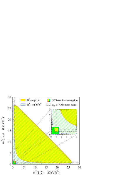
Figure 1: Dalitz plot kinematic boundaries for the $B^{0}\rightarrow\eta\pi\pi~{}$and $B^{0}\rightarrow\pi^{0}\pi^{+}\pi^{-}$ decays. The dashed (dotted) line shows the $a_{0}$ ($\rho$) mass band. The $3\Gamma$ interference regions for the $a_{0}$ (light shade) and $\rho$ (dark shade) resonances are also drawn, the region for the $a_{0}$ lying outside the allowed boundary of the $\eta\pi^{+}\pi^{-}$ Dalitz plot.

3.3 The $B\rightarrow a_{0}\rho$ Four-Body Analysis

The modes $B^{0}\to a_{0}^{+}\rho^{-}$, $B^{0}\to a_{0}^{-}\rho^{+}$ and $B^{0}\to a_{0}^{0}\rho^{0}$ decay into the common four-body final state $\eta\pi^{+}\pi^{-}\pi^{0}$. If interference between $a_{0}$’s and $\rho$’s is strong enough, one could perform a similar time and phase-space dependent analysis as for $B\rightarrow\rho\pi$.

To quantify the strength of the interference, the following parameter $\!{}^{{\bf?}}$ can be evaluated:

$$\epsilon=|\sum_{i=1}^{3}f_{i}|^{2}\Big{/}\sum_{i=1}^{3}|f_{i}|^{2}-1~{},$$ (11)

where $f_{1}=f(a_{0}^{+})f(\rho^{-})\cos\theta$, $f_{2}=f(a_{0}^{-})f(\rho^{+})\cos\theta$, and $f_{3}=f(a_{0}^{0})f(\rho^{0})\cos\theta$ are the products of the $a_{0}$ and $\rho$ Breit-Wigners, taking into account the distribution of the helicity angle $\theta$ (defined as the angle between the $\rho$ decay axis in the $\rho$ rest frame and the direction of the $\rho$ in the laboratory frame). Using simple relativistic Breit-Wigner parameterizations for the $\rho$ and the $a_{0}$ resonances, the $\epsilon$ parameter distribution is computed using $B\rightarrow a_{0}\pi$ Monte Carlo events. The mean value of $|\epsilon|$ is equal to $\sim 10\%$, corresponding to roughly half of what is observed in $B\rightarrow\rho\pi~{}$ $\!{}^{{\bf?}}$. Therefore the $B\rightarrow a_{0}\rho$ decay provides only limited interference effects.

Additional complication of having to reconstruct an extra neutral particle makes this channel less accessible than $B\to\rho\pi$. Nevertheless, the time and phase-space dependent analysis of the $B^{0}\to a_{0}\rho$ decay provides an independent and complementary way of measuring the angle $\alpha$ without any ambiguities.

3.4 The $B\rightarrow a_{0}\pi(\rho)$ Two-Body Time-Dependent Analyses

Since the $B^{0}\rightarrow\eta\pi\pi~{}$three-body final state does not exhibit interference in the Dalitz plot, one is led to a two-body analysis, i.e. where $B^{0}\rightarrow a_{0}^{+}\pi^{-}$ and $B^{0}\rightarrow a_{0}^{-}\pi^{+}$ decays are considered as two-body final states. The analysis can be applied to $B\rightarrow a_{0}\rho$ as well.

The time-dependent amplitudes for the two-body decays $B^{0}(\Delta t)\rightarrow a_{0}^{+}\pi^{-}$ and $B^{0}(\Delta t)\rightarrow a_{0}^{-}\pi^{+}$ (as well as for the CP-eigenstate $B^{0}\rightarrow a_{0}^{0}\rho^{0}$) read:

$$A(B^{0}(\Delta t)\rightarrow a_{0}^{+}\pi^{-})\propto e^{-\frac{\Gamma|\Delta t|}{2}}$$

$${}\times\left[\cos(\frac{\Delta m\Delta t}{2})A^{+-}+i~{}\sin(\frac{\Delta m\Delta t}{2})\overline{A}^{+-}\right]$$ (12)

$${}A(B^{0}(\Delta t)\rightarrow a_{0}^{-}\pi^{+})=e^{-\frac{\Gamma|\Delta t|}{2}}$$

$${}\times\left[\cos(\frac{\Delta m\Delta t}{2})A^{-+}+i~{}\sin(\frac{\Delta m\Delta t}{2})\overline{A}^{-+}\right]~{},$$ (13)

where the cosine and sine terms describe the $B^{0}\overline{B^{0}}$ flavor mixing, and $\Delta t$ is the difference of decay time between the two $B$ mesons produced at the $\Upsilon(4S)$ resonance in an asymmetric B factory. The $A^{+-}$, $A^{-+}$, $\overline{A}^{+-}$ and $\overline{A}^{-+}$ amplitudes are defined in Eqs. (2)-(9).

The time-dependent decay rate is obtained by squaring Eqs. (12) and (13), which leads to terms proportional to $\sin^{2}(\Delta m\Delta t/2)$, $\cos^{2}(\Delta m\Delta t/2)$ and $\sin(\Delta m\Delta t)$:

$$\Gamma(B^{0}(\Delta t)\rightarrow a_{0}^{\pm}\pi^{\mp})\propto e^{-\Gamma|\Delta t|}$$

$${}\times\left[{\cal A}^{\pm}_{1}\sin^{2}(\frac{\Delta m\Delta t}{2})+{\cal A}^{\pm}_{2}\cos^{2}(\frac{\Delta m\Delta t}{2})+{\cal A}^{\pm}_{3}\sin(\Delta m\Delta t)\right]$$

$${}\propto e^{-\Gamma|\Delta t|}\left[{\cal A^{\prime}}^{\pm}_{1}+{\cal A^{\prime}}^{\pm}_{2}\cos(\Delta m\Delta t)+{\cal A}^{\pm}_{3}\sin(\Delta m\Delta t)\right]~{},$$ (14)

where the ${\cal A}^{\pm}_{1,2,3}$, ${\cal A^{\prime}}^{\pm}_{1,2}$ terms are combinations of the $a_{0}^{\pm}\pi^{\mp}$ amplitudes.

Therefore, each time-dependent $B^{0}\rightarrow a_{0}^{+}\pi^{-}(\rho^{-})$, $B^{0}\rightarrow a_{0}^{-}\pi^{+}(\rho^{+})$ and $B^{0}\rightarrow a_{0}^{0}(\rho^{0})$ measurement provides three observables: ${\cal A^{\prime}}_{1}$, ${\cal A^{\prime}}_{2}$ and ${\cal A}_{3}$.

The measurement of the branching ratios for charged $B$ decays $B^{\pm}\rightarrow a_{0}\pi$$(\rho)$ and/or for the neutral final state $B^{0}\rightarrow a_{0}^{0}\pi^{0}(\rho^{0})$ each provides one observable. Using isospin invariance $\!{}^{{\bf?},{\bf?},{\bf?}}$, one can link the penguin and tree contributions from neutral and charged B decays, which provides the missing pieces for the extraction of $\alpha$:

$$\sqrt{2}\left[T^{+0}+T^{0+}\right] = T^{+-}+T^{-+}+2T^{00}~{},$$ (15)

$$P^{00} = -\frac{1}{2}(P^{+-}+P^{-+})~{},$$ (16)

$$P^{+0} = \frac{1}{\sqrt{2}}(P^{+-}-P^{-+})~{},$$ (17)

$$P^{0+} = -\frac{1}{\sqrt{2}}(P^{+-}-P^{-+})~{}.$$ (18)

Table 1 gives a comparison of the number of observables and unknowns for $B\rightarrow a_{0}\pi$, $B\rightarrow a_{0}\rho$, $B\rightarrow\rho\pi~{}$and $B\rightarrow\pi\pi~{}$analyses. Three analyses steps are described: in the upper part of the table, only charged final states of neutral $B$ decays are used. In the middle part, neutral final states of neutral $B$ decays are added. In the lower part, both neutral and charged $B$ decays are taken into account. Available isospin relations are indicated at each analyses stage.

Channel	Contributing	$a_{0}\pi$		$a_{0}\rho$		$\rho\pi$		$\pi\pi$
Ex: $B\rightarrow a_{0}\pi$	T & P Amplitudes	${\cal O}$	${\cal U}$	${\cal O}$	${\cal U}$	${\cal O}$	${\cal U}$	${\cal O}$	${\cal U}$
$\matrix{B^{0}\rightarrow a_{0}^{+}\pi^{-}\\ \overline{B^{0}}\rightarrow a_{0}^{+}\pi^{-}}$	$\matrix{e^{-i\alpha}T^{+-}+P^{+-}\\ e^{+i\alpha}T^{-+}+P^{-+}}$	3t	$\matrix{5\\ 4}$	3t	$\matrix{5\\ 4}$	3t	$\matrix{5\\ 4}$	3t	$\matrix{5\\ $-$}$
$\matrix{B^{0}\rightarrow a_{0}^{-}\pi^{+}\\ \overline{B^{0}}\rightarrow a_{0}^{-}\pi^{+}}$	$\matrix{e^{-i\alpha}T^{-+}+P^{-+}\\ e^{+i\alpha}T^{+-}+P^{+-}}$	3t	-	3t	-	3t	-	-	-
Overall norm. & phase		$-$1	$-$2	$-$1	$-$2	$-$1	$-$2	$-$1	$-$2
SCCFT ($T^{+-}=0$)		$-$1	$-$2	$-$1	$-$2
Total using only $B^{0}$’s		4 vs 5		4 vs 5		5 vs 7		2 vs 3
$\matrix{B^{0}\rightarrow a_{0}^{0}\pi^{0}\\ \overline{B^{0}}\rightarrow a_{0}^{0}\pi^{0}}$	$\matrix{e^{-i\alpha}T^{00}+P^{00}\\ e^{+i\alpha}T^{00}+P^{00}}$	$\matrix{1_{i}\\ 1_{i}}$	$\matrix{4\\ $-$}$	3t	$\matrix{4\\ $-$}$	3t	$\matrix{4\\ $-$}$	$\matrix{1_{i}\\ 1_{i}}$	$\matrix{4\\ $-$}$
Isospin relation (15)			$-$2		$-$2		$-$2		$-$2
Total adding neutral final state		6 vs 7		7 vs 7		8 vs 9		4 vs 5
$\matrix{B^{+}\rightarrow a_{0}^{+}\pi^{0}\\[0.8pt] B^{+}\rightarrow a_{0}^{0}\pi^{+}}$	$\matrix{e^{-i\alpha}T^{+0}+P^{+0}\\ e^{-i\alpha}T^{0+}+P^{0+}}$	$\matrix{1_{i}\\ 1_{i}}$	$\matrix{4\\ 4}$	$\matrix{1_{i}\\ 1_{i}}$	$\matrix{4\\ 4}$	$\matrix{1_{i}\\ 1_{i}}$	$\matrix{4\\ 4}$	$\matrix{1_{i}\\ $-$}$	$\matrix{4\\ $-$}$
$\matrix{B^{-}\rightarrow a_{0}^{-}\pi^{0}\\[0.8pt] B^{-}\rightarrow a_{0}^{0}\pi^{-}}$	$\matrix{e^{+i\alpha}T^{+0}+P^{+0}\\ e^{+i\alpha}T^{0+}+P^{0+}}$	$\matrix{1_{i}\\ 1_{i}}$	-	$\matrix{1_{i}\\ 1_{i}}$	-	$\matrix{1_{i}\\ 1_{i}}$	-	$\matrix{1_{i}\\ $-$}$	-
Isospin relations (16)-(17)			$-6$		$-6$		$-6$		$-4$
Total adding charged $B$’s		10 vs 9		11 vs 9		12 vs 11		6 vs 5

Table 1: Number of observables (${\cal O}$) and unknowns (${\cal U}$) involved in the $B\rightarrow a_{0}\pi$ and $B\rightarrow a_{0}\rho$ analyses compared to the $B\rightarrow\rho\pi~{}$and $B\rightarrow\pi\pi~{}$analyses. Upper part: charged final states of neutral $B$ decays. Middle part: neutral final states of neutral $B$ decays. Lower part: charged $B$ decays. The time-dependence of neutral $B$ decays yields three observables (cf Eq. (14)) indicated with a “t” subscript, whereas the “i” subscript corresponds to time-integrated measurements (yielding a single observable). The fact that one can exchange the two pions in the $B\rightarrow\pi\pi~{}$final state removes half of the contribution to the number of observables and unknowns. An overall normalization and phase are subtracted from the number of unknowns, and a normalization is subtracted from the number of observables. The SCCFT argument applies to the $B\rightarrow a_{0}\pi$ and $B\rightarrow a_{0}\rho$  channels, removing one observable (because two of them turn out to measure the same quantity) and two unknowns. The number of constraints coming from isospin relations is given when available. The total number of observables vs unknowns is indicated with bold characters when the fit is constrained.

The leading contribution to $B^{0}\rightarrow a_{0}^{+}\pi^{-}$ , the $T^{+-}$ tree, is suppressed by SCCFT. One of the two contributions to the color-suppressed $T^{00}$ amplitude is removed by the same SCCFT argument, but the other contribution remains. The leading contribution to the $T^{+0}$ amplitude is removed by SCCFT, but a color-suppressed contribution remains.

The number of unknowns is given by the sum of tree and penguin complex amplitudes involved at each analyses stage, plus the angle $\alpha$. One unphysical overall phase and one irrelevant overall normalization constant are subtracted from the total.

The number of observables available from a time dependent measurement is three (cf Eq. (14)), and one for the time integrated measurement. The overall normalization is subtracted from the sum of observables.

Using only the charged final states of the neutral $B$ decays does not provide enough observables to constrain $\alpha$  in any of the four analyses considered. Nevertheless, using a single theoretical prediction for an amplitude (or a ratio of amplitudes) in four-parameter $B\rightarrow a_{0}\pi(\rho)$ and two-parameter $B\rightarrow\pi\pi~{}$fits would be enough to extract the value of $\alpha$. Such a model-dependent approach can be performed with low statistics.

Adding the neutral final states does not further constrain the fits, either for $B\rightarrow a_{0}\pi$, or for $B\rightarrow\rho\pi~{}$, $B\rightarrow\pi\pi~{}$. In contrast, the $B\rightarrow a_{0}\rho$ analysis does improve, since time-dependence is observable and SCCFT holds, though the fit is only barely constrained (seven observables vs  seven unknowns).

Adding charged $B$ decays in the analyses allows all four fits to converge, but with differing robustness: whereas the $B\rightarrow\rho\pi~{}$ two-body analysis consists of an eleven-parameter fit with one extra constraint, in the $B\rightarrow a_{0}\pi$ analysis, SCCFT decreases the number of parameters to nine, with one extra constraint. As a consequence, SCCFT makes the $B\rightarrow a_{0}\pi$ analysis more robust. The $B\rightarrow a_{0}\rho$ analysis invokes a nine-parameter fit with two extra constraints, and finally, being a CP eigenstate, the $B\rightarrow\pi\pi~{}$analysis is the simplest and is performed via a five-parameter fit.

Similarly to the $B\rightarrow\pi\pi~{}$analysis, the requirement to measure the $B^{0}\rightarrow a_{0}^{0}\pi^{0}$ branching ratio makes the $B\rightarrow a_{0}\pi$ analysis far more difficult.

3.5 Mirror Solutions

CP violation in channels that benefit from SCCFT arises from interference between tree and penguin diagrams. Consequently, one measures $\alpha$-dependent terms like $\sin\alpha$ and $\cos\alpha$. This is different from the $B\rightarrow\rho\pi~{}$analysis where tree-tree interferences dominate and result in terms like $\sin 2\alpha$ and $\cos 2\alpha$.

The extraction of $\alpha$ via $B\rightarrow a_{0}\pi$ is done through terms like $\sin(\alpha+\delta)$ and $\sin(\alpha-\delta)$, where $\delta$ is a strong phases difference. It thus leads to multiple mirror solutions for $\alpha$ in the interval $[0,\pi]$, as in the two-body analyses of $B\rightarrow\pi\pi~{}$and $B\rightarrow\rho\pi~{}$.

In general, the number of mirror solutions depends on the type of analysis (e.g., one solution for the time-dependent Dalitz plot approach in $B\rightarrow\rho\pi~{}$, but eight solutions for the $B\rightarrow\pi\pi~{}$isospin analysis). To overcome this difficulty, the angle $\alpha$ has to be measured independently in various channels.

3.6 Possible Enhancement of Direct CP Violation

Even though direct CP violation is most frequently searched for with charged $B$ mesons, neutral $B$ decays can also be used to look for possible asymmetries in untagged sample:

$${\cal B}(B^{0}\to a_{0}^{+}\pi^{-}) + {\cal B}(\overline{B^{0}}\to a_{0}^{+}\pi^{-})\neq$$ (19)

$${\cal B}(B^{0}\to a_{0}^{-}\pi^{+}) + {\cal B}(\overline{B^{0}}\to a_{0}^{-}\pi^{+})~{},$$ (20)

as well as in the tagged sample:

$${\cal B}(\overline{B^{0}}\to a_{0}^{+}\pi^{-})\neq{\cal B}(B^{0}\to a_{0}^{-}\pi^{+})~{}.$$ (21)

Indeed, the suppression of the leading tree due to SCCFT may enhance direct CP violation, provided that the remaining $T^{-+}$ and $P^{-+}$ are of comparable magnitude. Similarly, in the charged $B$ decays, the interference of the remaining color-suppressed tree ($T^{+0}$) and the non-dominant tree ($T^{0+}$) with penguin contributions may enhance direct CP violating effects.

In contrast to the extraction of $\alpha$, the enhancement of direct CP violation in the $B\rightarrow a_{0}\pi$  channel does not depend on the hypotheses made in Sec. 2 (factorization and neglecting $u$- and $c$-penguin contributions), since a failure of the latter would not re-establish the hierarchy between dominant trees and penguins. The possible enhancement of direct CP violation only stems from the absence of second class currents which is experimentally established.

4 Likelihood Analysis

To assess the sensitivity to $\alpha$, and to probe the effects of non-factorizable contributions, the four time-dependent (Eq. 14) and six time-independent measurements (see table 1) are implemented in a likelihood analysis. For this toy experiment, tree and penguin amplitudes are assumed to be the same as for the $B\rightarrow\rho\pi~{}$mode (apart for the SCCFT tree $T^{+-}$) as in Ref. $\!{}^{{\bf?}}$, and $\alpha$ is taken to be equal to 1.35 rad. These values determine in particular the position of the mirror solutions. The analysis assumes a total of $1500$ events, which roughly corresponds to an integrated luminosity of $500\ fb^{-1}$, with a typical selection efficiency of $10\%$.

The SCCFT effect is described by a factor $f$ applied to the $T^{+-}$ contribution of Ref. $\!{}^{{\bf?}}$:

$$T^{+-}_{\rm a_{0}\pi}=f\times T^{+-}_{\rm\rho\pi},$$ (22)

where $f=0$ corresponds to naive factorization and a non-zero $f$ value mimics non-factorizable contributions. The analysis of the events generated with this set of amplitudes (where $f$ varies, e.g., from $0$ to $20\%$) relies on the factorization hypothesis, i.e. , $f=0$.

Figure 2: Upper plot: $chi^{2}(\alpha)=-2\ln{\cal L}$ functions for different values of $f$, the factor applied to the $B\rightarrow\rho\pi~{}$$T^{+-}$ tree to mimic non-factorizable contributions to $B\rightarrow a_{0}\pi$$f=0$ corresponds to naive factorization. A mirror solution nearly degenerate with the main mininum is observed at $\alpha\simeq 2.2$ rad. The minimum of the mirror solution becomes more pronounced as $f$ increases. For large values of $f$, it becomes a global minimum. Lower plot: Position of one of the local minima (the one located on the true value of $\alpha$ for $f=0$.) as a function of $f$.

Figure  2 shows the effects of non-factorizable contributions on the likelihood fit. The upper plot displays $\chi^{2}=-2\ln{\cal L}$ functions for $f=0$ and $f=0.1$. By construction, for $f=0$, a minimum is located at the true value of $\alpha$: this is because an analytical expression is used for the likelihood. A pronounced mirror solution is visible for $\alpha\simeq 2.2$ rad. For increasing values of $f$, this mirror solution deepens and evolves toward a global minimum. The lower plot illustrates the variation with $f$ of the local minimum corresponding to the true value of $\alpha$ for $f=0$.

In view of the non-trivial shape of $\chi^{2}(\alpha)$ on figure  2, one should not express the measurement of $\alpha$  in term of a central value and a statistical error derived from $\Delta\chi^{2}(\alpha)=1$. Instead, one should rather provide confidence levels as a function of $\alpha$ $\!{}^{{\bf?}}$. Notwithstanding the above remark, half of the range defined by $\Delta\chi^{2}(\alpha)\leq 1$ leads to $\sigma(\alpha)=0.23$ rad. This value should be compared to the systematic effect induced by the non-factorizable contributions: for, e.g., $f=0.1$, the bias in $\alpha$ is $0.18$ rad, which is comparable to the statistical error.

5 Other Charmless $B$ Decays related to SCCFT

5.1 Non-Resonant $B\to\eta\pi\pi$ Decay

The non-resonant $B\to\eta\pi\pi$ decay is affected by the absence of the second-class current as well: the coupling $W\to\eta\pi$ remains forbidden since the $\eta\pi$ state is always produced with a natural spin-parity. As for $B\rightarrow a_{0}\pi$, this can lead to an enhancement of direct CP violation.

Since the spin-parities of $\eta^{\prime}(958)$ and $\eta(550)$ are identical, both $B^{0}\to\eta\pi^{+}\pi^{-}$ and $B^{0}\to\eta^{\prime}(958)\pi^{+}\pi^{-}$ decays should be considered. Contributions from channels like $B^{0}\to\eta(\eta^{\prime})\rho^{0}$ contaminate the non-resonant signal sample, and have to be vetoed.

5.2 $B\rightarrow a_{0}\pi$ vs $a_{0}K$

As in $B\rightarrow\pi\pi~{}$  the measurement of the ratio of ${\cal B}(B^{0}\rightarrow a_{0}\pi)/{\cal B}(B^{0}\rightarrow a_{0}K)$, under some assumptions (e.g., neglecting the Cabibbo suppressed tree contribution in the $B^{0}\to a_{0}K$ decay), can help to estimate the ratio of tree to penguin contributions to the $B\rightarrow a_{0}\pi$ decay. It also gives a handle on the charming penguin contributions.

5.3 Analysis of $B^{0}\to b_{1}\pi$

The $b_{1}$ resonance, with even $G$-parity and odd spin-parity, has the same properties leading to SCCFT as the $a_{0}$, so that the two-body analysis for $\alpha$  can be performed accordingly.

Since the reconstruction of the $b_{1}$ proceeds through the decays $b_{1}\to\omega\pi\to 3\pi^{\pm}\pi^{0}$, the higher multiplicity of the final state and the lower energy of the $\pi^{0}$ renders this mode less accessible. In addition, feed-through from $W\to\omega\pi$ from the $J^{P}=1^{-}$ channel contaminates the $b_{1}(\omega\pi)\pi$ signal. On the other hand, the narrow $b_{1}$ and $\omega$ resonances and the helicity distribution improve the background suppression.

Finally, the non-resonant $W\to\omega\pi$ transition can be produced in a $G$-parity allowed state due to the spin $1$ of the $\omega$. Therefore, direct CP searches in the non-resonant $B\rightarrow\omega\pi\pi$ do not benefit from the absence of second class currents.

5.4 Pure Penguin $a_{0}a_{0}$, $b_{1}b_{1}$ and $a_{0}b_{1}$ Decays

Due to the absence of Second Class Currents, the decays $B^{0}\to a_{0}a_{0}$, $B^{0}\to b_{1}b_{1}$ and $B^{0}\to a_{0}b_{1}$ (to both charged and neutral final states, the latter being Fierz-transformed of the former) proceed via penguins only. Therefore, there should not be any direct CP violation in these decays, unless if other contributions carrying a different weak phase are present ($u$- and $c$-penguins, re-scattering from other final states). The observation of direct CP violation in these decays thus provides a direct measurement of the non-factorizable contributions.

Similarly, the corresponding charged $B$ tree decays (including the color-suppressed ones, due to Fierz-transformation) are suppressed by both the absence of Second Class Currents and isospin conservation (Eq. 15). The gluonic ($u$-, $c$- and $t$-) penguin contributions to $B^{\pm}\to a_{0}^{\pm}a_{0}^{0}$ and $B^{\pm}\to b_{1}^{\pm}b_{1}^{0}$ are suppressed by isospin conservation when inserting the relation $P^{+-}=P^{-+}$ in Eq. (18). Hence, since both tree and gluonic penguin contributions are suppressed, the observation of the $B^{\pm}\to a_{0}^{\pm}a_{0}^{0}$ and $B^{\pm}\to b_{1}^{\pm}b_{1}^{0}$ decays provides again a measurement of the non-factorizable contributions.

Moreover, the time-dependent analysis of $B^{0}\to a_{0}b_{1}$ allows the extraction of the strong phase difference between the two penguin amplitudes $P^{+-}$ and $P^{-+}$. Nevertheless, since the $B\to a_{0}b_{1}$ decay has one $\eta$ and four charged $\pi$ in the final state, the extraction of the signal is marred by large combinatorial background.

5.5 Decays into Higher Spin Mesons

Due to angular momentum conservation, there is no coupling of virtual W to the hadronic states of spin larger than one. The corresponding tree diagrams do not contribute to the decay amplitude thus causing effects similar to those created by SCCFT.

One example of such decays is $B^{0}\to a_{2}(1320)\pi\to\eta\pi\pi$. Other higher resonance excitations could be considered for similar analyses to those described in this article.

6 Conclusion

Constraints imposed by the absence of second class currents provide new opportunities for CP violation studies in charmless $B$ decays. In this article, we discussed how the CKM angle $\alpha$ can be extracted from analyses of $B$ decays into the final states $a_{0}\pi(\rho)$ in a more robust fashion than in the original isospin-pentagon analyses proposed for $B\rightarrow\rho\pi~{}$and $B\rightarrow\pi\pi~{}$. A similar analysis can be performed for the decays $b_{1}\pi$ and $\eta(\eta^{\prime})\pi\pi$, but these latter modes are experimentally more challenging. Fits with four (if one theoretical amplitude or one ratio of amplitudes is added) to nine (with no such theoretical input) parameters can be performed for each of these decays. A fit combining several channels would reduce the number of mirror solutions, and decrease the error on $\alpha$.

Significant enhancement of direct CP asymmetries could arise in the following channels: $B\rightarrow a_{0}\pi$, $B\rightarrow b_{1}\pi$ and non-resonant $B\to\eta(\eta^{\prime})\pi\pi$ due to the absence of second class currents, independently of the hypotheses needed for the extraction of $\alpha$  (i.e. , factorization and the neglect of $u$- and $c$-penguins).

Finally, many of these decays can be used to test the factorization assumption, and measure the non-factorizable contributions. For a luminosity of the order of about $500fb^{-1}$, the systematic bias on $\alpha$ , induced by non-factorizable contributions of the size of $10\%$, remains of the same order than the statistic uncertainty.

Remark

Factorization breaking can be studied in $B\rightarrow a_{0}\pi$ as described in this article, and in a variety of other decays, following the idea that the suppression of factorizable contributions allows to study the non-factorizable ones. CP-violation studies (measurement of $2\beta+\gamma$ and enhanced CP assymetries) can also been performed in these decays. This has been independently described in two articles by M. Diehl and G. Hiller $\!{}^{{\bf?}}$.

References

• [1] A.E. Snyder, H.R. Quinn, Phys.Rev.D 48 (1993) 2139
• [2] M. Gronau and D. London, Phys.Rev.Lett. 65 (1990) 3381
• [3] H.J. Lipkin, Y. Nir, H.R. Quinn, A.E. Snyder, Phys.Rev.D 44 (1991) 1454
• [4] A.S. Dighe, C.S. Kim , Phys.Rev.D 62 (2000) 111302
• [5] A. Lyon for the CLEO collaboration, β€œCP Violation Studies with Rare B Physics at CLEO”, talk given at BCP4, Ise-Shime, Japan, Feb.19-23, 2001
• [6] T.J. Champion for the BABARΒ  collaboration, to be published in the proceedings of 30th International Conference on High-Energy Physics (ICHEP 2000), Osaka, Japan, 27 Jul - 2 Aug 2000. SLAC-PUB-8696, BABAR-PROC-00-13, hep-ex/0011018
• [7] S.VersillΓ©, La violation de CP dans BaBar: Γ©tiquetage des mΓ©sons B et Γ©tude du canal $B\to 3\pi$, PhD thesis (in French), UniversitΓ© de Paris Sud (1999)
• [8] The branching ratio of $B0\rightarrow a_{0}^{\pm}\pi^{\mp}$ has been recently measured by the BABAR collaboration:
B.Β Aubert et al, β€œSearch for $B0\rightarrow a_{0}(980)\pi$”, July 2001, hep-ex/0107075
• [9] Particle Data Group, C.Caso et al, Eur.Phys.JΒ C3 (2000) 1
• [10] J.Β Charles, Phys.Rev.D 59 (1999) 054007
• [11] BABARΒ  Collaboration, The BABARΒ  Physics Book (1998)
• [12] M.Β Diehl and G.Β Hiller, SLAC-PUB-8822, DESY-01-060, hep-ph/0105194 Published in JHEP 0106:067,2001
M.Β Diehl and G.Β Hiller, SLAC-PUB-8837, DESY-01-061, hep-ph/0105213