CLNS 01/1737

hep-ph/0105217
May 21, 2001

Improved Determination of $|V_{ub}|$ from Inclusive Semileptonic $B$-Meson Decays

Thomas Becher and Matthias Neubert

Newman Laboratory of Nuclear Studies, Cornell University
Ithaca, NY 14853, USA

We reduce the perturbative uncertainty in the determination of $|V_{ub}|$ from inclusive semileptonic $B$ decays by calculating the rate of $B\to X_{u}\,l\,\nu$ events with dilepton invariant mass $\sqrt{q^{2}}>M_{B}-M_{D}$ at subleading order in the hybrid expansion, and to next-to-leading order in renormalization-group improved perturbation theory. We also resum logarithmic corrections to the leading power-suppressed contributions. Studying the effect of different $b$-quark mass definitions we find that the branching ratio after the cut is $\mbox{Br}(B\to X_{u}\,l\,\nu)=(20.9\pm 4.0)\,|V_{ub}|^{2}$, where the dominant error is due to the uncertainty in the $b$-quark mass. This implies that $|V_{ub}|$ can be determined with a precision of about 10%.

1 Introduction

The total inclusive, semileptonic $B\to X_{u}\,l\,\nu$ decay rate admits a clean theoretical analysis based on the heavy-quark expansion. The optical theorem is used to relate the decay rate to the forward matrix element of the product of two hadronic currents, which is evaluated using the operator product expansion [1, 2, 3]. The total rate is presently known including corrections of order $\alpha_{s}^{2}$ [4] and $\Lambda^{2}/m_{b}^{2}$ (with $\Lambda$ a typical hadronic scale). An accurate knowledge of the total rate does not immediately translate into a precise determination of $|V_{ub}|$, since experimentally one has to impose cuts on the kinematical variables in order to discriminate the $b\to u$ transitions against the much larger $B\to X_{c}\,l\,\nu$ background. The first inclusive determination of $|V_{ub}|$ was based on a measurement of the charged-lepton energy spectrum in the endpoint region, which is kinematically forbidden for decays with a charm meson in the final state. This cut eliminates about 90% of the signal. It is difficult to reliably calculate the remaining event fraction, since the operator product expansion breaks down in this part of the phase space and must be replaced by a twist expansion [5, 6].

Recently, it was shown that the situation is improved when a cut $q^{2}>q_{0}^{2}$ with $q_{0}^{2}\geq(M_{B}-M_{D})^{2}$ is applied to the dilepton invariant mass [7]. This keeps about 20% of the signal events, and the fraction of the remaining events can be calculated in a model-independent way using the operator product expansion. After the cut, the typical momentum flow $\mu_{c}$ through the hadronic tensor is of order the charm-quark mass or less, so that the problem at hand involves the three scales $m_{b}>\mu_{c}>\Lambda$. In the standard heavy-quark expansion, the charm and the $b$-quark masses are treated on the same footing, but it is known that the convergence of this expansion at the charm scale can be poor. In this letter we follow the strategy proposed in [8] and perform a two-step expansion (the “hybrid expansion”) in the ratios $\mu_{c}/m_{b}$ and $\Lambda/\mu_{c}$. The first step is to integrate out the degrees of freedom above the scale $\mu_{c}$ and to sum up logarithms of the form $\alpha_{s}\ln(\mu_{c}/m_{b})$ using the renormalization group (RG). This is achieved by expanding the weak currents and the QCD Lagrangian to order $1/m_{b}$ in the heavy-quark effective theory (HQET) [9], and calculating the Wilson coefficients of the pertinent operators at next-to-leading order (NLO) in RG-improved perturbation theory. Whereas the Wilson coefficients of the leading-order currents [10, 11] and of the $O(1/m_{b})$ corrections to the HQET Lagrangian [12, 13] were known for a long time, the NLO calculation of the coefficients entering the expansion of the currents at order $1/m_{b}$ was completed only recently [14, 15, 16, 17].

In the present work, we perform the second step in the hybrid expansion and construct the operator product expansion in the resulting low-energy effective theory. We calculate the decay rate $\Gamma(B\to X_{u}\,l\,\nu)|_{q^{2}>q_{0}^{2}}$ at subleading order in the ratio $\mu_{c}/m_{b}$ and to NLO in RG-improved perturbation theory. We also resum leading logarithmic corrections to the power corrections of order $(\Lambda/\mu_{c})^{2}$. In contrast with previous analyses [7, 8] we calculate the decay rate directly, rather than calculating the fraction of events that passes the $q^{2}$-cut and then multiplying this fraction with an independent result for the total semileptonic rate. Since the characteristic scale of the total rate is significantly higher than (and parametrically different from) the typical hadronic scale $\mu_{c}$ after the $q^{2}$-cut, the theoretical error cannot be reduced by separating the two calculations. Based on a detailed analysis of the residual renormalization-scale dependence and the sensitivity to the definition of the $b$-quark mass, we conclude that the $B\to X_{u}\,l\,\nu$ branching ratio after the dilepton invariant-mass cut can be calculated reliably, allowing for a determination of $|V_{ub}|$ at the 10% level.

2 Construction of the hybrid expansion

A cut $q^{2}>q_{0}^{2}$ on the dilepton invariant mass squared $q^{2}=(p_{l}+p_{\nu})^{2}$ implies

$$M_{X}\leq E_{X}\leq\frac{1}{2M_{B}}\left(M_{B}^{2}+M_{X}^{2}-q_{0}^{2}\right)\,,\qquad M_{\pi}^{2}\leq M_{X}^{2}\leq\Big{(}M_{B}-\sqrt{q_{0}^{2}}\Big{)}^{2}$$ (1)

for the hadronic invariant mass $M_{X}$ and energy $E_{X}$. For $q_{0}^{2}=(M_{B}-M_{D})^{2}$ both variables vary between $M_{\pi}$ and $M_{D}$, and thus no charmed hadrons are allowed in the final state. If the cutoff is chosen higher (as may be required for experimental reasons), the maximal values of $M_{X}$ and $E_{X}$ become less than the $D$-meson mass. The kinematical variables that enter the partonic calculation of the decay rate are the parton invariant mass and energy, $\sqrt{p^{2}}$ and $v\cdot p$, where $p=m_{b}\,v-q$ with $v$ being the velocity of the $B$-meson. It is convenient to work with the dimensionless quantities $\xi=p^{2}/(v\cdot p)^{2}$ and $z=2v\cdot p/m_{b}$, the phase space for which is

$$0\leq\xi\leq 1\,,\qquad 0\leq z\leq z_{\rm max}=\frac{2}{\xi}\Big{(}1-\sqrt{1-2\delta\,\xi}\Big{)}\,.$$ (2)

While $\xi$ is of order unity, independent of the value of $q_{0}^{2}$, the quantity $z$ is parametrically suppressed by

$$\delta=\frac{\mu_{c}}{m_{b}}\,,\qquad\text{with}\qquad\mu_{c}=\frac{m_{b}^{2}-q_{0}^{2}}{2m_{b}}\,.$$ (3)

With the optimal value $q_{0}^{2}=(M_{B}-M_{D})^{2}\simeq(m_{b}-m_{c})^{2}$ the characteristic scale of the parton momenta is $\mu_{c}\sim m_{c}$.

The strong-interaction dynamics of the inclusive decay $B\to X_{u}\,l\,\nu$ is encoded in the imaginary part of the hadronic tensor $T_{\mu\nu}$ defined as

$$T_{\mu\nu}(p,v) = \frac{1}{i}\int d^{4}x\,e^{i(p-m_{b}v)\cdot x}\,\frac{1}{2M_{B}}\,\langle B(v)|\,\text{\bf T}\left\{J_{\mu}^{\dagger}(x),J_{\nu}(0)\right\}|B(v)\rangle$$ (4)

$$= \left(p_{\mu}v_{\nu}+v_{\mu}p_{\nu}-g_{\mu\nu}\,v\cdot p-i\epsilon_{\mu\nu\alpha\beta}\,p^{\alpha}v^{\beta}\right)\,T_{1}$$

$$\mbox{}-g_{\mu\nu}\,T_{2}+v_{\mu}v_{\nu}\,T_{3}+\left(p_{\mu}v_{\nu}+v_{\mu}p_{\nu}\right)\,T_{4}+p_{\mu}p_{\nu}\,T_{5}\,,$$

where the scalar functions $T_{i}$ depend on $p^{2}$ and $v\cdot p$, or equivalently, on $\xi$ and $z$. The weak current $J_{\mu}=\bar{u}\gamma_{\mu}(1-\gamma_{5})b$ mediates the $b\to u$ transition. To separate the long- and short-distance physics one usually performs the operator product expansion of the hadronic tensor and calculates the corresponding Wilson coefficient functions in perturbation theory. However, since in the present case the characteristic scale $\mu_{c}$ of the momentum flow through the operator product is lower than the $b$-quark mass, the perturbative expansion of the Wilson coefficients involves logarithms of the ratio $\mu_{c}/m_{b}$. To improve the quality of the perturbative results these logarithms should be summed. This can be achieved by absorbing the physics above the scale $\mu_{c}$ into the couplings of a low-energy effective theory.

The relevant effective theory is the HQET, and the expansion of the weak current at NLO reads [14, 15]

$$J_{\mu}=\sum_{i}C_{i}(\mu)\,O_{i}+\frac{1}{2m_{b}}\sum_{j}B_{j}(\mu)\,Q_{j}+O(1/m_{b}^{2})\,.$$ (5)

The two operators contributing at leading order are

$$O_{1}=\bar{u}_{L}\gamma_{\mu}h_{v}\,,\qquad O_{2}=\bar{u}_{L}v_{\mu}h_{v}\,,$$ (6)

where $\bar{u}_{L}\equiv\bar{u}(1+\gamma_{5})$, and $h_{v}$ is the effective heavy-quark spinor of the HQET. At NLO in $1/m_{b}$, the operator basis contains ten independent operators. Six of these are local operators involving a gauge-covariant derivative on one of the quark fields:

$$Q_{1} =\bar{q}_{L}\gamma_{\mu}i\hbox to0.0pt{\hskip 2.84544pt/\hss}{D}h_{v}\,, Q_{2} =\bar{q}_{L}v_{\mu}i\hbox to0.0pt{\hskip 2.84544pt/\hss}{D}h_{v}\,, Q_{3} =\bar{q}_{L}iD_{\mu}h_{v}\,,$$

$$Q_{4} =\bar{q}_{L}(iv\!\cdot\!D)^{\dagger}\gamma_{\mu}h_{v}\,, Q_{5} =\bar{q}_{L}(iv\!\cdot\!D)^{\dagger}v_{\mu}h_{v}\,, Q_{6} =\bar{q}_{L}(iD_{\mu})^{\dagger}h_{v}\,.$$ (7)

The remaining four involve time-ordered products of the leading-order currents with the operators $O_{\rm kin}=\bar{h}_{v}(iD)^{2}h_{v}$ and $O_{\rm mag}=\frac{g_{s}}{2}\,\bar{h}_{v}\sigma_{\mu\nu}G^{\mu\nu}h_{v}$ appearing at order $1/m_{b}$ in the HQET Lagrangian:

$$Q_{7,8}=i\int d^{4}x\,\mbox{\bf T}\,\{O_{1,2}(0),O_{\rm kin}(x)\}\,,\qquad Q_{9,10}=i\int d^{4}x\,\mbox{\bf T}\,\{O_{1,2}(0),O_{\rm mag}(x)\}\,.$$ (8)

These nonlocal operators are present because we work with eigenstates of the lowest-order HQET Lagrangian, so that all dependence on the heavy-quark mass is explicit. It is convenient to treat the operators $Q_{7,\dots,10}$ on the same footing as the local operators $Q_{1,\dots,6}$, because the nonlocal operators mix into the local ones under renormalization. We have recently completed the calculation of the two-loop anomalous dimension matrix for the operators $Q_{j}$ and solved the RG equations for their coefficients $B_{j}(\mu)$ [17].

When the expansion (5) is inserted into the operator product in (4), all dependence on the $b$-quark mass becomes explicit and is contained in the Wilson coefficients $C_{i}$, $B_{j}$ and the $1/m_{b}$ prefactor of the higher-dimension operators. In the next step, we perform the operator product expansion and obtain forward $B$-meson matrix elements of local operators of the form $\langle B(v)|\,\bar{h}_{v}\dots h_{v}\,|B(v)\rangle$ in the low-energy theory. To order $(\Lambda/\mu_{c})^{2}$, these matrix elements can be expressed in terms of the parameters [18]

$$\lambda_{1}=\frac{1}{2M_{B}}\,\langle B|\,O_{\rm kin}\,|B\rangle\,,\qquad\lambda_{2}(\mu)=\frac{1}{6M_{B}}\,\langle B|\,O_{\rm mag}\,|B\rangle\,.$$ (9)

The anomalous dimension of the kinetic operator vanishes because of reparameterization invariance [19]. Up to higher orders in the heavy-quark expansion, $\lambda_{2}$ is determined from the mass splitting $\lambda_{2}(m_{b})\simeq\frac{1}{4}(M_{B^{*}}^{2}-M_{B}^{2})\simeq 0.12$ GeV².

By dimensional analysis, the contributions from time-ordered products of higher-dimension operators in (5) are suppressed by powers of $\delta=\mu_{c}/m_{b}$. At NLO in $\delta$, it suffices to evaluate time-ordered products with operator insertions of the type $\{O_{i},O_{j}\}$ or $\{O_{i},Q_{j}\}$. The decay rate is then obtained by contracting the result for the hadronic tensor with the lepton tensor and integrating over the portion of phase space with $q^{2}>q_{0}^{2}$:

$$\Gamma(\delta)\equiv\Gamma(B\to X_{u}\,l\,\nu)\big{|}_{q^{2}>q_{0}^{2}}=\int\limits_{0}^{1}\!d\xi\int\limits_{0}^{z_{\rm max}}\!dz\,\frac{d^{2}\Gamma}{d\xi\,dz}=\frac{1}{2\pi i}\oint\limits_{|\xi|=1}\!d\xi\int\limits_{0}^{z_{\rm max}}\!dz\,T(\xi,z)\,,$$ (10)

where $z_{\rm max}=2\delta+\delta^{2}\xi+O(\delta^{2})$ from (2). Using the fact that the hadronic tensor is an analytic function of $\xi$ apart from discontinuities on the positive real axis, we have written the expression for the rate $\Gamma(\delta)$ as a contour integral in the complex $\xi$-plane. The integrand of the contour integral is [20]

$$T(\xi,z) = \frac{\Gamma_{0}m_{b}z^{3}}{16}\sqrt{1-\xi}\,\bigg{\{}m_{b}z\Big{[}12-8z-(4-3z)z\,\xi\Big{]}\,T_{1}+6(4-4z+z^{2}\xi)\,T_{2}$$ (11)

$$\hskip 88.2037pt\mbox{}+2z^{2}(1-\xi)(T_{3}+2m_{b}\,T_{4}+m_{b}^{2}\,T_{5})\bigg{\}}\,,$$

where

$$\Gamma_{0}=\frac{G_{F}^{2}|V_{ub}|^{2}m_{b}^{5}}{192\pi^{3}}$$ (12)

is the tree-level decay rate.

Figure 1: One-loop graphs contributing to the hadronic tensor. The crossed circles represent insertions of the operators $O_{i}$ or $Q_{j}$. The solid squares in the last eight diagrams denote insertions of $O_{\rm kin}$ or $O_{\rm mag}$.

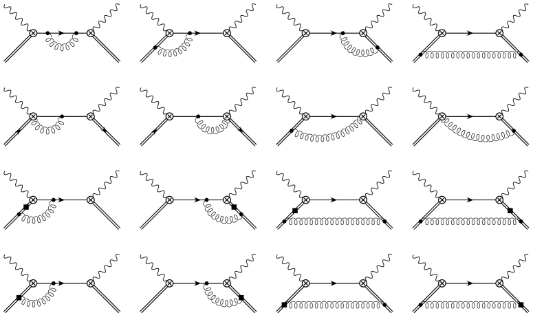
At NLO in RG-improved perturbation theory, the matrix elements of the hadronic tensor must be evaluated including corrections of order $\alpha_{s}$ in the low-energy theory. These are obtained by evaluating the contributions of all physical cuts of the diagrams shown in Figure 1. These diagrams contain infrared divergences for $\xi\to 0$ from soft and collinear gluons, which cancel once the differential rate is integrated over phase space, because the rate $\Gamma(\delta)$ is an infrared-safe quantity. The contour-integral representation in (10) avoids the singularity at $\xi=0$. After integrating over the loop momentum, the function $T(\xi,z)$ is given by an integral over Feynman parameters. At this point we exchange the order of integration and integrate over the phase space first. The $z$-integration is trivial, because the dependence of the loop integrals on $z$ is fixed by their mass dimension. Note that the upper limit $z_{\rm max}$ of the integration depends on $\xi$. After expanding to NLO in $\delta$, the $\xi$-integrals can all be reduced to

$$\big{\{}G_{\alpha}(a)\,;H_{\alpha}(a)\big{\}}=\frac{1}{2\pi i}\oint\limits_{|\xi|=1}\!d\xi\,\frac{\sqrt{1-\xi}}{(a-\xi)^{\alpha}}\,\big{\{}1\,;\frac{1}{\xi}\,\big{\}}\,,$$ (13)

where the denominator $(a-\xi)^{\alpha}$ with $a\geq 0$ is the result of the Feynman parameterization. Some of the diagrams have a pole at $\xi=0$ due to the propagation of a single $u$-quark. The integral $G_{\alpha}(a)$ evaluates to

$$G_{\alpha}(a)=-\frac{\sqrt{\pi}}{2\Gamma(\alpha)\Gamma(\frac{5}{2}-\alpha)}\,\frac{\theta(1-a)}{(1-a)^{\alpha-\frac{3}{2}}}\,.$$ (14)

The second integral picks up contributions for $a<1$ and $a>1$. It is needed only for $\alpha=1+\epsilon$ and $\alpha=\epsilon$ (with $\epsilon=2-d/2$ the dimensional regulator). We find

$$H_{1+\epsilon}(a) = \frac{\theta(1-a)}{a}\,\bigg{\{}1-\sqrt{1-a}\,\Big{[}1-\epsilon\ln 4(1-a)\Big{]}-2\epsilon\ln(1+\sqrt{1-a})+O(\epsilon^{2})\bigg{\}}$$ (15)

$$\mbox{}+\frac{\theta(a-1)}{a^{1+\epsilon}}\,.$$

We have not expanded the result for $a>1$, since we will have to integrate it from $a=1$ to $\infty$ when performing the integrals over Feynman parameters. The corresponding expression for the function $H_{\epsilon}(a)$ can be obtained by integrating the above result with respect to $a$.

We now present the results of our calculation. We expand the rate $\Gamma(\delta)$ in powers of $\delta$ and define

$$\Gamma(\delta)=16\Gamma_{0}\,\delta^{3}\left(\widehat{\Gamma}_{3}+\delta\,\widehat{\Gamma}_{4}+\delta^{2}\,\widehat{\Gamma}_{\geq 5}\right),$$ (16)

where the dimensionless expansion coefficients $\widehat{\Gamma}_{n}$ collect terms of different order in the hybrid expansion. The leading-order contribution $\widehat{\Gamma}_{3}$ was calculated in [8]; the NLO term $\widehat{\Gamma}_{4}$ is the main result of the present work. We find that

$$\widehat{\Gamma}_{3} = C_{1}(\mu)^{2}\,F_{3}[C_{1},C_{1}]\,,$$

$$\widehat{\Gamma}_{4} = \sum_{i=1,2}\,C_{1}(\mu)\,C_{i}(\mu)\,F_{4}[C_{1},C_{i}]+\sum_{j=4,6,7,9}\,C_{1}(\mu)\,B_{j}(\mu)\,F_{4}[C_{1},B_{j}]\,,$$ (17)

where ($C_{F}=4/3$ is a color factor)

$$F_{3}[C_{1},C_{1}] = 1+\frac{C_{F}\alpha_{s}(\mu)}{4\pi}\left(6\ln\frac{\mu}{2\mu_{c}}+19-\frac{8\pi^{2}}{3}\right)-\frac{3}{2}\,\frac{\lambda_{2}(\mu)}{\mu_{c}^{2}}+\dots\,,$$

$$F_{4}[C_{1},C_{1}] = -\bigg{\{}1+\frac{C_{F}\alpha_{s}(\mu)}{4\pi}\left(6\ln\frac{\mu}{2\mu_{c}}+\frac{29}{2}-\frac{8\pi^{2}}{3}\right)\bigg{\}}+\frac{3}{2}\,\frac{\lambda_{1}+3\lambda_{2}(\mu)}{\mu_{c}^{2}}+\dots\,,$$

$$F_{4}[C_{1},C_{2}] = \frac{1}{2}+\dots\,,$$

$$F_{4}[C_{1},B_{4}] = \frac{3}{4}\,\bigg{\{}1+\frac{C_{F}\alpha_{s}(\mu)}{4\pi}\left(6\ln\frac{\mu}{2\mu_{c}}+\frac{37}{2}-\frac{8\pi^{2}}{3}\right)\bigg{\}}-\frac{3}{4}\,\frac{\lambda_{2}(\mu)}{\mu_{c}^{2}}+\dots\,,$$

$$F_{4}[C_{1},B_{6}] = \frac{1}{4}\,\bigg{\{}1+\frac{C_{F}\alpha_{s}(\mu)}{4\pi}\left(6\ln\frac{\mu}{2\mu_{c}}+\frac{39}{2}-\frac{8\pi^{2}}{3}\right)\bigg{\}}+\frac{3}{4}\,\frac{\lambda_{2}(\mu)}{\mu_{c}^{2}}+\dots\,,$$

$$F_{4}[C_{1},B_{7}] = \frac{C_{F}\alpha_{s}(\mu)}{4\pi}\left(6\ln\frac{\mu}{2\mu_{c}}+\frac{9}{2}\right)-\frac{3}{2}\,\frac{\lambda_{1}}{\mu_{c}^{2}}+\dots\,,$$

$$F_{4}[C_{1},B_{9}] = \frac{1}{3}\,\frac{C_{F}\alpha_{s}(\mu)}{4\pi}\left(6\ln\frac{\mu}{2\mu_{c}}+\frac{25}{2}\right)-\frac{9}{2}\,\frac{\lambda_{2}(\mu)}{\mu_{c}^{2}}+\dots\,.$$ (18)

Note that the Wilson coefficient $C_{2}$ starts at NLO in $\alpha_{s}$, so there is no need to include $O(\alpha_{s})$ corrections to the quantity $F_{4}[C_{1},C_{2}]$. The coefficients $B_{7}=C_{1}\,C_{\rm kin}$ and $B_{9}=C_{1}\,C_{\rm mag}$ are determined in terms of products of coefficients appearing in the leading-order expansion of the currents and in the HQET Lagrangian. $C_{\rm mag}$ is the coefficient of the chromo-magnetic operator $O_{\rm mag}$, and $C_{\rm kin}=1$ is the coefficient of the kinetic operator $O_{\rm kin}$. The remaining coefficients, $B_{4}$ and $B_{6}$, were calculated at NLO in [17]. The Wilson coefficients, as well as the matrix elements in the low-energy theory, depend on the choice of the renormalization scheme. The scheme dependence cancels in the result for the decay rate $\Gamma(\delta)$. In [17] we have considered a class of renormalization schemes parameterized by the quantity $\Delta_{\rm RS}=2\ln(\mu_{\overline{\rm MS}}/\mu_{\rm RS})$. Our results (2) refer to the $\overline{\rm MS}$ renormalization scheme (with anticommuting $\gamma_{5}$). The corresponding results in a different scheme RS are obtained by replacing

$$\ln\frac{\mu_{\overline{\rm MS}}}{2\mu_{c}}\to\ln\frac{\mu_{\rm RS}}{2\mu_{c}}+\frac{\Delta_{\rm RS}}{2}\,.$$ (19)

That way, it can be checked that the scheme-dependent terms proportional to $\Delta_{\rm RS}$ indeed cancel in the final result.

The above expressions are given in terms of the $b$-quark pole mass $m_{b}\equiv m_{b}^{\text{pole}}$, which is the expansion parameter that enters in the HQET. However, this mass parameter is plagued by infrared renormalon ambiguities, and it is better to eliminate it from the final result for the decay rate. It is well known that the convergence of the perturbative series of inclusive decay rates can be improved by replacing the pole mass in favor of a low-scale subtracted quark mass, which is obtained from the pole mass by removing a long-distance contribution proportional to a subtraction scale $\mu_{f}\sim\mbox{several}\times\Lambda$ [21, 22, 23, 24]. In addition to $m_{b}$, the characteristic scale $\mu_{c}=(m_{b}^{2}-q_{0}^{2})/(2m_{b})$ of the hybrid expansion and the associated parameter $\delta=\mu_{c}/m_{b}$ depend on the definition of the quark mass. It has been shown in [8] that one should choose $\mu_{f}=\zeta\mu_{c}$ with a parameter $\zeta=O(1)$ so as not to upset the power-counting in the hybrid expansion. Specifically, we use the potential-subtracted (PS) mass $m_{b}^{\text{PS}}$ introduced by Beneke [21]. At NLO, the relation between the pole mass and the PS mass reads

$$m_{b}^{\text{pole}}=m_{b}^{\text{PS}}(\mu_{f})+\mu_{f}\,\frac{4\alpha_{s}(\mu)}{3\pi}\left\{1+\frac{\alpha_{s}(\mu)}{2\pi}\left[\beta_{0}\left(\ln\frac{\mu}{\mu_{f}}+\frac{11}{6}\right)-4\right]+\dots\right\},$$ (20)

where $\beta_{0}=11-\frac{2}{3}\,n_{f}$ is the first coefficient of the $\beta$ function. With $\mu_{f}=\zeta\mu_{c}$ it follows that

$$m_{b}^{\text{pole}}=m_{b}^{\text{PS}}(\zeta\mu_{c})\left[1+\delta\,\zeta\,\frac{4\alpha_{s}(\mu)}{3\pi}+O(\alpha_{s}^{2})\right].$$ (21)

From now on, we use the PS mass $m_{b}\equiv m_{b}^{\text{PS}}(\zeta\mu_{c})$ in all our equations unless indicated otherwise. The parameters $\mu_{c}$ and $\delta$ are defined with respect to this choice. This results in extra terms in the perturbative expansion proportional to $\zeta$. The results in the pole scheme can be recovered by setting $\zeta=0$.

In [7], the authors have eliminated the pole mass in favor of the so-called Upsilon mass $m_{b}^{\text{1S}}$ [22], which up to a small nonperturbative contribution is one half of the mass of the $\Upsilon(1S)$ resonance. The relation between the Upsilon mass and the pole mass is

$$m_{b}^{\text{pole}}=m_{b}^{\text{1S}}+\frac{2m_{b}^{\text{1S}}\alpha_{s}(\mu)^{2}}{9}\left\{1+\frac{\alpha_{s}(\mu)}{\pi}\left[\beta_{0}\left(\ln\frac{\mu}{\frac{4}{3}\,m_{b}^{\text{1S}}\alpha_{s}(\mu)}+\frac{11}{6}\right)-4\right]+\dots\right\}.$$ (22)

In higher orders in this expansion the logarithms $\ell=\ln[\mu/\frac{4}{3}\,m_{b}^{\text{1S}}\alpha_{s}(\mu)]$ appear in the form $[\ell^{n}/n!+\ell^{n-1}/(n-1)!+\dots+1]\sim\exp(\ell)$, which yields a factor $[\mu/\frac{4}{3}\,m_{b}^{\text{1S}}\alpha_{s}(\mu)]$. Hence, schematically the relation between the masses becomes

$$m_{b}^{\text{pole}}\sim m_{b}^{\text{1S}}+\mu\,\frac{\alpha_{s}(\mu)}{6}\left[1+\mbox{nonlogarithmic terms}\right]\,,$$ (23)

which shows that despite of the unusual form of (22) the Upsilon mass is a low-scale subtracted mass in the sense described earlier. (One may, however, question whether this argument can consistently be applied in low-order calculations.) Based on this observation, the authors of [22] have suggested to treat the $O(\alpha_{s}^{2})$ term on the right-hand side of (22) as an $O(\alpha_{s})$ correction when the Upsilon mass is used in the context of perturbative expansions in the $B$ system. Therefore, in our case we should replace $m_{b}^{\text{pole}}=m_{b}^{\text{1S}}[1+\frac{2}{9}\,\alpha_{s}(\mu)^{2}+\dots]$ and treat the $O(\alpha_{s}^{2})$ term as a term of order $\delta\,\alpha_{s}(\mu)$, as in (21). This means that our formulae apply without modification to the Upsilon scheme, provided we set $\zeta=\pi\alpha_{s}(\mu)/(6\delta)$ and consider this to be a parameter of order unity.

Inserting the explicit expressions for the Wilson coefficients and matrix elements into (2), and evaluating the results for $N_{c}=3$ colors and $n_{f}=4$ light quark flavors, we obtain

$$x^{-12/25}\,\widehat{\Gamma}_{3} = 1+k_{1}\,\frac{\alpha_{s}(m_{b})}{\pi}+\left(2\ln\frac{\mu}{2\mu_{c}}+4\zeta+k_{2}\right)\frac{\alpha_{s}(\mu)}{\pi}-\frac{3}{2}\,x^{9/25}\,\frac{\lambda_{2}(m_{b})}{\mu_{c}^{2}}+\dots\,,$$

$$x^{-12/25}\,\widehat{\Gamma}_{4} = -\frac{5}{9}+k_{3}\,\frac{\alpha_{s}(m_{b})}{\pi}+\left(\frac{8}{9}\,\ln\frac{\mu}{2\mu_{c}}-\frac{116}{27}\,\zeta+k_{4}\right)\frac{\alpha_{s}(\mu)}{\pi}$$ (24)

$$\mbox{}+x^{-9/25}\,\left[-\frac{4}{9}+k_{5}\,\frac{\alpha_{s}(m_{b})}{\pi}+\left(-\frac{2}{9}\,\ln\frac{\mu}{2\mu_{c}}-\frac{64}{27}\,\zeta+k_{6}\right)\frac{\alpha_{s}(\mu)}{\pi}\right]$$

$$\mbox{}+\ln x\,\left[\frac{12}{25}+k_{7}\,\frac{\alpha_{s}(m_{b})}{\pi}+\left(\frac{24}{25}\,\ln\frac{\mu}{2\mu_{c}}+\frac{64}{25}\,\zeta+k_{8}\right)\frac{\alpha_{s}(\mu)}{\pi}\right]$$

$$\mbox{}+\left(\frac{37}{18}-\frac{12}{25}\,\ln x+\frac{10}{3}\,x^{-6/25}-\frac{97}{18}\,x^{-9/25}\right)x^{9/25}\,\frac{\lambda_{2}(m_{b})}{\mu_{c}^{2}}+\dots\,,$$

where $x=\alpha_{s}(\mu)/\alpha_{s}(m_{b})$, and we have used that $\lambda_{2}(\mu)=x^{9/25}\,\lambda_{2}(m_{b})$. We have extracted an overall factor $x^{12/25}$ from the expressions for the quantities $\widehat{\Gamma}_{n}$, which reflects the leading-order anomalous dimensions of the heavy–light currents in the time-ordered product in (4). The coefficients $k_{i}$ summarizing the NLO corrections are

$$k_{1} =-\frac{9403}{3750}-\frac{14\pi^{2}}{225}\simeq-3.122\,, k_{2} =\frac{23153}{3750}-\frac{62\pi^{2}}{75}\simeq-1.985\,,$$

$$k_{3} =\frac{23161}{180000}+\frac{1123\pi^{2}}{8100}\simeq 1.497\,, k_{4} =\frac{22106}{16875}+\frac{196\pi^{2}}{675}\simeq 4.176\,,$$

$$k_{5} =\frac{988}{5625}+\frac{56\pi^{2}}{2025}\simeq 0.449\,, k_{6} =-\frac{661723}{540000}+\frac{389\pi^{2}}{900}\simeq 3.040\,,$$

$$k_{7} =-\frac{18806}{15625}-\frac{56\pi^{2}}{1875}\simeq-1.498\,, k_{8} =\frac{45056}{15625}-\frac{248\pi^{2}}{625}\simeq-1.033\,.$$ (25)

Since we have solved the RG equation for the Wilson coefficients to obtain their running from the $b$-quark mass down to the scale $\mu\sim\mu_{c}$, all logarithms of the ratio $\mu/m_{b}$ are resummed into the running couplings $\alpha_{s}(\mu)$ and $\alpha_{s}(m_{b})$. Note that the expressions (2) are scale- and scheme-independent at NLO. As a check of our result, we expand $\alpha_{s}(\mu)$ in terms of $\alpha_{s}(m_{b})$ in order to recover the known one-loop expression for the decay rate. This yields

$$\widehat{\Gamma}_{3} = 1+\frac{\alpha_{s}}{\pi}\left(2\ln\frac{m_{b}}{2\mu_{c}}+4\zeta+\frac{11}{3}-\frac{8\pi^{2}}{9}\right)-\frac{3}{2}\,\frac{\lambda_{2}}{\mu_{c}^{2}}+\dots\,,$$

$$\widehat{\Gamma}_{4} = -1+\frac{\alpha_{s}}{\pi}\left(\frac{2}{3}\ln\frac{m_{b}}{2\mu_{c}}-\frac{20}{3}\,\zeta+\frac{7}{18}+\frac{8\pi^{2}}{9}\right)+\dots\,,$$ (26)

in agreement with the findings of [8, 25]. The numerical effects of the NLO resummation of logarithms achieved in [8] and in the present work are rather significant, despite the fact that there is limited phase space for operator evolution between the $b$-quark mass and the scale $\mu_{c}\approx 1$ GeV. In the pole scheme (i.e., with $\zeta=0$) and with $q_{0}^{2}=(M_{B}-M_{D})^{2}$, the running from $\mu=m_{b}$ down to a characteristic scale $\mu=\mu_{c}$ decreases the value of $\widehat{\Gamma}_{3}$ by a factor 0.47, and it changes the value of $\widehat{\Gamma}_{4}$ by a factor $-0.49$. The resummation effects are less pronounced in the PS scheme with $\zeta=1$, where we find that the value of $\widehat{\Gamma}_{3}$ increases by a factor 1.10, whereas the value of $\widehat{\Gamma}_{4}$ decreases by a factor 0.66.

Finally, we quote the expression for the remainder $\widehat{\Gamma}_{\geq 5}$ in (16), which contains all terms suppressed by at least five powers of $\delta$, and for which we do not perform a RG improvement. As we will see below these contributions are numerically very small, so that a leading-order treatment is indeed justified. We obtain

$$x^{-12/25}\,\widehat{\Gamma}_{\geq 5}=\frac{\alpha_{s}(\bar{\mu})}{\pi}\,G(\delta,\zeta)+(1-\delta)\,\frac{\lambda_{1}+15\lambda_{2}(\bar{\mu})}{2\mu_{c}^{2}}+\dots\,,$$ (27)

where the scale $\bar{\mu}$ is undetermined and will be chosen between $\mu$ and $m_{b}$ in our analysis below. The function $G(\delta,\zeta)$ can be obtained from the results of [25] and is given by

$$G(\delta,\zeta) = \frac{1}{12\delta^{5}}\left[L_{2}(1-2\delta)-\frac{\pi^{2}}{6}-\left(\frac{13}{12}-8\delta+28\delta^{2}-\frac{128}{3}\,\delta^{3}+20\delta^{4}\right)\ln(1-2\delta)\right]$$ (28)

$$\mbox{}-\frac{1}{6\delta^{4}}\left[\frac{1}{12}-\frac{89}{12}\,\delta+21\delta^{2}+\frac{25}{3}\,\delta^{3}+\left(1+\delta+\frac{4}{3}\,\delta^{2}-14\delta^{3}\right)\ln 2\delta\right]$$

$$\mbox{}+\frac{4(1-\delta)}{3\delta^{2}}\left[L_{2}(2\delta)-L_{2}(1-2\delta)+\frac{\pi^{2}}{6}\right]+4\zeta$$

$$= \frac{8}{15}\ln 2\delta+4\zeta-\frac{544}{225}-\frac{76}{135}\,\delta+O(\delta^{2})\,.$$

For the optimal choice $q_{0}^{2}=(M_{B}-M_{D})^{2}$, corresponding to the largest value of $\delta$, and in the PS scheme with $\zeta\approx 1$ and $\mu_{c}<\mu<2\mu_{c}$, we find that the relative contributions of the three terms involving $\widehat{\Gamma}_{3}$, $\widehat{\Gamma}_{4}$, and $\widehat{\Gamma}_{\geq 5}$ in (16) are approximately $1:-0.15:0.05$, indicating a rapid convergence of the hybrid expansion, and supporting our claim that resummation effects are unimportant for the quantity $\widehat{\Gamma}_{\geq 5}$, especially since more than 80% of the contributions to this quantity come from power corrections.

3 Numerical analysis

We now turn to the numerical evaluation of our result for the decay rate $\Gamma(\delta)$ and investigate the perturbative uncertainties in the calculation. The uncertainties related to higher-order power corrections $\sim(\Lambda/\mu_{c})^{3}$ have been estimated previously [7, 8].

The value of the PS mass at the subtraction scale $\mu_{2}=2$ GeV has been determined using a sum-rule analysis of the $b\bar{b}$ production cross section near threshold [26]. The result is $m_{b}^{\text{PS}}(\mu_{2})=(4.59\pm 0.08)$ GeV, which corresponds to $\overline{m}_{b}(m_{b})=(4.25\pm 0.08)$ GeV in the $\overline{\rm MS}$ scheme. The most recent value for the Upsilon mass as reported in the second paper in [27] is $m_{b}^{\text{1S}}=(4.68\pm 0.05)$ GeV and corresponds to $\overline{m}_{b}(m_{b})=(4.16\pm 0.06)$ GeV. This paper also contains a sum-rule analysis of the $b\bar{b}$ threshold region, yielding $\overline{m}_{b}(m_{b})=(4.17\pm 0.05)$ GeV. Whereas charm-quark mass effects were included in [27] they were neglected in [26]. When comparing the results for the $B\to X_{u}\,l\,\nu$ decay rate obtained using different mass definitions, one should use numerical values that correspond to the same value of the $\overline{\rm MS}$ mass. Combining the values reported above, and applying a small charm-quark mass correction in the case of [26], we choose $\overline{m}_{b}(m_{b})=(4.20\pm 0.06)$ GeV as a reference value. The correspondingly shifted values for the low-scale subtracted quark masses are

$$m_{b}^{\text{PS}}(2\,\mbox{GeV})=(4.52\pm 0.06)\,\mbox{GeV}\,,\qquad m_{b}^{\text{1S}}=(4.72\pm 0.06)\,\mbox{GeV}\,.$$ (29)

Below we will indicate how our results would change if different mass values were used.

Given a value of $m_{b}^{\text{PS}}(\mu_{2})$, we use (20) to compute the running PS mass at the scale $\mu_{f}=\zeta\mu_{c}$ by solving the NLO equations

$$m_{b}^{\text{PS}}(\mu_{f}) = m_{b}^{\text{PS}}(\mu_{2})+\mu_{f}\,\frac{4\alpha_{s}(\mu_{2})}{3\pi}\left[\left(\frac{\mu_{2}}{\mu_{f}}-1\right)\left(1+\frac{203}{36}\frac{\alpha_{s}(\mu_{2})}{\pi}\right)-\frac{25}{6}\frac{\alpha_{s}(\mu_{2})}{\pi}\ln\frac{\mu_{2}}{\mu_{f}}\right],$$

$$m_{b}^{\text{PS}}(\mu_{f}) = \mu_{c}+\sqrt{\mu_{c}^{2}+q_{0}^{2}}\,.$$ (30)

For instance, with the optimal choice $q_{0}^{2}=(M_{B}-M_{D})^{2}$ we obtain $\mu_{c}\simeq 1.09$ GeV, $m_{b}^{\text{PS}}\simeq 4.67$ GeV and $\delta\simeq 0.23$ for $\zeta=1$. The next question that arises is which values of the parameter $\zeta$ we should consider. A priori any value $\zeta=O(1)$ is reasonable, but in practice the choice is constrained by the following considerations. First, it is known that the characteristic scale for the total $B\to X_{u}\,l\,\nu$ decay rate, while parametrically of order $m_{b}$, it is numerically much smaller than the $b$-quark mass, of order 1–2 GeV. A theoretical argument supporting this finding has been presented in [28]. Because the cut on the dilepton invariant mass reduces the phase space for the hadronic invariant mass and energy, the characteristic scale for the decay rate $\Gamma(\delta)$ is lower than that for the total rate. Hence, the largest reasonable value of $\zeta$ is about 2, corresponding to a subtraction scale $\mu_{f}=2\mu_{c}\approx 2$ GeV. Likewise, we should not consider renormalization scales larger than about 2 GeV. This conclusion is also borne out by closer inspection of the perturbative expansion coefficients in (2). Whereas for $\zeta\approx 1$ the coefficients of the various terms proportional to $\alpha_{s}(\mu)$ in the expressions for $\widehat{\Gamma}_{3}$ and $\widehat{\Gamma}_{4}$ take moderate values (and are of much smaller magnitude than in the pole scheme), some of these coefficients become large for $\zeta\geq 2$. On the other hand, $\zeta$ can also not be taken too small. The formal limit $\zeta\to 0$ corresponds to the pole scheme and reintroduces the bad perturbative behavior of expansions based on using the pole mass. In addition, there are significant uncertainties in the calculation of the running PS mass when the subtraction scale is much below 1 GeV, where NNLO corrections become important. Based on these observation we will employ the PS mass subtracted at the scale $\mu_{f}=\mu_{c}$ ($\zeta=1$) as our default choice, and consider the choices $\zeta=2$ and $\zeta=0.5$ as extreme variations.

Figure 2: Scale dependence of the $B\to X_{u}\,l\,\nu$ branching ratio in units of $|V_{ub}|^{2}$ for $q_{0}^{2}=(M_{B}-M_{D})^{2}$, and for different mass definitions. The two bands refer to the PS mass subtracted at $\mu_{f}=\mu_{c}$ (dark), and to the Upsilon mass (light). The dashed lines refer to extreme choices of the subtraction scale for the PS mass. The gray rectangle shows our estimate of the perturbative uncertainty (see text for further explanation).

To present our results for the branching ratio we define a function $B(q_{0}^{2})$ such that

$$\mbox{Br}(B\to X_{u}\,l\,\nu)|_{q^{2}>q_{0}^{2}}\equiv B(q_{0}^{2})\times|V_{ub}|^{2}\left(\frac{\tau_{B}}{1.6\,\mbox{ps}}\right)\,,$$ (31)

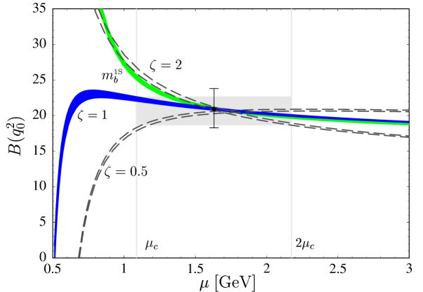
where $\tau_{B}$ is the $B$-meson lifetime. In Figure 2, we show the renormalization-scale dependence of $B(q_{0}^{2})$ for the optimal choice $q_{0}^{2}=(M_{B}-M_{D})^{2}$ and different mass definitions. We scan the parameters $\lambda_{1}$ and $\bar{\mu}$ entering the expression for $\widehat{\Gamma}_{\geq 5}$ in (27) in the ranges $-0.45\,\mbox{GeV}\leq\lambda_{1}\leq-0.15$ GeV and $\mu\leq\bar{\mu}\leq m_{b}$. The sensitivity to the values of these parameters is very small, as indicated by the widths of the bands. The vertical gray lines indicate the “perturbative window” between $\mu=\mu_{c}$ and $2\mu_{c}$ (calculated with $\zeta=1$). In this range there are no large logarithms, and the coupling $\alpha_{s}(\mu)$ is reasonably small. We observe good stability of the results in this region, and an excellent agreement between the PS scheme and the Upsilon scheme for scales above 1.7 GeV. For lower scales, the results in the Upsilon scheme become unstable, whereas the stability interval for the PS scheme extends down to $\mu<1$ GeV. Remarkably, the curves corresponding to the different mass definitions all cross at a point close to the center of the window. We take the central value of the band corresponding to the PS mass with $\zeta=1$, evaluated at the center of the window, as our central value, and use the results obtained with $\zeta=1$, $\mu=\mu_{c}$ and $\zeta=2$, $\mu=2\mu_{c}$ to get an estimate of the perturbative uncertainty.

The error bar at the default point reflects the sensitivity to the value of the $b$-quark mass. The branching ratio scales as approximately the tenth power of $m_{b}$ [8], and because of this strong dependence this is the dominant theoretical uncertainty in our prediction. The dependence on the $b$-quark mass can be parameterized as

$$B(q_{0}^{2})\propto\left(\frac{m_{b}^{\text{PS}}}{4.52\,\mbox{GeV}}\right)^{\Delta(q_{0}^{2})},$$ (32)

where $m_{b}^{\text{PS}}\equiv m_{b}^{\text{PS}}(2\,\mbox{GeV})$, and the exponent $\Delta(q_{0}^{2})$ increases with $q_{0}^{2}$ (see Table 1 below). Alternatively, one may substitute the ratio $m_{b}^{\text{PS}}/4.52$ GeV with $m_{b}^{\text{1S}}/4.72$ GeV or $\overline{m}_{b}(m_{b})/4.20$ GeV. The $\pm 60$ MeV error assumed in the figure is less conservative than the $\pm 80$ MeV advocated in [24], but larger than the $\pm 50$ MeV found in [27].

Table 1: Theoretical predictions for the branching ratio for different values of $q_{0}^{2}$. The optimal choice of the cutoff is $q_{0}^{2}=(M_{B}-M_{D})^{2}\simeq 11.6$ GeV². Errors are added in quadrature and symmetrized in the final result.

$q_{0}^{2}$ [GeV2]	$B(q_{0}^{2})$	$\delta m_{b}$	pert.	$(\Lambda/\mu_{c})^{3}$	$\Delta(q_{0}^{2})$
10.5	$26.9\pm 4.5$	${}_{\,-3.0}^{\,+3.3}$	${}_{\,-3.0}^{\,+2.1}$	$\pm 2.0$	$\phantom{1}8.8$
$(M_{B}-M_{D})^{2}$	$20.9\pm 4.0$	${}_{\,-2.6}^{\,+2.9}$	${}_{\,-2.3}^{\,+1.8}$	$\pm 2.0$	19.9
13.0	$14.8\pm 3.4$	${}_{\,-2.2}^{\,+2.4}$	${}_{\,-1.5}^{\,+1.3}$	$\pm 2.0$	11.7
15.0	$\phantom{2}7.6\pm 2.7$	${}_{\,-1.6}^{\,+1.8}$	${}_{\,-0.5}^{\,+0.7}$	$\pm 2.0$	16.4

Table 1 shows our final theoretical predictions for $B(q_{0}^{2})$ as a function of the cutoff on the dilepton invariant mass. We separately list the errors due to the uncertainty in the $b$-quark mass, the perturbative uncertainty, and higher-order power corrections. Each of the quantities $\widehat{\Gamma}_{n}$ in (16) receives corrections of order $(\Lambda/\mu_{c})^{3}$, whose contributions are essentially unknown. Because of the prefactor $\delta^{3}=(\mu_{c}/m_{b})^{3}$ in this equation, the corresponding contribution to the decay rate is to first order independent of $q_{0}^{2}$ and scales like $(\Lambda/m_{b})^{3}$. Correspondingly we assign an error of $\pm 16\Gamma_{0}\,(\Lambda/m_{b})^{3}\approx 2\,|V_{ub}|^{2}$, where we have used $\Lambda=500$ MeV as a typical hadronic scale. Recently the possibility has been entertained that it might be possible to lower the $q^{2}$ cutoff below the charm threshold, because the contributions from low-lying charm states can be subtracted using experimental data [29]. We have therefore included a result for $q_{0}^{2}=10.5$ GeV² in the table.

The results in Table 1 compare well with the ones obtained in [8], where a value corresponding to $B(q_{0}^{2})=20.0\pm 3.9$ was obtained for $q_{0}^{2}=(M_{B}-M_{D})^{2}$. A new element of the present analysis is the study of different mass definition schemes, which allows us to obtain a more reliable estimate of the perturbative uncertainty. The authors of [7] have calculated the decay rate in the Upsilon scheme using fixed-order perturbation theory at the scale $\mu=m_{b}$. With this choice of scale and scheme we find $B(q_{0}^{2})=17.8$, significantly less than the central value shown in the table. These authors have also included a partial calculation of higher-order corrections (terms of order $\beta_{0}\alpha_{s}^{2}$) and used $m_{b}^{\text{1S}}=M_{\Upsilon(1S)}/2$ for the Upsilon mass (with no uncertainty), thereby neglecting the nonperturbative contribution estimated in [27]. Their result reported in [7] corresponds to $B(q_{0}^{2})=(19.3\pm 0.8\,[\mbox{pert}]\pm 1.7\,[\mbox{power}])$. Since the $\beta_{0}\alpha_{s}^{2}$ terms are related to the choice of scale in the leading-order correction, it is not clear to us why the quoted perturbative error is smaller than the contribution of these terms. More importantly, however, the dominant theoretical uncertainty due to the strong sensitivity to the $b$-quark mass has been neglected in [7].

4 Conclusions

We have presented a calculation of the branching ratio for the inclusive decay $B\to X_{u}\,l\,\nu$ with a cut $q^{2}>q_{0}^{2}\geq(M_{B}-M_{D})^{2}$ on the dilepton invariant mass. Since the typical parton momenta $\sim\mu_{c}$ after the cut are of order the charm-quark mass, we have performed a two-step expansion in the ratios $\mu_{c}/m_{b}$ and $\Lambda/\mu_{c}$ and summed logarithms of the form $\alpha_{s}\ln(\mu_{c}/m_{b})$ at next-to-leading order. To improve the quality of the perturbative result, we have eliminated the pole mass in favor of a low-scale subtracted $b$-quark mass. We find that both the potential subtracted and the Upsilon mass lead to consistent results for the rate. Considering the residual renormalization-scale dependence and the variations between different definitions of the heavy-quark mass, we estimate the perturbative uncertainty to be of order 10%. This is comparable to the size of unknown higher-order power corrections, but smaller than the error arising from the uncertainty on the value of the $b$-quark mass.

If a value of the cutoff not far above the optimal choice $q_{0}^{2}=(M_{B}-M_{D})^{2}$ can be achieved experimentally, we conclude that $|V_{ub}|$ can be determined with a precision of about 10%. This would be considerably less than the current theoretical uncertainty in the value of this important Standard Model parameter.

Acknowledgements: We are grateful to Martin Beneke for helpful discussions. This work was supported in part by the National Science Foundations of the U.S. and Switzerland.

References

- [1] J. Chay, H. Georgi and B. Grinstein, Phys. Lett. B 247 (1990) 399.
-
[2]
I.I. Bigi, N.G. Uraltsev and A.I. Vainshtein, Phys. Lett. B 293 (1992) 430
[hep-ph/9207214], ibid. 297 (1993) 477 (E);
I.I. Bigi, M. Shifman, N.G. Uraltsev and A. Vainshtein, Phys. Rev. Lett. 71 (1993) 496 [hep-ph/9304225];
B. Blok, L. Koyrakh, M. Shifman and A.I. Vainshtein, Phys. Rev. D 49 (1994) 3356 [hep-ph/9307247], ibid. 50 (1994) 3572 (E). - [3] A.V. Manohar and M.B. Wise, Phys. Rev. D 49 (1994) 1310 [hep-ph/9308246].
- [4] T. van Ritbergen, Phys. Lett. B 454 (1999) 353 [hep-ph/9903226].
[5]
M. Neubert, Phys. Rev. D 49 (1994) 3392 [hep-ph/9311325];
Phys. Rev. D 49 (1994) 4623 [hep-ph/9312311];
T. Mannel and M. Neubert, Phys. Rev. D 50 (1994) 2037 [hep-ph/9402288]. - [6] I.I. Bigi, M.A. Shifman, N.G. Uraltsev and A.I. Vainshtein, Int. J. Mod. Phys. A 9 (1994) 2467 [hep-ph/9312359]; Phys. Lett. B 328 (1994) 431 [hep-ph/9402225].
- [7] C.W. Bauer, Z. Ligeti and M. Luke, Phys. Lett. B 479 (2000) 395 [hep-ph/0002161].
- [8] M. Neubert, J. High Ener. Phys. 0007 (2000) 022 [hep-ph/0006068].
- [9] M. Neubert, Phys. Rep. 245 (1994) 259 [hep-ph/9306320].
- [10] X. Ji and M. J. Musolf, Phys. Lett. B 257 (1991) 409.
- [11] D.J. Broadhurst and A.G. Grozin, Phys. Lett. B 267 (1991) 105 [hep-ph/9908362].
- [12] G. Amoros, M. Beneke and M. Neubert, Phys. Lett. B 401 (1997) 81 [hep-ph/9701375].
- [13] A. Czarnecki and A.G. Grozin, Phys. Lett. B 405 (1997) 142 [hep-ph/9701415].
- [14] A.F. Falk and B. Grinstein, Phys. Lett. B 247 (1990) 406.
- [15] M. Neubert, Phys. Rev. D 49 (1994) 1542 [hep-ph/9308369].
- [16] G. Amoros and M. Neubert, Phys. Lett. B 420 (1998) 340 [hep-ph/9711238].
- [17] T. Becher, M. Neubert and A.A. Petrov, Two-loop renormalization of heavy–light currents at order in the heavy-quark expansion, Preprint CLNS 00/1713 [hep-ph/0012183].
- [18] A.F. Falk and M. Neubert, Phys. Rev. D 47 (1993) 2965 [hep-ph/9209268].
- [19] M. Luke and A.V. Manohar, Phys. Lett. B 286 (1992) 348 [hep-ph/9205228].
- [20] F. De Fazio and M. Neubert, J. High Ener. Phys. 9906 (1999) 017 [hep-ph/9905351].
- [21] M. Beneke, Phys. Lett. B 434 (1998) 115 [hep-ph/9804241].
- [22] A.H. Hoang, Z. Ligeti and A.V. Manohar, Phys. Rev. Lett. 82 (1999) 277 [hep-ph/9809423]; Phys. Rev. D 59 (1999) 074017 [hep-ph/9811239].
[23]
I. Bigi, M. Shifman and N. Uraltsev, Ann. Rev. Nucl. Part. Sci. 47 (1997) 591
[hep-ph/9703290];
A. Czarnecki, K. Melnikov and N. Uraltsev, Phys. Rev. Lett. 80 (1998) 3189 [hep-ph/9708372]. - [24] For a review, see: M. Beneke, talk at the 8th International Symposium on Heavy Flavor Physics (Heavy Flavors 8), Southampton, England, 25–29 July 1999 [hep-ph/9911490].
- [25] M. Jezabek and J.H. Kühn, Nucl. Phys. B 314 (1989) 1.
- [26] M. Beneke and A. Signer, Phys. Lett. B 471 (1999) 233 [hep-ph/9906475].
- [27] A. Hoang, Bottom quark mass from Upsilon mesons: Charm mass effects, Preprint CERN-TH-2000-227 [hep-ph/0008102]; Light quark mass effects in bottom quark mass determinations, Preprint CERN-TH-2001-48 [hep-ph/0102292].
- [28] I. Bigi, M. Shifman, N. Uraltsev and A. Vainshtein, Phys. Rev. D 56 (1997) 4017 [hep-ph/9704245].
- [29] C.W. Bauer, Z. Ligeti and M. Luke, On from the dilepton invariant mass spectrum, Preprint UTPT-00-08 [hep-ph/0007054].