Mass Expansions of Screened Perturbation Theory

Abstract

The thermodynamics of massless $\phi^{4}$-theory is studied within screened perturbation theory (SPT). In this method the perturbative expansion is reorganized by adding and subtracting a mass term in the Lagrangian. We analytically calculate the pressure and entropy to three-loop order and the screening mass to two-loop order, expanding in powers of $m/T$. The truncated $m/T$-expansion results are compared with numerical SPT results for the pressure, entropy and screening mass which are accurate to all orders in $m/T$. It is shown that the $m/T$-expansion converges quickly and provides an accurate description of the thermodynamic functions for large values of the coupling constant.

I Introduction

The behavior of finite temperature field theory at intermediate to large coupling is of particular interest due to the upcoming heavy-ion collision experiments at RHIC and LHC. For years the hope has been that due to the asymptotic freedom of QCD that weak-coupling expansion calculations within finite temperature field theory would suffice to describe the experimental data. Along these lines, there has been significant progress in recent years in perturbative calculations within thermal field theory. The pressure in QCD, for example, is now known to order $g^{5}$ [1, 2, 3]. Unfortunately, an analysis of the convergence of this expansion shows that the successive perturbative approximations do not converge for experimentally accessible temperatures. This lack of convergence, while not surprising, needs to be addressed in order to provide systematic methods for calculating quark-gluon plasma observables.

The lack of convergence of the weak-coupling expansion is not restricted to QCD. In fact, even in simple massless scalar field theories similar convergence problems are encountered. This indicates that the problem might be universal. The universality of the problem means that the technique needed might be quite general and since calculations within scalar theories are technically simpler than in full QCD these theories can provide an important testing ground for methods to deal with this problem. Like QCD, the weak-coupling expansion for the pressure of a massless scalar field theory with a $g^{2}\phi^{4}/4!$ interaction, is known to order $g^{5}$ [1, 4, 5]

$${\cal P} = {\cal P}_{\rm ideal}\left[1-{5\over 4}\alpha+{5\sqrt{6}\over 3}\alpha^{3/2}+{15\over 4}\left(\log{\mu\over 2\pi T}+0.40\right)\alpha^{2}\right.$$ (2)

$$\left.-{15\sqrt{6}\over 2}\left(\log{\mu\over 2\pi T}-{2\over 3}\log\alpha-0.72\right)\alpha^{5/2}+{\cal O}(\alpha^{3}\log\alpha)\right]\;,$$

where ${\cal P}_{\rm ideal}=(\pi^{2}/90)T^{4}$ is the pressure of an ideal gas of free massless bosons, $\alpha=g^{2}(\mu)/16\pi^{2}$, and $g(\mu)$ is the $\overline{\rm MS}$ coupling constant at the renormalization scale $\mu$. In Fig. 1, we show the successive perturbative approximations to ${\cal P}/{\cal P}_{\rm ideal}$ as a function of $g(2\pi T)$. Each partial sum is shown as a band obtained by varying $\mu$ from $\pi T$ to $4\pi T$. To express $g(\mu)$ in terms of $g(2\pi T)$, we use the numerical solution to the renormalization group equation $\mu{\partial\over\partial\mu}\alpha=\beta(\alpha)$ with a five-loop beta function [6]:

$$\mu{\partial\over\partial\mu}\alpha=3\alpha^{2}-{17\over 3}\alpha^{3}+32.54\alpha^{4}-271.6\alpha^{5}+2848.6\alpha^{6}\;.$$ (3)

The lack of convergence of the weak-coupling expansion for large coupling is evident in Fig. 1. The band obtained by varying $\mu$ by a factor of two is not necessarily a good measure of the error, but it is certainly a lower bound on the theoretical error. Another indicator of the theoretical error is the deviation between successive approximations. We can infer from Fig. 1 that the error grows rapidly when $g(2\pi T)$ exceeds 1.5.

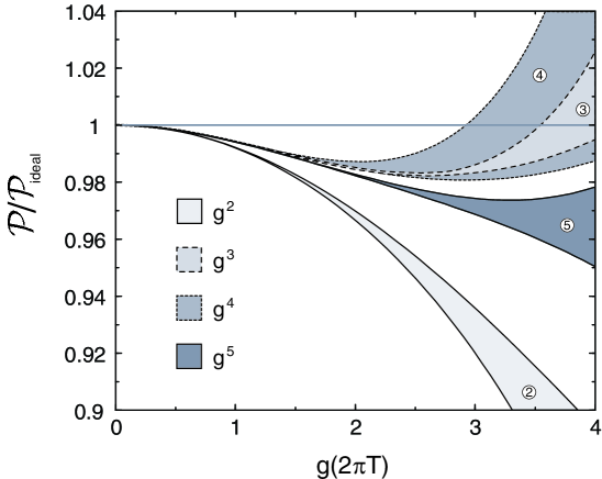
FIG. 1.: Weak-coupling expansion to orders $g^{2}$, $g^{3}$, $g^{4}$, and $g^{5}$ for the pressure normalized to that of an ideal gas as a function of $g(2\pi T)$.

A similar behavior can be seen in the weak-coupling expansion for the screening mass, which has been calculated to order $g^{4}$ [5]. In Fig. 2, we show the screening mass $m_{s}$ normalized to the leading order result $m_{\rm LO}=g(2\pi T)T/\sqrt{24}$ as a function of $g(2\pi T)$, for each of the three successive approximations to $m_{s}^{2}$. The bands correspond to varying $\mu$ from $\pi T$ to $4\pi T$. The poor convergence is again evident. The pattern is similar to that in Fig. 1, with a large deviation between the order-$g^{2}$ and order-$g^{3}$ approximations and a large increase in the size of the band for $g^{4}$.

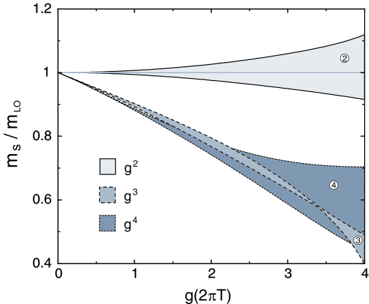
FIG. 2.: Weak-coupling expansion to orders $g^{2}$, $g^{3}$, and $g^{4}$ for the screening mass normalized to the leading-order expression as a function of $g(2\pi T)$.

There are several ways to reorganize perturbation theory to improve its convergence. One method is Padé approximants [7]. This method is limited to observables like the pressure, for which several terms in the weak-coupling expansion are known. Its application is further complicated by the appearance of logarithms of the coupling constant in the coefficients of the weak-coupling expansion. However, the greatest problem with Padé approximants is that, with no understanding of the analytic behavior of ${\cal P}$ at strong coupling, it is little more than a numerological recipe.

An alternative with greater physical motivation is a self-consistent approach [8]. In this method, perturbation theory is reorganized by expressing the free energy as a stationary point of a functional $\Omega$ of the exact self-energy function $\Pi(p_{0},{\bf p})$ called the thermodynamic potential [9]. Since the exact self-energy is not known, $\Pi$ can be regarded as a variational function. The “$\Phi$-derivable” prescription of Baym [8] is to truncate the perturbative expansion for the thermodynamic potential $\Omega$ and to determine $\Pi$ self-consistently as a stationary point of $\Omega$. This gives an integral equation for the self-energy that is hard to solve numerically, unless $\Pi$ is momentum independent. A more tractable approach is to find an approximate solution to the integral equations that is accurate only in the weak-coupling limit. Such an approach has been applied by Blaizot, Iancu, and Rebhan to massless scalar field theories and gauge theories [10, 11].

Another variational approach is screened perturbation theory (SPT) introduced by Karsch, Patkós and Petreczky [12]. This approach is less ambitious than the $\Phi$-derivable approach. Instead of introducing a variational function, it introduces a single variational parameter $m$. This parameter has a simple and obvious physical interpretation as a thermal mass. The advantage of screened perturbation theory is that it is straightforward to apply. Higher order corrections are calculable, so one can test whether it improves the convergence of the weak-coupling expansion. Karsch, Patkós and Petreczky applied screened perturbation theory to a massless scalar field theory with a $\phi^{4}$ interaction, computing the two-loop pressure and the three-loop pressure in the large-$N$ limit.

In Ref. [13], a detailed study of screened perturbation theory for a massless scalar field theory was presented. The pressure and entropy were calculated to three loops and the screening mass to two loops. It was shown that, in contrast to the weak-coupling expansions, the SPT-improved approximations converge even for rather large values of the coupling constant. In Ref. [13], the sum-integrals for the three-loop free energy were evaluated exactly by replacing the sums by contour integrals, extracting the poles in $\epsilon$, and then reducing the momentum integrals to integrals that were at most three-dimensional and could be evaluated numerically. The resulting expressions, while truncated in the coupling constant were “exact” in the sense that they included contributions from all orders in $m/T$. In this paper we continue the study of screened perturbation theory by performing an analytic expansion of the sum-integrals in powers of $m/T$ and demonstrate that the first few terms in the expansion give an accurate approximation to the exact SPT result.

The paper is organized as follows. In section II, we describe the systematics of screened perturbation theory. In section III, we calculate the free energy and entropy to three loops, and the screening mass to two loops, expanding in powers of $m/T$. In Section IV, we calculate the screening mass to two loops using the $m/T$ expansion. In Section V, we briefly discuss the two-loop tadpole gap that generalizes the one-loop gap equation. In Section VI, we study the convergence properties of SPT-improved results for the pressure, entropy, and screening mass using the $m/T$ expansion. Finally, in section VII, we summarize and conclude. Necessary calculational details are collected in four appendices.

II Screened Perturbation Theory

The Lagrangian density for a massless scalar field with a $\phi^{4}$ interaction is

$${\cal L}={1\over 2}\partial_{\mu}\phi\partial^{\mu}\phi-{g^{2}\over 24}\phi^{4}+\Delta{\cal L}\;,$$ (4)

where $g$ is the coupling constant and $\Delta{\cal L}$ includes counterterms. Renormalizability guarantees that $\Delta{\cal L}$ is of the form

$$\Delta{\cal L}={1\over 2}\Delta Z\,\partial_{\mu}\phi\partial^{\mu}\phi-{1\over 24}\Delta g^{2}\phi^{4}\;.$$ (5)

Screened perturbation theory, which was introduced by Karsch, Patkós and Petreczky [12], is simply a reorganization of the perturbation series for thermal field theory. It can be made more systematic by using a framework called “optimized perturbation theory” that Chiku and Hatsuda [14] have applied to a spontaneously broken scalar field theory. The Lagrangian density is written as

$${\cal L}_{\rm SPT}=-{\cal E}_{0}+{1\over 2}\partial_{\mu}\phi\partial^{\mu}\phi-{1\over 2}\left(m^{2}-m_{1}^{2}\right)\phi^{2}-{g^{2}\over 24}\phi^{4}+\Delta{\cal L}+\Delta{\cal L}_{\rm SPT}\;.$$ (6)

Here, ${\cal E}_{0}$ is the vacuum energy density term, and we have added and subtracted mass terms. If we set ${\cal E}_{0}=0$ and $m_{1}^{2}=m^{2}$, we recover the original Lagrangian Eq. (4). Screened perturbation theory is defined by taking $m^{2}$ to be of order unity and $m_{1}^{2}$ to of order $g^{2}$, expanding systematically in powers of $g^{2}$ and setting $m_{1}^{2}=m^{2}$ at the end of the calculation. This defines a reorganization of the perturbative series in which the expansion is about the free field theory defined by

$${\cal L}_{\rm free}=-{\cal E}_{0}+{1\over 2}\partial_{\mu}\phi\partial^{\mu}\phi-{1\over 2}m^{2}\phi^{2}\;.$$ (7)

The interacting term is

$${\cal L}_{\rm int}={1\over 2}m_{1}^{2}\phi^{2}-{g^{2}\over 24}\phi^{4}+\Delta{\cal L}+\Delta{\cal L}_{\rm SPT}\;.$$ (8)

Screened perturbation theory generates new ultraviolet divergences, but they can be cancelled by the additional counterterm in $\Delta{\cal L}_{\rm SPT}$. If we use dimensional regularization and minimal subtraction, the coefficients of these operators are polynomials in $g^{2}$ and $(m^{2}-m_{1}^{2})$. The additional counterterms required to remove the new divergences are

$$\Delta{\cal L}_{\rm SPT}=-\Delta{\cal E}_{0}-{1\over 2}\left(\Delta m^{2}-\Delta m_{1}^{2}\right)\phi^{2}\;.$$ (9)

Several terms in the power series expansions of the counterterms are known from previous calculations at zero temperature. The counterterms $\Delta g^{2}$ and $\Delta m^{2}$ are known to order $\alpha^{5}$ [6]. We will need the coupling constant counterterm only to leading order in $\alpha$:

$$\Delta g^{2}=\left[{3\over 2\epsilon}\alpha+...\right]g^{2}\;.$$ (10)

We need the mass counterterms $\Delta m^{2}$ and $\Delta m^{2}_{1}$ to next-to-leading order and leading order in $\alpha$, respectively:

$$\Delta m^{2} = \left[{1\over 2\epsilon}\alpha+\left({1\over 2\epsilon^{2}}-{5\over 24\epsilon}\right)\alpha^{2}+...\right]m^{2}\;,$$ (11)

$$\Delta m^{2}_{1} = \left[{1\over 2\epsilon}\alpha+...\right]m^{2}_{1}\;.$$ (12)

The counterterm for $\Delta{\cal E}_{0}$ has been calculated to order $\alpha^{4}$ [15]. We will need its expansion only to second order in $\alpha$ and $m_{1}^{2}$:

$$(4\pi)^{2}\Delta{\cal E}_{0} = \left[{1\over 4\epsilon}+{1\over 8\epsilon^{2}}\alpha+\left({5\over 48\epsilon^{3}}-{5\over 72\epsilon^{2}}+{1\over 96\epsilon}\right)\alpha^{2}\right]m^{4}$$ (14)

$$-2\left[{1\over 4\epsilon}+{1\over 8\epsilon^{2}}\alpha\right]m_{1}^{2}m^{2}+{1\over 4\epsilon}m_{1}^{4}\;.$$

III Free energy to three loops

In this section, we calculate the $m/T$ expansions of the pressure and entropy density to three loops in screened perturbation theory. In performing the truncation $m$ is treated as a quantity that is ${\cal O}(g)$ and include all terms which contribute to order $g^{5}$. The diagrams for the free energy that are included at this order are those shown in Fig. 3 together with diagrams involving counterterms.

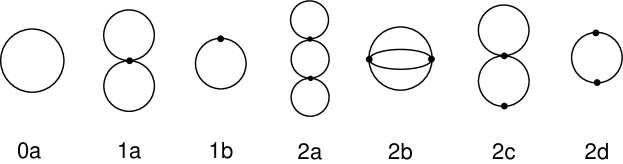
FIG. 3.: Diagrams for the one-loop (0a), two-loop (1a and 1b), and three-loop (2a, 2b, 2c, and 2d) free energy.

A One-loop free energy

The free energy at leading order in $g^{2}$ is

$${\cal F}_{0} = {\cal E}_{0}+{\cal F}_{\rm 0a}+\Delta_{0}{\cal E}_{0}\;,$$ (15)

where $\Delta_{0}{\cal E}_{0}$ is the term of order $g^{0}$ in the vacuum energy counterterm Eq. (14). The expression for diagram 0a in Fig. 3 is

$${\cal F}_{\rm 0a} = {1\over 2}\hbox{$\sum$}\!\!\!\!\!\!\int_{P}\log\left[P^{2}+m^{2}\right]\;,$$ (16)

with $\hbox{$\sum$}\!\!\!\!\!{\displaystyle\int}_{P}$ defined in Appendix A.

Treating $m$ as ${\cal O}(g)$ and including all terms which contribute through ${\cal O}(g^{5})$, we obtain

$${\cal F}_{\rm 0a} = {1\over 2}{\cal I}_{0}^{\prime}+{1\over 2}m^{2}{\cal I}_{1}+{1\over 2}TI_{0}^{\prime}-{1\over 4}m^{4}{\cal I}_{2}+{\cal O}(m^{6}/T^{2})\;,$$ (17)

where ${\cal I}^{\prime}_{0}$ and ${\cal I}_{n}$ are defined in Appendix A and $I^{\prime}_{0}$ is defined in Appendix B.

The resulting expression is logarithmically divergent and the pole in $\epsilon$ is cancelled by the zeroth order term $\Delta_{0}{\cal E}_{0}$ in Eq. (14). The final result for the truncated one-loop free energy is

$${\cal F}_{0} = -{\pi^{2}T^{4}\over 90}\Bigg{[}1-15\hat{m}^{2}+60\hat{m}^{3}+45\hat{m}^{4}(L+\gamma)\Bigg{]}\;,$$ (18)

where $\hat{m}={m\over 2\pi T}$ and $L=\log{\mu\over 4\pi T}$.

B Two-loop free energy

The contribution to the free energy of order $g^{2}$ is

$${\cal F}_{1} = {\cal F}_{\rm 1a}+{\cal F}_{\rm 1b}+\Delta_{1}{\cal E}_{0}+{\partial{\cal F}_{\rm 0a}\over\partial m^{2}}\Delta_{1}m^{2}\;,$$ (19)

where $\Delta_{1}{\cal E}_{0}$ and $\Delta_{1}m^{2}$ are the counterterms of order $g^{2}$, respectively. The expressions for the diagrams 1a and 1b in Fig. 3 are

$${\cal F}_{\rm 1a} = {1\over 8}g^{2}\left(\hbox{$\sum$}\!\!\!\!\!\!\int_{P}{1\over P^{2}+m^{2}}\right)^{2}\;,$$ (20)

$${\cal F}_{\rm 1b} = -{1\over 2}m_{1}^{2}\hbox{$\sum$}\!\!\!\!\!\!\int_{P}{1\over P^{2}+m^{2}}\;.$$ (21)

The sum-integrals in Eqs. (20) and (21) are expanded to the order required:

$${\cal F}_{\rm 1a} = {1\over 8}g^{2}\Bigg{[}{\cal I}_{1}^{2}+2T{\cal I}_{1}I_{1}-2m^{2}{\cal I}_{1}{\cal I}_{2}+T^{2}I_{1}^{2}-2m^{2}T{\cal I}_{2}I_{1}\Bigg{]}\;,$$ (22)

$${\cal F}_{\rm 1b} = -{1\over 2}m_{1}^{2}\Bigg{[}{\cal I}_{1}+TI_{1}-m^{2}{\cal I}_{2}\Bigg{]}\;,$$ (23)

where $I_{n}$ is defined in Appendix B.

The poles in $\epsilon$ in Eqs. (22) and (23) are cancelled by the counterterms in Eq. (19). The final result for the truncated two-loop free energy is

$${\cal F}_{1} = {g^{2}T^{4}\over 1152}\Bigg{[}1-12\hat{m}-12\hat{m}^{2}\left(L+\gamma-3\right)+72(L+\gamma)\hat{m}^{3}\Bigg{]}$$ (25)

$$-{m_{1}^{2}T^{2}\over 24}\Bigg{[}1-6\hat{m}-6\hat{m}^{2}(L+\gamma)\Bigg{]}\;.$$

C Three-loop free energy

The contribution to the free energy of order $g^{4}$ is

$${\cal F}_{2} = {\cal F}_{\rm 2a}+{\cal F}_{\rm 2b}+{\cal F}_{\rm 2c}+{\cal F}_{\rm 2d}+\Delta_{2}{\cal E}_{0}+{\partial{\cal F}_{\rm 0a}\over\partial m^{2}}\Delta_{2}m^{2}+{1\over 2}{\partial^{2}{\cal F}_{\rm 0a}\over\left(\partial m^{2}\right)^{2}}\left(\Delta_{1}m^{2}\right)^{2}$$ (27)

$$+\left({\partial{\cal F}_{\rm 1a}\over\partial m^{2}}+{\partial{\cal F}_{\rm 1b}\over\partial m^{2}}\right)\Delta_{1}m^{2}+{{\cal F}_{\rm 1a}\over g^{2}}\Delta_{1}g^{2}+{{\cal F}_{\rm 1b}\over m_{1}^{2}}\Delta_{1}m_{1}^{2}\;,$$

where we have included all necessary counterterms. The expressions for the diagrams $2a$, $2b$, $2c$, and $2d$ in Fig. 3 are

$${\cal F}_{\rm 2a} = -{1\over 16}g^{4}\left(\hbox{$\sum$}\!\!\!\!\!\!\int_{P}{1\over P^{2}+m^{2}}\right)^{2}\hbox{$\sum$}\!\!\!\!\!\!\int_{Q}{1\over(Q^{2}+m^{2})^{2}}\;,$$ (28)

$${\cal F}_{\rm 2b} = -{1\over 48}g^{4}\hbox{$\sum$}\!\!\!\!\!\!\int_{PQR}{1\over P^{2}+m^{2}}{1\over Q^{2}+m^{2}}{1\over R^{2}+m^{2}}{1\over(P+Q+R)^{2}+m^{2}}\;,$$ (29)

$${\cal F}_{\rm 2c} = {1\over 4}g^{2}m_{1}^{2}\hbox{$\sum$}\!\!\!\!\!\!\int_{P}{1\over P^{2}+m^{2}}\hbox{$\sum$}\!\!\!\!\!\!\int_{Q}{1\over(Q^{2}+m^{2})^{2}}\;,$$ (30)

$${\cal F}_{\rm 2d} = -{1\over 4}m_{1}^{4}\hbox{$\sum$}\!\!\!\!\!\!\int_{P}{1\over(P^{2}+m^{2})^{2}}\;.$$ (31)

Expanding in powers of $m^{2}$ to the appropriate order gives

$${\cal F}_{\rm 2a} = -{1\over 16}g^{4}\Bigg{[}T{\cal I}_{1}^{2}I_{2}+{\cal I}_{1}^{2}{\cal I}_{2}+2T^{2}{\cal I}_{1}I_{1}I_{2}+T^{3}I_{1}^{2}I_{2}+2TI_{1}{\cal I}_{1}{\cal I}_{2}-2m^{2}T{\cal I}_{1}{\cal I}_{2}I_{2}\Bigg{]}\;,$$ (32)

$${\cal F}_{\rm 2b} = -{1\over 48}g^{4}\Bigg{[}{\cal I}_{\rm ball}+T^{3}I_{\rm ball}+4TI_{1}{\cal I}_{\rm sun}(0)\Bigg{]}\;,$$ (33)

$${\cal F}_{\rm 2c} = {1\over 4}g^{2}m_{1}^{2}\Bigg{[}T{\cal I}_{1}I_{2}+{\cal I}_{1}{\cal I}_{2}+T^{2}I_{1}I_{2}+T{\cal I}_{2}I_{1}-m^{2}T{\cal I}_{2}I_{2}\Bigg{]}\;,$$ (34)

$${\cal F}_{\rm 2d} = -{1\over 4}m_{1}^{4}\Bigg{[}{\cal I}_{2}+TI_{2}\Bigg{]}\;,$$ (35)

where $I_{\rm ball}$, ${\cal I}_{\rm sun}$, and ${\cal I}_{\rm ball}$ are defined in Appendices B, C, D respectively.

The poles in $\epsilon$ in Eqs. (32)-(35) are cancelled by the counterterms in Eq. (27). The final result for the truncated three-loop free energy is

$${\cal F}_{2} = -{g^{4}T^{4}\over 2304(4\pi)^{2}\hat{m}}\Bigg{[}1-2\hat{m}\Bigg{(}{59\over 15}-\gamma-3L+2{\zeta^{\prime}(-3)\over\zeta(-3)}-4{\zeta^{\prime}(-1)\over\zeta(-1)}\Bigg{)}$$ (39)

$$\hskip 14.22636pt-12\hat{m}^{2}\Bigg{(}5+7L+3\gamma-8\log\hat{m}-8\log 2-4{\zeta^{\prime}(-1)\over\zeta(-1)}\Bigg{)}\Bigg{]}$$

$$\hskip 14.22636pt+{g^{2}m_{1}^{2}T^{2}\over 48(4\pi)^{2}\hat{m}}\Bigg{[}1+2\hat{m}\left(L+\gamma-3\right)-18\hat{m}^{2}(L+\gamma)\Bigg{]}$$

$$\hskip 14.22636pt-{m_{1}^{4}\over 64\hat{m}}\Bigg{[}1+2\hat{m}(L+\gamma)\Bigg{]}\;.$$

D Pressure to three loops

The pressure ${\cal P}$ is given by $-{\cal F}$. The contributions to the pressure of zeroth, first, and second order in $g^{2}$ are given by Eqs. (18), (25), and (39), respectively. Adding these contributions and setting ${\cal E}_{0}=0$ and $m_{1}^{2}=m^{2}$, we obtain approximations to the pressure in screened perturbation theory which are accurate to ${\cal O}(g^{5})$.

The one-loop approximation to the pressure is

$${\cal P}_{0} = {\cal P}_{\rm ideal}\Bigg{[}1-15\hat{m}^{2}+60\hat{m}^{3}+45\hat{m}^{4}(L+\gamma)\Bigg{]}\;.$$ (40)

The two-loop approximation to the pressure is obtained by adding Eq. (25) with $m_{1}^{2}=m^{2}$:

$${\cal P}_{0+1} = {\cal P}_{\rm ideal}\Bigg{\{}1-{5\over 4}\alpha+15\hat{m}\alpha+15\hat{m}^{2}(L+\gamma-3)\alpha$$ (42)

$$\hskip 56.9055pt-30\hat{m}^{3}\bigg{[}1+3(L+\gamma)\alpha\bigg{]}-45\hat{m}^{4}(L+\gamma)\Bigg{\}}\;.$$

The three-loop approximation to the pressure is obtained by adding Eq. (39) with $m_{1}^{2}=m^{2}$:

$${\cal P}_{0+1+2} = {\cal P}_{\rm ideal}\Bigg{\{}1-{5\over 4}\alpha+\Bigg{[}-{59\over 12}+{15\over 4}L+{5\over 4}\gamma-{5\over 2}{\zeta^{\prime}(-3)\over\zeta(-3)}+5{\zeta^{\prime}(-1)\over\zeta(-1)}\Bigg{]}\alpha^{2}$$ (45)

$$\hskip 14.22636pt+{15\over 2}\hat{m}\Bigg{[}1-\Bigg{(}5+3\gamma+7L-8\log\hat{m}-8\log 2-4{\zeta^{\prime}(-1)\over\zeta(-1)}\Bigg{)}\alpha\Bigg{]}\alpha$$

$$\hskip 28.45274pt-{15\over 2}\hat{m}^{3}\Bigg{[}1-6(L+\gamma)\alpha\Bigg{]}+{5\over 8\hat{m}}\alpha^{2}\Bigg{\}}\;.$$

Note that if we substitute the leading-order result for the screening mass, $m=g(2\pi T)T/\sqrt{24}$, in Eq. (45), we recover the weak-coupling expansion through order $g^{5}$.

E Entropy to three loops

Given a diagrammatic expansion for the free energy ${\cal F}$, the entropy density ${\cal S}$ has a diagrammatic expansion defined by

$$S_{\rm diag} = -{\!\!\partial\over\partial T}{\cal F}(T,g,m,m_{1},\mu)\;,$$ (46)

where the partial derivative is taken with all the other variables $g$, $m$, $m_{1}$, and $\mu$ held fixed. The one-, two-, and three-loop approximations to ${\cal S}$ are then obtained by taking partial derivatives of the corresponding expressions for the pressure ${\cal P}$.

The one-loop approximation to the entropy ${\cal S}$ is obtained by differentiating Eq.(40)

$${\cal S}_{0} = {\cal S}_{\rm ideal}\Bigg{[}1-{15\over 2}\hat{m}^{2}+15\hat{m}^{3}-{45\over 4}\hat{m}^{4}\Bigg{]}\;,$$ (47)

where ${\cal S}_{\rm ideal}=(2\pi^{2}/45)T^{3}$.

The two-loop approximation to the the entropy ${\cal S}$ is obtained by differentiating Eq.(42)

$${\cal S}_{0+1} = {\cal S}_{\rm ideal}\Bigg{\{}1-{5\over 4}\alpha+{45\over 4}\hat{m}\alpha+{15\over 2}\hat{m}^{2}\left(L+\gamma-{7\over 2}\right)\alpha$$ (49)

$$\hskip 56.9055pt-{15\over 2}\hat{m}^{3}\bigg{[}1+3\left(L+\gamma-1\right)\alpha\bigg{]}+{45\over 4}\hat{m}^{4}\Bigg{\}}\;.$$

The three-loop approximation to the the entropy ${\cal S}$ is obtained by differentiating Eq.(45)

$${\cal S}_{0+1+2} = {\cal S}_{\rm ideal}\Bigg{\{}1-{5\over 4}\alpha+\Bigg{(}-{281\over 48}+{5\over 4}\gamma+{15\over 4}L+5{\zeta^{\prime}(-1)\over\zeta(-1)}-{5\over 2}{\zeta^{\prime}(-3)\over\zeta(-3)}\Bigg{)}\alpha^{2}$$ (52)

$$\hskip 14.22636pt+{45\over 8}\hat{m}\Bigg{[}1-\Bigg{(}{16\over 3}+7L+3\gamma-8\log\hat{m}-4{\zeta^{\prime}(-1)\over\zeta(-1)}-8\log 2\Bigg{)}\alpha\Bigg{]}\alpha$$

$$\hskip 28.45274pt-{15\over 8}\hat{m}^{3}\Bigg{[}1-6(L+\gamma-1)\alpha\Bigg{]}+{25\over 32\hat{m}}\alpha^{2}\Bigg{\}}\;.$$

IV Screening mass to two loops

In this section, we calculate the $m/T$ expansion of the screening mass to two loops. The diagrams for the self energy that are included at this order are those shown in Fig. 4 together with diagrams involving counterterms.

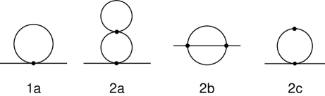
FIG. 4.: Diagrams for the one-loop (1a and 1b) and two-loop (2a, 2b and 2c) self-energy.

The screening mass $m_{s}$ is defined by the location of the pole of the static propagator:

$${\bf p}^{2}+m^{2}+\Pi(0,{\bf p})=0\hskip 56.9055pt\mbox{at}\hskip 28.45274pt{\bf p}^{2}=-m^{2}_{s}\;,$$ (53)

where $\Pi(p_{0},{\bf p})$ is the self-energy function. This equation can be solved order-by-order in powers of $\alpha$ and $m_{1}^{2}$. The solution at zeroth order in $g^{2}$ is simply $m_{s}^{2}=m^{2}$.

A One-loop self-energy

The self-energy to leading order in $g^{2}$ is

$$\Pi_{1}=\Pi_{\rm 1a}-m_{1}^{2}+\Delta_{1}m^{2}\;,$$ (54)

where $\Delta_{1}m^{2}$ is the mass counterterm of order $\alpha$ given in Eq. (11). The expression for the diagram 1a in Fig. 4 is

$$\Pi_{\rm 1a} = {1\over 2}g^{2}\hbox{$\sum$}\!\!\!\!\!\!\int_{P}{1\over P^{2}+m^{2}}\;.$$ (55)

This diagram is expanded to second order in $m^{2}$:

$$\Pi_{\rm 1a} = {1\over 2}g^{2}\Bigg{[}{\cal I}_{1}+TI_{1}-m^{2}{\cal I}_{2}\Bigg{]}\;.$$ (56)

The pole in Eq. (56) is cancelled by the counterterm $\Delta_{1}m^{2}$. The final result for the one-loop self-energy is

$$\Pi_{\rm 1}={g^{2}T^{2}\over 24}\Bigg{[}1-6\hat{m}-6\hat{m}^{2}\left(L+\gamma\right)\Bigg{]}-m_{1}^{2}\;.$$ (57)

B Two-loop self-energy

The contribution to the self-energy of second order in $g^{2}$ is

$$\Pi_{2}(P)=\Pi_{\rm 2a}+\Pi_{\rm 2b}(P)+\Pi_{\rm 2c}+{\partial\Pi_{\rm 1a}\over\partial m^{2}}\Delta_{1}m^{2}+{\Pi_{\rm 1a}\over g^{2}}\Delta_{1}g^{2}+\Delta_{2}m^{2}-\Delta_{1}m_{1}^{2}\;.$$ (58)

The expressions for the diagrams 2a, 2b, and 2c in Fig. 4 are

$$\Pi_{\rm 2a} = -{1\over 4}g^{4}\hbox{$\sum$}\!\!\!\!\!\!\int_{Q}{1\over Q^{2}+m^{2}}\hbox{$\sum$}\!\!\!\!\!\!\int_{R}{1\over(R^{2}+m^{2})^{2}}\;,$$ (59)

$$\Pi_{\rm 2b}(P) = -{1\over 6}g^{4}\hbox{$\sum$}\!\!\!\!\!\!\int_{QR}{1\over Q^{2}+m^{2}}{1\over R^{2}+m^{2}}{1\over(P+Q+R)^{2}+m^{2}}\;,$$ (60)

$$\Pi_{\rm 2c} = {1\over 2}g^{2}m_{1}^{2}\hbox{$\sum$}\!\!\!\!\!\!\int_{Q}{1\over(Q^{2}+m^{2})^{2}}\;.$$ (61)

The diagrams $\Pi_{\rm 2a}$ and $\Pi_{\rm 2c}$ are independent of the momentum $P$. Expanding to first order in $m^{2}$, we obtain

$$\Pi_{\rm 2a} = -{1\over 4}g^{4}\Bigg{[}T{\cal I}_{1}I_{2}+{\cal I}_{1}{\cal I}_{2}+T^{2}I_{1}I_{2}\Bigg{]}\;.$$ (62)

$$\Pi_{\rm 2c} = {1\over 2}g^{2}m_{1}^{2}\Bigg{[}{\cal I}_{2}+TI_{2}\Bigg{]}$$ (63)

The diagram $\Pi_{\rm 2b}$ depends on the external momentum $P$. The equation (53) for the screening mass involves the self-energy at $p_{0}=0$. To calculate the screening mass to second order in $g^{2}$, we need the analytic continuation of $\Pi(0,{\bf p})$ to ${\bf p}^{2}=-m^{2}$. The diagram is calculated in Appendix C. The result is

$$\Pi_{\rm 2b}(0,{\bf p})\Bigg{|}_{{\bf p}^{2}=-m^{2}} = -{1\over 6}g^{4}\Bigg{[}{\cal I}_{\rm sun}(0)+I_{\rm sun}\Bigg{]}\;,$$ (64)

where $I_{\rm sun}$ is defined in Appendix B.

The poles in Eqs. (62)-(64) are cancelled by the counterterms in Eq. (58). The final result for the truncated two-loop contribution to the self-energy at $p_{0}=0$ and ${\bf p}^{2}=-m^{2}$ is

$$\Pi_{2}(0,{\bf p})\Bigg{|}_{{\bf p}^{2}=-m^{2}} = -{g^{4}T^{2}\over 768\pi^{2}\hat{m}}\Bigg{\{}1+2\hat{m}\left[3L+\gamma+1-4\log\hat{m}-8\log 2-2{\zeta^{\prime}(-1)\over\zeta(-1)}\right]\Bigg{\}}$$ (66)

$$\hskip 56.9055pt+{g^{2}m_{1}^{2}\over 32\pi^{2}\hat{m}}\Bigg{[}1+2\left(L+\gamma\right)\hat{m}\Bigg{]}\;.$$

C Screening mass

Since the dependence of the self-energy on the momentum enters only at order $g^{4}$ and since the leading-order solution to the screening mass is $m_{s}=m$, the solution to the equation (53) to order $g^{4}$ is simply

$$m_{s}^{2}=m^{2}+\Pi(0,{\bf p}^{2})\Bigg{|}_{{\bf p}^{2}=-m^{2}}\;.$$ (67)

The result for the one-loop screening mass is

$$\hat{m}_{s}^{2}={1\over 6}\alpha\Bigg{[}1-6\hat{m}-6\hat{m}^{2}\left(L+\gamma\right)\Bigg{]}\;.$$ (68)

The solution to order $g^{4}$ is obtained by inserting the sum of Eqs. (57) and (66) into Eq (67). Setting $m_{1}^{2}=m^{2}$, the result is

$$\hat{m}_{s}^{2} = {1\over 6}\alpha\Bigg{\{}1-{1\over 2\hat{m}}\alpha-\left[3L+\gamma+1+4\log\hat{m}-8\log 2-2{\zeta^{\prime}(-1)\over\zeta(-1)}\right]\alpha-3\hat{m}\Bigg{\}}\;.$$ (69)

If we substitute the leading-order result for the screening mass, $m=g(2\pi T)T/\sqrt{24}$, in Eq. (69), we recover the weak-coupling expansion through order $g^{4}$ [5].

V Gap Equation

The mass parameter $m$ in screened perturbation theory is completely arbitrary. To complete the calculation it is necessary to specify $m$ as a function of $g$ and $T$. One of the complications from the ultraviolet divergences is that the parameters ${\cal E}_{0}$, $m^{2}$, $g^{2}$, and $m_{1}^{2}$ all become running parameters that depend on a renormalization scale $\mu$. In our prescription for recovering the original theory, we must therefore specify the renormalization scale $\mu_{*}$ at which the Lagrangian (6) reduces to Eq. (4). The prescription can be written

$${\cal E}_{0}(\mu_{*}) =0 \,,$$ (70)

$$m^{2}(\mu_{*}) = m_{1}^{2}(\mu_{*})=m^{2}_{*}(T),$$ (71)

where $m_{*}(T)$ is some prescribed function of the temperature.

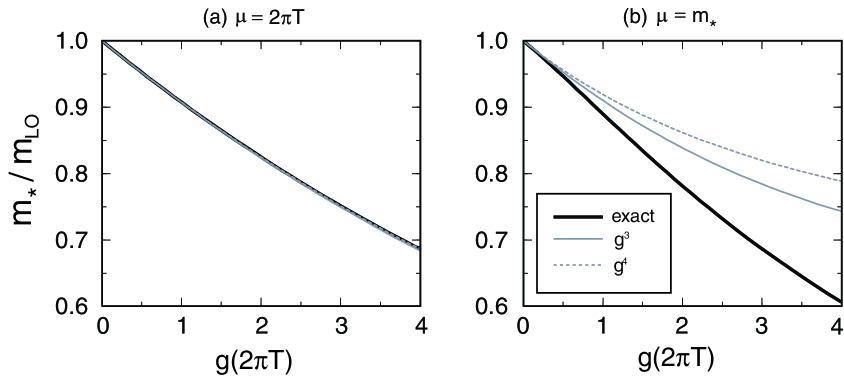
FIG. 5.: Solutions $m_{*}(T)$ to the one-loop tadpole gap equation as a function of $g(2\pi T)$ for (a) $\mu=2\pi T$ and (b) $\mu=m_{*}$. Exact SPT curves are taken from Ref. [13].

The prescription of Karsch, Patkós, and Petreczky for $m_{*}(T)$ is the solution to the one-loop gap equation:

$$m_{*}^{2}={1\over 2}\alpha(\mu_{*})\left[J_{1}(m_{*}/T)T^{2}-\left(2\log{\mu_{*}\over m_{*}}+1\right)m_{*}^{2}\right]\;.$$ (72)

Their choice for the scale was $\mu_{*}=T$. The function $J_{1}(\beta m)$ is defined as

$$J_{1}(\beta m) = 8\beta^{2}\int_{0}^{\infty}dk\;{k^{2}\over\left(k^{2}+m^{2}\right)^{1/2}}{1\over e^{\beta\left(k^{2}+m^{2}\right)^{1/2}}-1}\;.$$ (73)

In the limit $\beta m\longrightarrow 0$, this integral reduces to

$$J_{1}(\beta m) \longrightarrow {4\pi^{2}\over 3}\;-\;4\pi\beta m\;-\;2\left(\log{\beta m\over 4\pi}-{1\over 2}+\gamma\right)(\beta m)^{2}\;.$$ (74)

In the same limit, Eq. (72) reduces to

$$\hat{m}_{*}^{2}={1\over 6}\alpha\Bigg{[}1-6\hat{m}_{*}-6\hat{m}^{2}_{*}\left(L+\gamma\right)\Bigg{]}\;.$$ (75)

The one-loop gap equation is identical to the one-loop screening mass if we choose $m=m_{s}=m_{*}$

Various mass prescriptions that generalize Eq. (72) were extensively studied in Ref. [13]. In this paper, we confine ourselves to using the tadpole mass which is defined by $m_{t}^{2}={1\over 2}g^{2}\langle\phi^{2}\rangle$. This can also be expressed as a derivative of the free energy:

$$m_{t}^{2}=g^{2}{\!\!\!\!\!\!\partial\over\partial m^{2}}{\cal F}(T,g,m,m_{1},\mu)\Bigg{|}_{m_{1}=m}\;,$$ (76)

where the partial derivative is taken before setting $m_{1}=m$.

The one-loop expression for the tadpole mass is given differentiating Eq. (18):

$$\hat{m}_{t}^{2}={1\over 6}\alpha\Bigg{[}1-6\hat{m}-6\hat{m}^{2}\left(L+\gamma\right)\Bigg{]}\;.$$ (77)

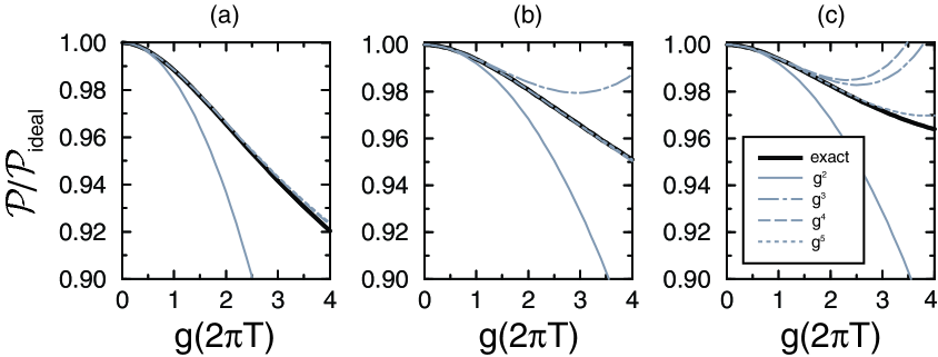
FIG. 6.: The one-, two and three-loop SPT improved approximations to the pressure as a function of $g(2\pi T)$ for $\mu=2\pi T$. Exact SPT curves are taken from Ref. [13].

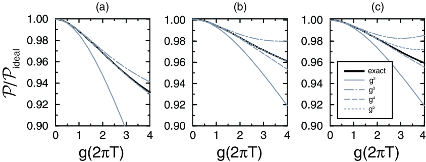
FIG. 7.: The one-, two and three-loop SPT improved approximations to the pressure as a function of $g(2\pi T)$ for $\mu=m_{*}$. Exact SPT curves are taken from Ref. [13].

In Fig. 5, we show the truncated solutions $m_{*}(T)$ to the one-loop tadpole gap equation as a function of $g(2\pi T)$ for (a) $\mu=2\pi T$ and (b) $\mu=m_{*}$. The solutions have been normalized to the leading order screening mass $m_{\rm LO}=g(2\pi T)T/\sqrt{24}$. The truncated solutions were determined by treating $m$ as a quantity that is ${\cal O}(g)$ and truncating at a fixed order in $g$. A $g^{2}$ truncation of Eq. (75), for example, yields $\hat{m}_{*}^{2}=\alpha/6$, which corresponds to the leading order screening mass. The non-trivial truncations, $g^{3}$ and $g^{4}$, are shown as grey dashed lines along with “exact” curves from Ref. [13] which are accurate to all orders in $m/T$. As can been seen from the figure, the gap equation converges very quickly to the exact solutions for $\mu=2\pi T$ while for $\mu=m_{*}$ they do not seem to be converging. The primary difference between the two scales is that in the case $\mu=m_{*}$ there are additional $\log\hat{m}$. It is possible that these logs need to be further resummed. Note that as the renormalized coupling constant becomes larger than $g(2\pi T)\sim 4$ the uncertainty due to the variation of the renormalization scale $\mu$ becomes rather large due to the Landau singlarity present in the running of $g$. For this reason, in all results presented, we restrict ourselves to $g(2\pi T)\leq 4$.

VI SPT-improved variables

In this section, we use the solutions to the tadpole gap equation obtained in Sec. V to obtain successive approximations to the pressure, screening mass, and entropy in screened perturbation theory.

A Pressure

The two-loop SPT-improved approximation to the pressure is obtained by inserting the solution to the one-loop gap equation (72) into the two-loop pressure (42). We can simplify the expression by using Eq. (72) to eliminate the explicit appearance of logarithms of $\mu$. This eliminates all the terms of order $\alpha$ and the expression reduces to

$${\cal P}_{0+1} = {\cal P}_{\rm ideal}\Bigg{[}1-{15\over 2}\hat{m}^{2}+15\hat{m}^{3}\Bigg{]}\;.$$ (78)

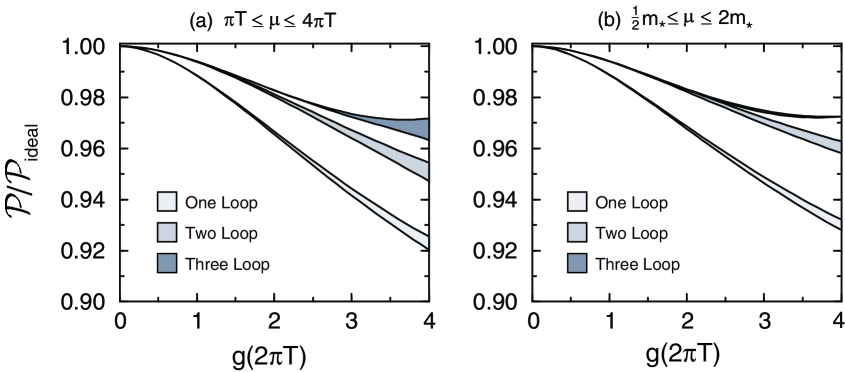
FIG. 8.: The one-, two and three-loop SPT improved approximations to the pressure as a function of $g(2\pi T)$ for (a) $\pi T<\mu<4\pi T$ and (b) ${1\over 2}m_{*}<\mu<2m_{*}$.

In Figs. 6 and 7, we show truncations of the one-, two-, and three-loop approximations to the pressure for $\mu=2\pi T$ and $\mu=m_{*}$, respectively. The various truncations are shown as grey dashed lines along with “exact” curves from Ref. [13] which are accurate to all orders in $m/T$. As can be seen from the figure, the $m/T$ truncations converge very quickly for the one- and two-loop approximations with the final two truncations being virtually indistinguishable from the exact SPT solutions. At three-loops, however, one needs to include all terms up to $g^{5}$ before a reasonable approximation is obtained. We therefore conclude that it is necessary to include higher order terms in order to fully converge to the exact SPT result at three-loops. Also it appears that the $m/T$ truncations converge better for $\mu=2\pi T$, than for $\mu=m_{*}$. Despite these caveats, at all loop orders presented here, the highest order $m/T$ truncation provide an excellent approximation to the exact SPT results.

In Fig. 8 we show the one-, two-, and three-loop approximations obtained using our $g^{5}$ truncation to the pressure. The bands shown correspond to the results obtained by varying the renormalization scale $\mu$ over (a) $\pi T<\mu<4\pi T$ and (b) ${1\over 2}m_{*}<\mu<2m_{*}$. This figure demonstrates that the $g^{5}$ truncations of the pressure yield a convergent series of approximations which have very small variations with respect to the renormalization scale.

B Screening Mass

The one-loop SPT-improved approximation to the screening mass $m_{s}$ is given by the solution to the tadpole gap equation (76). A two-loop SPT-improved approximation can be obtained by inserting the solution to the gap equation for the mass parameter into Eq. (69).

In Fig. 9, we show the $g^{4}$ truncations of the one- and two-loop approximations to the screening mass. The bands shown correspond to the results obtained by varying the renormalization scale $\mu$ over (a) $\pi T<\mu<4\pi T$ and (b) ${1\over 2}m_{*}<\mu<2m_{*}$. One can see from this figure that the convergence of the $m/T$ expansion for the screening mass is not as impressive as for the pressure meaning that higher order truncations are necessary to reliably describe the screening mass. Also, we again see that the $m/T$ truncations converge better for $\mu=2\pi T$, than for $\mu=m_{*}$.

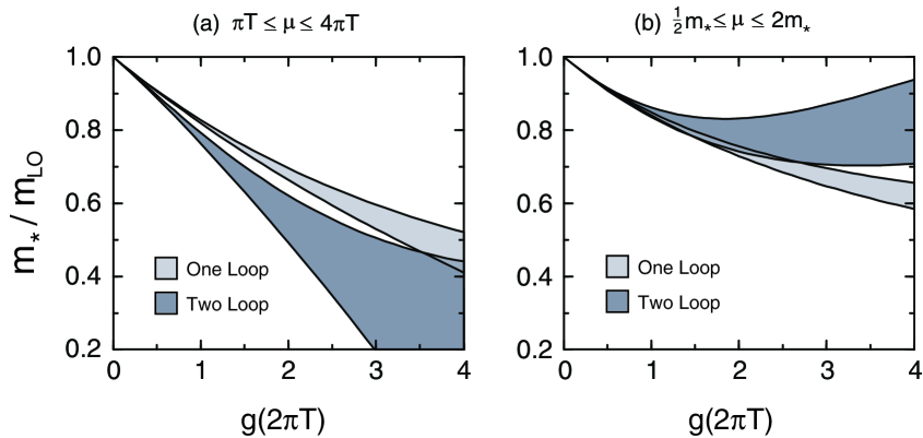
FIG. 9.: The one- and two-loop SPT improved approximations to the screening mass as a function of $g(2\pi T)$ (a) $\pi T<\mu<4\pi T$ and (b) ${1\over 2}m_{*}<\mu<2m_{*}$.

C Entropy

The one, two-, and three-loop SPT-improved entropies are obtained by replacing $m$ in the expressions (47)-(52) for ${\cal S}_{0}$, ${\cal S}_{0+1}$, and ${\cal S}_{0+1+2}$ with the solution to the one-loop gap equation. As was the case with the two-loop pressure we can use the gap equation to eliminate the logarithm $L$ yielding the following expression for the two-loop entropy

$${\cal S}_{0+1}={\cal S}_{\rm ideal}\Bigg{[}1-{15\over 2}\hat{m}^{2}T+15\hat{m}^{3}-{45\over 4}\hat{m}^{4}\Bigg{]}\;.$$ (79)

This is identical to the one-loop expression Eq. (47), which is the entropy of an ideal gas of particles with mass $m$.

In Fig. 10, we show the ${\cal O}(g^{5})$ truncations of the one-, two-, and three-loop approximations to the entropy as a function of $g(2\pi T)$. The bands shown correspond to the results obtained by varying the renormalization scale $\mu$ over (a) $\pi T<\mu<4\pi T$ and (b) ${1\over 2}m_{*}<\mu<2m_{*}$. In both cases the ${\cal O}(g^{5})$ truncation provides an excellent approximation to the exact SPT result. Again we see that the $m/T$ truncations converge better for $\mu=2\pi T$, than for $\mu=m_{*}$.

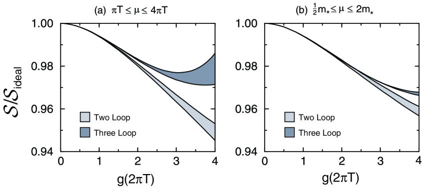
FIG. 10.: The SPT-improved two- and three-loop approximations to the entropy as a function of $g(2\pi T)$ (a) $\pi T<\mu<4\pi T$ and (b) ${1\over 2}m_{*}<\mu<2m_{*}$.

VII Conclusions

In this paper, we have continued the systematic study of screened perturbation theory from Ref. [13]. We applied it to the pressure and the entropy calculated to three loops and the screening mass calculated to two loops. By performing an expansion of the sum-integrals in powers of $m/T$, we were able to obtain purely analytical results, without having to evaluate integrals numerically.

Our calculations show that a truncation of the $m/T$ expansion at ${\cal O}(g^{5})$ is sufficient to obtain accurate approximations to the exact one- and two-loop results. For the one- and two-loop approximations to the pressure and entropy, the numerical results obtained in [13] and the truncated $m/T$ expansions are virtually indistinguishable as can be seen in Figs. 6 and 7. At three-loop the ${\cal O}(g^{5})$ truncation provides a reasonable description of the pressure, but it seems that higher-order truncations are necessary to provide accurate descriptions. The fact that the $m/T$ expansions converge quickly is important since performing the “exact” SPT calculations is much more difficult than the $m/T$ expansions. An additional benefit of the $m/T$ expansion method is that the final results can be determined completely analytically.

In Ref. [16], a generalization of SPT to gauge theories based on hard thermal loop (HTL) perturbation theory was proposed. The thermodynamic functions such as the pressure and entropy were calculated to one-loop order. The two-loop calculation of the pressure in QCD based on HTL perturbation theory requires not only HTL propagators, but HTL vertices as well. The exact calculation appears to be very difficult. Expansions like the one presented here provide the simplification needed to complete the two-loop HTL calculation [17]. The rapid convergence of the $m/T$ expansion in screened perturbation theory is very encouraging in this regard.

A Sum-integrals

In the imaginary-time formalism for thermal field theory, the 4-momentum $P=(P_{0},{\bf p})$ is Euclidean with $P^{2}=P_{0}^{2}+{\bf p}^{2}$. The Euclidean energy $p_{0}$ has discrete values: $P_{0}=2n\pi T$ for bosons and $P_{0}=(2n+1)\pi T$ for fermions, where $n$ is an integer. Loop diagrams involve sums over $P_{0}$ and integrals over ${\bf p}$. With dimensional regularization, the integral is generalized to $d=3-2\epsilon$ spatial dimensions. We define the dimensionally regularized sum-integral by

$$\hbox{$\sum$}\!\!\!\!\!\!\int_{P} \;\equiv\; \left(\frac{e^{\gamma}\mu^{2}}{4\pi}\right)^{\epsilon}\;T\sum_{P_{0}=2n\pi T}\>\int{d^{3-2\epsilon}p\over(2\pi)^{3-2\epsilon}}\;,$$ (A.1)

where $3-2\epsilon$ is the dimension of space and $\mu$ is an arbitrary momentum scale. The factor $(e^{\gamma}/4\pi)^{\epsilon}$ is introduced so that, after minimal subtraction of the poles in $\epsilon$ due to ultraviolet divergences, $\mu$ coincides with the renormalization scale of the $\overline{\rm MS}$ renormalization scheme.

The one-loop sum-integrals that arise in the calculations have the following form

$${\cal I}^{\prime}_{0} = \hbox{$\sum$}\!\!\!\!\!\!\int_{P}\log P^{2}\;,$$ (A.2)

$${\cal I}_{n} = \hbox{$\sum$}\!\!\!\!\!\!\int_{P}{1\over(P^{2})^{n}}\;.$$ (A.3)

Expanding in $\epsilon$ to the required order, the specific one-loop sum-integrals needed are

$${\cal I}_{0}^{\prime} = -\left({\mu\over 4\pi T}\right)^{2\epsilon}{\pi^{2}T^{4}\over 45}\Bigg{[}1+{\cal O}(\epsilon)\Bigg{]}\;,$$ (A.4)

$${\cal I}_{1} = \left({\mu\over 4\pi T}\right)^{2\epsilon}{T^{2}\over 12}\left[1+\left(2+2{\zeta^{\prime}(-1)\over\zeta(-1)}\right)\epsilon\right.$$ (A.6)

$$\left.\hskip 99.58464pt+\left({\pi^{2}\over 4}+4+4{\zeta^{\prime}(-1)\over\zeta(-1)}+2{\zeta^{\prime\prime}(-1)\over\zeta(-1)}\right)\epsilon^{2}+{\cal O}(\epsilon^{3})\right]\;,$$

$${\cal I}_{2} = {1\over(4\pi)^{2}}\left({\mu\over 4\pi T}\right)^{2\epsilon}\left[{1\over\epsilon}+2\gamma+\left({\pi^{2}\over 4}-4\gamma_{1}\right)\epsilon+\left({\pi^{2}\over 2}\gamma+4\gamma_{2}-{7\over 3}\zeta(3)\right)\epsilon^{2}+{\cal O}(\epsilon^{3})\right]\;.$$ (A.7)

The numbers $\gamma_{1}$ and $\gamma_{2}$ are the first and second Stieltjes gamma constants defined by the equation

$$\zeta(1+z)={1\over z}+\gamma-\gamma_{1}z+{1\over 2}\gamma_{2}z^{2}+O(z^{3})\;.$$ (A.8)

The specific two-loop sum-integrals needed is

$$\hbox{$\sum$}\!\!\!\!\!\!\int_{PQ}{1\over P^{2}Q^{2}(P+Q)^{2}} = 0\;.$$ (A.9)

It was first calculated by Arnold and Zhai in Ref. [1]. The specific three-loop sum-integral needed is

$$\hbox{$\sum$}\!\!\!\!\!\!\int_{PQR}\frac{1}{P^{2}Q^{2}R^{2}(P+Q+R)^{2}}$$ (A.11)

$$\hskip 85.35826pt\;=\;{T^{4}\over 24(4\pi)^{2}}\left({\mu\over 4\pi T}\right)^{6\epsilon}\left[{1\over\epsilon}+{91\over 15}+8{\zeta^{\prime}(-1)\over\zeta(-1)}-2{\zeta^{\prime}(-3)\over\zeta(-3)}+O(\epsilon)\right]\,.$$ (A.12)

It was first calculated by Arnold and Zhai in Ref. [1].

B Integrals

We also need some three-dimensional integrals. We choose dimensional regularization to regulate infrared and ultraviolet divergences. The integrals are generalized to $d=3-2\epsilon$ dimensions of space and $\mu$ is an arbitrary momentum scale.

$$\int_{\bf p} = \left(\frac{e^{\gamma}\mu^{2}}{4\pi}\right)^{\epsilon}\;\int{d^{3-2\epsilon}p\over(2\pi)^{3-2\epsilon}}\;.$$ (B.1)

The factor $(e^{\gamma}/4\pi)^{\epsilon}$ is introduced so that, after minimal subtraction of the poles in $\epsilon$ due to ultraviolet divergences, $\mu$ coincides with the renormalization scale of the $\overline{\rm MS}$ renormalization scheme.

The integrals that arise in the calculations have the following form

$$I^{\prime}_{0} = \int_{{\bf p}}\log(p^{2}+m^{2})\;,$$ (B.2)

$$I_{n} = \int_{{\bf p}}{1\over(p^{2}+m^{2})^{n}}\;.$$ (B.3)

Expanding in $\epsilon$ to the required order, the specific one-loop integrals needed are

$$\ I_{0}^{\prime} = -{m^{3}\over 6\pi}\left({\mu\over 2m}\right)^{2\epsilon}\left[1+{8\over 3}\epsilon+\left({\pi^{2}\over 4}+{52\over 9}\right)\epsilon^{2}+{\cal O}(\epsilon^{3})\right]\;,$$ (B.4)

$$I_{1} = -{m\over 4\pi}\left({\mu\over 2m}\right)^{2\epsilon}\left[1+2\epsilon+\left({\pi^{2}\over 4}+4\right)\epsilon^{2}+{\cal O}(\epsilon^{3})\right]\;,$$ (B.5)

$$I_{2} = {1\over 8\pi m}\left({\mu\over 2m}\right)^{2\epsilon}\left[1+{\pi^{2}\over 4}\epsilon^{2}+{\cal O}(\epsilon^{3})\right]\;.$$ (B.6)

The only two-loop integral needed is [5]

$$I_{\rm sun}=\int_{\bf qr}{1\over q^{2}+m^{2}}{1\over r^{2}+m^{2}}{1\over({\bf p}+{\bf q}+{\bf r})^{2}+m^{2}}\Bigg{|}_{{\bf p}^{2}=-m^{2}} =$$ (B.8)

$${1\over(8\pi)^{2}}\left({\mu\over 2m}\right)^{4\epsilon}\left[{1\over\epsilon}+6-8\log 2+{\cal O}(\epsilon)\right]\;.$$

The only three-loop integral needed is [5]

$$I_{\rm ball}=\int_{\bf pqr}{1\over P^{2}+m^{2}}{1\over q^{2}+m^{2}}{1\over r^{2}+m^{2}}{1\over({\bf p}+{\bf q}+{\bf r})^{2}+m^{2}} =$$ (B.10)

$$-{m\over(4\pi)^{3}}\left({\mu\over 2m}\right)^{6\epsilon}\Bigg{[}{1\over\epsilon}+8-4\log 2+{\cal O}(\epsilon)\Bigg{]}\;.$$

C Setting Sun Diagram

The only nontrivial sum-integral required to calculate the self-energy to two loops is the sunset diagram, which depends on the external four-momentum $P=(p_{0},{\bf p})$:

$${\cal I}_{\rm sun}(P)=\hbox{$\sum$}\!\!\!\!\!\!\int_{QR}{1\over Q^{2}+m^{2}}{1\over R^{2}+m^{2}}{1\over(P+Q+R)^{2}+m^{2}}\;.$$ (C.1)

The sum-integral (C.1) must be evaluated at $p_{0}=0$ and ${\bf p}^{2}=-m^{2}$. The setting-sun sum-integral involves a double sum-integral, so there are three momentum regions. The region where both $Q$ and $R$ are hard is denoted by $(hh)$, the region where one momentum is hard and the other soft is denoted by $(hs)$, and the regions where both momenta are soft is denoted by $(ss)$. The contribution from each of these regions are

$${\cal I}_{\rm sun}^{(hh)} = \hbox{$\sum$}\!\!\!\!\!\!\int_{QR}{1\over Q^{2}R^{2}(Q+R)^{2}}+{\cal O}(m^{2})\;,$$ (C.2)

$${\cal I}_{\rm sun}^{(hs)} = {\cal O}(m)\;,$$ (C.3)

$${\cal I}_{\rm sun}^{(ss)} = T^{2}I_{\rm sun}+{\cal O}(m^{2})\;.$$ (C.4)

D Basketball Sum-integral

${\cal I}_{\rm ball}$ is the basketball sum-integral:

$${\cal I}_{\rm ball} = \hbox{$\sum$}\!\!\!\!\!\!\int_{PQR}{1\over P^{2}+m^{2}}{1\over Q^{2}+m^{2}}{1\over R^{2}+m^{2}}{1\over S^{2}+m^{2}}\,,$$ (D.1)

where $S=-(P+Q+R)$.

The basketball sum-integral (D.1) involves a triple sum-integral, so there are 4 momentum regions: $(hhh)$, $(hhs)$, $(hss)$, and $(sss)$. The contribution from each of these regions to order $m^{2}$ is

$${\cal I}_{\rm ball}^{(hhh)} = \hbox{$\sum$}\!\!\!\!\!\!\int_{PQR}{1\over P^{2}Q^{2}R^{2}(P+Q+R)^{2}}+{\cal O}(m^{2}),$$ (D.2)

$${\cal I}_{\rm ball}^{(hhs)} = 4TI_{1}\hbox{$\sum$}\!\!\!\!\!\!\int_{QR}{1\over Q^{2}R^{2}(Q+R)^{2}}+{\cal O}(m^{2}),$$ (D.3)

$${\cal I}_{\rm ball}^{(hss)} = {\cal O}(m^{2}),$$ (D.4)

$${\cal I}_{\rm ball}^{(sss)} = T^{3}I_{\rm ball}+{\cal O}(m^{2})\;.$$ (D.5)

The $(hhh)$ contribution is given by Eq. (A.12), while the $(hhs)$ contribution vanishes due to Eq. (A.9). The (sss) contribution is given by Eq. (B.10).

REFERENCES

- [1] P. Arnold and C. Zhai, Phys. Rev. D50, 7603 (1994); Phys. Rev. D51, 1906 (1995);
- [2] B. Kastening and C. Zhai, Phys. Rev. D52, 7232 (1995).
- [3] E. Braaten and A. Nieto, Phys. Rev. Lett. 76, 1417 (1996); Phys. Rev. D53, 3421 (1996).
- [4] R.R. Parwani and H. Singh, Phys. Rev. D51, 4518 (1995).
- [5] E. Braaten and A. Nieto, Phys. Rev. D51, 6990 (1995).
- [6] H. Kleinert et al., Phys. Lett. B272, 39 (1990); 319, 545(E) (1993).
- [7] B. Kastening, Phys. Rev. D56, 8107 (1997); T. Hatsuda, Phys. Rev. D56, 8111 (1997).
- [8] G. Baym, Phys. Rev. 127, 1391 (1962).
- [9] J.M. Luttinger and J.C. Ward, Phys. Rev. D118, 1417 (1960).
- [10] J.-P. Blaizot, E. Iancu, and A. Rebhan, Phys. Rev. Lett. 83, 2906 (1999); Phys. Lett. B470, 181 (1999).
- [11] J.-P. Blaizot, E. Iancu, and A. Rebhan, hep-ph/0005003 (2000).
- [12] F. Karsch, A. Patkós, and P. Petreczky, Phys. Lett. B401, 69 (1997).
- [13] J.O. Andersen, E. Braaten and M. Strickland, Phys. Rev. D62, 045004 (2000); Phys. Rev. D63, 105008 (2001).
- [14] S. Chiku and T. Hatsuda, Phys. Rev. D58, 076001 (1998); hep-ph/9809215.
- [15] B. Kastening, Phys. Rev. D54, 3965 (1996).
- [16] J.O. Andersen, E. Braaten and M. Strickland, Phys. Rev. Lett. 83, 2139 (1999); Phys. Rev. D61, 14017 (2000); Phys. Rev. D61, 74016 (2000).
- [17] J.O. Andersen, E. Braaten, E. Petitgirard and M. Strickland, in preparation.